Learning the structure of the mTOR protein signaling pathway from protein phosphorylation data

Abstract

Statistical learning of the structures of cellular networks, such as protein signaling pathways, is a topical research field in computational systems biology. To get the most information out of experimental data, it is often required to develop a tailored statistical approach rather than applying one of the off-the-shelf network reconstruction methods. The focus of this paper is on learning the structure of the mTOR protein signaling pathway from immunoblotting protein phosphorylation data. Under two experimental conditions eleven phosphorylation sites of eight key proteins of the mTOR pathway were measured at ten non-equidistant time points. For the statistical analysis we propose a new advanced hierarchically coupled non-homogeneous dynamic Bayesian network (NH-DBN) model, and we consider various data imputation methods for dealing with non-equidistant temporal observations. Because of the absence of a true gold standard network, we propose to use predictive probabilities in combination with a leave-one-out cross validation strategy to objectively cross-compare the accuracies of different NH-DBN models and data imputation methods. Finally, we employ the best combination of model and data imputation method for predicting the structure of the mTOR protein signaling pathway.

Keywords:

• Network learning
• dynamic Bayesian networks
• hierarchical Bayesian regression
• non-equidistant measurements
• data imputation
• predictive probabilities

Mathematics subject classifications:

• 62J99
• 62P10

1. Introduction

Learning the structures of cellular networks is a topical research field in computational systems biology. Gene regulatory networks, protein signaling cascades and metabolic pathways play important roles in the organization of life, since the interplay of the molecular interactions within those networks govern the functions of living cells.

Over the years many network reconstruction methods have been proposed in the Statistics and Machine Learning literature. For an overview of different model classes, see, e.g. the individual chapters in the recently published textbook on gene regulatory networks [11]. Dynamic Bayesian networks (DBNs) and non-homogeneous DBNs (NH-DBNs) are among the most widely applied network reconstruction models. For an introduction to the class of NH-DBNs we refer to [8].

The scope of this paper is on predicting the structure of the mammalian target of rapamycin (short: mTOR) signaling pathway based on protein phosphorylation data. Two important features of the available data set are (i) that measurements were taken under two different experimental conditions, and (ii) that measurements were taken at non-equidistant time points. Because of these two data features, the assumptions of the well-established off-the-shelf network reconstruction methods are not met, so that there is need for designing a tailor-made statistical approach. As the experimental condition can influence the protein-protein interaction strengths (= the network parameters), we decide for a hierarchical modeling approach, and we propose to take into account that the experimental condition can affect the interactions to different extents (e.g. some interactions might be stable across conditions while others might undergo substantial changes). Therefore we design a new tailor-made hierarchical Bayesian model for the data analysis. Moreover, we propose to apply established data imputation methods to deal with non-equidistant network measurements. As conventional dynamic DBNs and NH-DBNs are constructed such that they cannot deal with non-equidistant observations, we use the data imputation methods to predict the unobserved (missing) equidistant observations.

To derive the new NH-DBN model, we borrow modeling ideas from the recent work by Shafiee Kamalabad and Grzegorczyk [13], in which a sequentially coupled NH-DBN with segment-specific coupling parameters was proposed. We here build on the conceptual framework of [13] to define a complementary model, namely a globally coupled NH-DBN with covariate-specific coupling parameters. The resulting new NH-DBN model extends and improves over two earlier proposed models [12,14]. Unlike the earlier models, our new model does not only distinguish between two groups of interactions, namely between ‘constant and coupled’ [14] or between ‘uncoupled and coupled’ interactions [12], respectively. Our new model offers more flexibility, since each network interaction comes with its own individual coupling parameter, so that the coupling strengths can be fine-tuned individually on continuous scales.

The remainder of this paper is organized as follows: The focus of Section 2 is on the biological background and the available mTOR protein phosphorylation data. All mathematical details have been delegated to Section 3. Most importantly, we propose a new hierarchical Bayesian model along with a Reversible Jump Markov Chain Monte Carlo (RJMCMC) inference algorithm in Sections 3.1–3.5. For objectively cross-comparing different network reconstruction approaches we propose in Section 3.6 to apply a leave-one-out-cross validation (LOOCV) strategy and to approximate the predictive probabilities (PPs) of the left-out data points. In Section 3.7, we briefly review the data imputation methods that we used for predicting the missing equidistant observations. Section 4 is on the simulation details and on three competing NH-DBN models. The empirical results of our study are reported in Section 5. In Section 5.1, we report about the outcome of a comparative evaluation study, which we performed to identify the best combination of network model and data imputation method. Subsequently, in Section 5.2 we use the best combination to predict the structure of the unknown mTOR protein signaling pathway. In Section 6, we summarize our findings with a brief discussion.

2. Protein phosphorylation data from the mTOR signaling pathway

The ‘mammalian Target Of Rapamycin’ (mTOR) pathway is an important cellular protein signaling cascade that regulates the cell cycle in mammalian cells. Because of its direct effect on the cell cycle, the mTOR pathway plays an important role in fundamental cellular processes, such as quiescence, proliferation, cancer, and longevity. Recent studies have shown that the mTOR pathway is also associated with arthritis, insulin resistance and osteoporosis. So called ‘mTOR inhibitors’ are used for targeted therapy for tumors, organ transplantation, rheumatoid arthritis, etc.. For a recent literature review on the mTOR pathway we refer to the work by Zou et al. [16].

Like all protein signaling pathways, the mTOR pathway consists of a set of proteins that act on one another. Proteins are the functional units of the cells, because activated proteins can catalyze biochemical reactions. The biochemical processes that temporarily activate and deactivate proteins are called ‘phosphorylation’ and ‘dephosphorylation’. In particular, an activated (‘phosphorylated’) protein can initiate or contribute to the activation (‘phosphorylation’) of specific other proteins. Any incoming external signal can thus initiate a cascade of protein activations, altogether leading to the required physiological response of the cell. As proteins can have multiple ‘phosphorylation sites’, they can get activated in different ways. The activity of a protein is determined by the phosphorylation states at its sites. This way, proteins can have different functions within the signaling pathway. The immunoblotting protein phosphorylation data from Pezze et al. [2], which we will analyze in our study, contain time course data of eleven phosphorylation sites of eight proteins of the mTOR pathway. Table 1 lists the eight involved proteins along with their measured phosphorylation sites. In total, the states of N = 11 phosphorylation sites (see right column of Table 1) were measured in H = 2 experiments that were subject to different experimental treatments, namely:

• stimulation of the mTOR pathway with amino acids only (h = 1)

• stimulation of the mTOR pathway with amino acids and insulin (h = 2)

Table 1. Proteins and their phosphorylation sites.

Symbol	Protein name	Phosphorylation sites
mTOR	mammalian target of rapamycin	mTOR-pS2481
		mTOR-pS2448
PRAS40	proline-rich AKT/PKB substrate 40 kDa	PRAS40-pT246
		PRAS40-pS183
AKT	Protein kinase B	AKT-pT308
		AKT-pS473
IRS1	insulin receptor substrate 1	IRS1-pS636
IR-beta	insulin receptor beta	IR-beta-pY1146
AMPK	AMP-dependent protein kinase	AMPK-pT172
TSC2	tuberous sclerosis 2 protein	TSC2-pS1387
p70-S6K	Ribosomal protein S6 kinase beta-1	p70-S6K-pT389

Notes: The available protein phosphorylation data consists of time-course measurements of N = 11 phosphorylation sites (last column) of eight proteins (first two columns).

In both experiments (h = 1, 2), after the experimental treatment, measurements were taken after $t^{\diamond }\in \{0,1,3,5,10,15,30,45,60,120\}$ minutes, yielding two relatively short time series, each featuring ${\tilde{n}}_h:=n_h+1=10$ non-equidistant observations.¹

3. Statistical methods

The standard assumption in DBNs is that all node interactions are subject to a lag of one time unit. Because of this time lag, there is no need for an acyclicity constraint and the task of learning a dynamic network among N nodes is typically separated into N independent regression tasks. In Section 3.1, we propose a new hierarchical Bayesian regression model, and we show how to generate posterior samples using RJMCMC simulations; cf. Sections 3.2–3.4. In Section 3.5, we describe how the new hierarchical regression model from Section 3.1 can be extended to an NH-DBN model. To assess the model performance we follow a leave-one-out cross validation approach and we compute predictive probabilities of the left-out data points; cf. Section 3.6. In Section 3.7, we briefly review widely applied data imputation methods, which we use to predict unobserved equidistant observations.

3.1. Non-homogeneous Bayesian linear regression

Consider H linear regression models indexed by $h\in \{1,\dots ,H\}$ that share the same target variable Y and the same k covariates $X_1,\dots ,X_k$. With regard to our application to mTOR protein phosphorylation data (cf. Section 2), each h index might refer to a specific experimental condition, under which data were measured. For each $h\in \{1,\dots ,H\}$ we have a regression data set with $n_h$ observations, namely an $n_h$-dimensional response vector ${\mathbf{y}}_h$ and a design matrix ${\mathbf{X}}_h$. When the models feature intercepts, the design matrices have a first column of 1's and each model has k + 1 regression coefficients. The design matrices ${\mathbf{X}}_h$ are then $n_h$-by-$(k+1)$ dimensional. Let ${\mathit{\beta }}_h:=({\beta }_{h,0},\dots ,{\beta }_{h,k}{)}^{\mathsf{T}}$ denote the regression coefficient vector for experimental condition h. We assume for the likelihood: (1) ${\mathbf{y}}_h|({\mathit{\beta }}_h,{\sigma }^2)\sim \mathcal{N}({\mathbf{X}}_h{\mathit{\beta }}_h,{\sigma }^2\mathbf{I})(h=1,\dots ,H)$(1) where $\mathbf{I}$ is the identity matrix, and ${\sigma }^2$ is a shared noise variance parameter, for which we assume as prior an inverse Gamma distribution, ${\sigma }^{-2}\sim \text{GAM}({\alpha }_{\sigma },{\beta }_{\sigma })$ For the intercept and for each covariate, $i\in \{0,\dots ,k\}$, we have H condition-specific regression coefficients ${\beta }_{1,i},\dots ,{\beta }_{H,i}$ and our assumption is that each regression coefficient i has a different sensitivity to the experimental conditions.

Among the most popular priors for regression coefficients are Gaussian and Laplace priors. The conceptual advantage of non-conjugate Laplace priors is that they tend to infer sparser regression models by shrinking the regression coefficients more efficiently towards zero. However, we prefer working with Gaussian priors, since they are the conjugate priors. In particular, in Bayesian models with hierarchical prior distributions the employment of conjugate prior distributions allows the RJMCMC based model inference to be done by much more efficient Gibbs sampling steps. For the proposed hierarchical Gaussian prior (see Equation (2(2) $\begin{array}{rl}{\mathit{\beta }}_h|(\mathit{\mu },{\sigma }^2,\mathbf{\Sigma })& \sim \mathcal{N}(\mathit{\mu },\mathcal{M})(h=1,\dots ,H)\\ \mathit{\mu }& \sim \mathcal{N}({\mathit{\mu }}^{†},{\mathbf{\Sigma }}^{†})\end{array}$(2) ) below) the full conditional distributions and the marginal likelihood can be computed analytically; cf. Section 3.2 for more details.

To tune the degree of information exchange (similarity) across the H conditions, we propose the following new hierarchical prior for the regression coefficient vectors: (2) $\begin{array}{rl}{\mathit{\beta }}_h|(\mathit{\mu },{\sigma }^2,\mathbf{\Sigma })& \sim \mathcal{N}(\mathit{\mu },\mathcal{M})(h=1,\dots ,H)\\ \mathit{\mu }& \sim \mathcal{N}({\mathit{\mu }}^{†},{\mathbf{\Sigma }}^{†})\end{array}$(2) where $\mathit{\mu }=({\mu }_0,\dots ,{\mu }_k{)}^{\mathsf{T}}$ is the global mean vector across conditions. We assume that the covariance matrix in Equation (2(2) $\begin{array}{rl}{\mathit{\beta }}_h|(\mathit{\mu },{\sigma }^2,\mathbf{\Sigma })& \sim \mathcal{N}(\mathit{\mu },\mathcal{M})(h=1,\dots ,H)\\ \mathit{\mu }& \sim \mathcal{N}({\mathit{\mu }}^{†},{\mathbf{\Sigma }}^{†})\end{array}$(2) ) is of the form $\mathcal{M}={\sigma }^2\mathbf{\Sigma }$.² And for $\mathbf{\Sigma }$ we use a diagonal matrix with k + 1 positive diagonal elements ${\lambda }_0^2,\dots ,{\lambda }_k^2>0$, which can be interpreted as ‘variance multipliers’. Symbolically, we have: $\mathbf{\Sigma }=\text{diag}(\{{\lambda }_0^2,\dots ,{\lambda }_k^2\})$ For the individual regression coefficients this implies the univariate Gaussian priors (3) $\begin{array}{rl}{\beta }_{h,i}|({\mu }_i,{\sigma }^2,{\lambda }_i^2)& \sim \mathcal{N}({\mu }_i,{\sigma }^2{\lambda }_i^2)(i=0,\dots ,k;h=1,\dots ,H)\\ {\mu }_i& \sim \mathcal{N}({\mu }_i^{†},{\mathbf{\Sigma }}_{i,i}^{†})(i=0,\dots ,k)\end{array}$(3) where ${\mathbf{\Sigma }}_{i,i}^{†}$ is the ith diagonal element of ${\mathbf{\Sigma }}^{†}$. Equation (3(3) $\begin{array}{rl}{\beta }_{h,i}|({\mu }_i,{\sigma }^2,{\lambda }_i^2)& \sim \mathcal{N}({\mu }_i,{\sigma }^2{\lambda }_i^2)(i=0,\dots ,k;h=1,\dots ,H)\\ {\mu }_i& \sim \mathcal{N}({\mu }_i^{†},{\mathbf{\Sigma }}_{i,i}^{†})(i=0,\dots ,k)\end{array}$(3) ) reveals that the parameter ${\lambda }_i^2$ regulates the similarity of the ith regression coefficients ${\beta }_{1,i},\dots ,{\beta }_{H,i}$ ($i=0,\dots ,k)$. Large values ${\lambda }_i^2$ allow the ith regression coefficients to deviate from the global mean ${\mu }_i$, while low values ${\lambda }_i^2$ enforce the ith regression coefficients to stay similar to ${\mu }_i$; i.e. to stay similar across conditions. With regard to our application to mTOR data in Section 5, large values ${\lambda }_i^2$ indicate protein-protein interactions that strongly depend on conditions, while low values ${\lambda }_i^2$ indicate protein-protein interactions that are rather constant across conditions. Because of this interpretation, we here refer to the ‘variance multipliers’ as ‘(inverse) coupling (strength) parameters’. The lower the ‘variance multiplier’, the stronger the coupling (similarity) across conditions.

On the coupling parameters we impose another hierarchical prior. For each ${\lambda }_i^2$ we use an inverse Gamma distribution with hyperparameters ${\alpha }_{\lambda }$ and ${\beta }_{\lambda }$, where ${\alpha }_{\lambda }>0$ is fixed and ${\beta }_{\lambda }$ has a Gamma hyperprior: (4) $\begin{array}{rl}{\lambda }_i^{-2}|{\beta }_{\lambda }& \sim \text{GAM}({\alpha }_{\lambda },{\beta }_{\lambda })(i=0,\dots ,k)\\ {\beta }_{\lambda }& \sim \text{GAM}(a_{\beta },b_{\beta })\end{array}$(4) where $a_{\beta }>0$ and $b_{\beta }>0$ are fixed hyperhyperparameters.

For the density of the posterior distribution we then have: (5) $\begin{array}{rl}p(\{{\mathit{\beta }}_h\},{\sigma }^2,\mathit{\mu },\mathbf{\Sigma },{\beta }_{\lambda }|\{{\mathbf{y}}_h\})\propto p(\{{\mathbf{y}}_h\}|\{{\mathit{\beta }}_h\},{\sigma }^2)\cdot p(\{{\mathit{\beta }}_h\}|\mathit{\mu },\mathbf{\Sigma },{\sigma }^2)& \\ \cdot p({\sigma }^2)\cdot p(\mathit{\mu })\cdot p(\mathbf{\Sigma }|{\beta }_{\lambda })\cdot p({\beta }_{\lambda })& \end{array}$(5) where the symbols $\{{\mathit{\beta }}_h\}$ and $\{{\mathbf{y}}_h\}$ denote the sets of the H regression coefficient vectors and the H response vectors, respectively, and $\mathbf{\Sigma }=\text{diag}(\{{\lambda }_0^2,\dots ,{\lambda }_k^2\})$ is the diagonal matrix of the variance multipliers. For the likelihood we have the factorization: (6) $p(\{{\mathbf{y}}_h\}|\{{\mathit{\beta }}_h\},{\sigma }^2)=\prod _{h=1}^{H}p({\mathbf{y}}_h|{\sigma }^2,{\mathit{\beta }}_h)$(6) and the distribution of ${\mathbf{y}}_h|({\sigma }^2,{\mathit{\beta }}_h)$ was specified in Equation (1(1) ${\mathbf{y}}_h|({\mathit{\beta }}_h,{\sigma }^2)\sim \mathcal{N}({\mathbf{X}}_h{\mathit{\beta }}_h,{\sigma }^2\mathbf{I})(h=1,\dots ,H)$(1) ). Moreover we have: $\begin{array}{rl}p(\{{\mathit{\beta }}_h\}|\mathit{\mu },\mathbf{\Sigma },{\sigma }^2)& =\prod _{h=1}^{H}p({\mathit{\beta }}_h|\mathit{\mu },{\sigma }^2,\mathbf{\Sigma })\\ p(\mathbf{\Sigma }|{\beta }_{\lambda })& =\prod _{i=0}^{k}p({\lambda }_i^{-2}|{\beta }_{\lambda })\end{array}$ and the distributions of ${\mathit{\beta }}_h|(\mathit{\mu },{\sigma }^2,\mathbf{\Sigma })$ and ${\lambda }_i^{-2}|{\beta }_{\lambda }$ were specified in Equations (2(2) $\begin{array}{rl}{\mathit{\beta }}_h|(\mathit{\mu },{\sigma }^2,\mathbf{\Sigma })& \sim \mathcal{N}(\mathit{\mu },\mathcal{M})(h=1,\dots ,H)\\ \mathit{\mu }& \sim \mathcal{N}({\mathit{\mu }}^{†},{\mathbf{\Sigma }}^{†})\end{array}$(2) ) and (4(4) $\begin{array}{rl}{\lambda }_i^{-2}|{\beta }_{\lambda }& \sim \text{GAM}({\alpha }_{\lambda },{\beta }_{\lambda })(i=0,\dots ,k)\\ {\beta }_{\lambda }& \sim \text{GAM}(a_{\beta },b_{\beta })\end{array}$(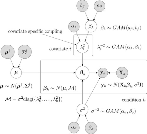4) ). A graphical model representation of the coupled Bayesian regression model is provided in Figure 1.

Figure 1. Graphical model representation of the new hierarchically coupled Bayesian regression model. The mathematical details can be found in Section 3.1. Free (hyper-)parameters are in white circles. The data and fix hyperparameters are in gray circles. The two boxes indicate the experimental conditions $h=1,\dots ,H$ and the covariate-specific coupling parameters $i=0,\dots ,k$.

3.2. Gibbs sampling for given covariates

If the relevant covariates are known (say: $X_1,\dots ,X_k$ like in Section 3.1), they do not have to be inferred from the data. A Gibbs sampling scheme can then be used to generate a posterior sample of the model parameters $\{\{{\mathit{\beta }}_h\},{\sigma }^2,\mathit{\mu },\mathbf{\Sigma },{\beta }_{\lambda }\}$. In the supplementary material we derive the required full conditional distributions, from which the model parameters can be successively re-sampled. One Gibbs sampling iteration consists of the following five consecutive sampling steps:

(G.1)	Sample: $\begin{array}{rl}& {\sigma }^{-2}|(\mathit{\mu },\mathbf{\Sigma },\{{\mathbf{y}}_h\})\\ & \sim \mathrm{GAM}({\alpha }_{\sigma }+\frac{\sum _{h=1}^H{n}_h}{2},{\beta }_{\sigma }+\frac{1}{2}\sum _{h=1}^H({\mathbf{y}}_h-{\mathbf{X}}_h\mathit{\mu }{)}^{\mathsf{T}}(\mathbf{I}+{\mathbf{X}}_h\mathbf{\Sigma }{\mathbf{X}}_h^{\mathsf{T}}{)}^{-1}({\mathbf{y}}_h-{\mathbf{X}}_h\mathit{\mu }))\end{array}$
(G.2)	For $h=1,\dots ,H$ sample: ${\mathit{\beta }}_h|(\mathit{\mu },\mathbf{\Sigma },\{{\mathbf{y}}_h\})\sim \mathcal{N}([{\mathbf{\Sigma }}^{-1}+{\mathbf{X}}_h^{\mathsf{T}}{\mathbf{X}}_h{]}^{-1}({\mathbf{\Sigma }}^{-1}\mathit{\mu }+{\mathbf{X}}_h^{\mathsf{T}}{\mathbf{y}}_h),{\sigma }^2[{\mathbf{\Sigma }}^{-1}+{\mathbf{X}}_h^{\mathsf{T}}{\mathbf{X}}_h{]}^{-1})$
(G.3)	For $i=0,\dots ,k$ sample: ${\lambda }_i^{-2}|(\{{\beta }_{h,i}\},{\sigma }^2,{\mu }_i,{\beta }_{\lambda })\sim \text{GAM}({\alpha }_{\lambda }+\frac{H}{2},{\beta }_{\lambda }+\frac{1}{2}{\sigma }^{-2}\sum _{h=1}^H({\beta }_{h,i}-{\mu }_i{)}^2)$
(G.4)	Sample: ${\beta }_{\lambda }|\mathbf{\Sigma }\sim \text{GAM}(a_{\beta }+(k+1){\alpha }_{\lambda },b_{\beta }+\sum _{i=0}^k{\lambda }_i^{-2})$
(G.5)	Sample: $\mathit{\mu }|({\sigma }^2,\mathbf{\Sigma },\{{\mathbf{y}}_h\})\sim \mathcal{N}({\mathit{\mu }}^{‡},{\mathbf{\Sigma }}^{‡})$ where $\begin{array}{rl}{\mathbf{\Sigma }}^{‡}& ={(\sum _{h=1}^H\left({\mathbf{X}}_h^T{({\sigma }^2[\mathbf{I}+{\mathbf{X}}_h\mathbf{\Sigma }{\mathbf{X}}_h^{\mathsf{T}}])}^{-1}{\mathbf{X}}_h\right)+\{{\mathbf{\Sigma }}^{†}{\}}^{-1})}^{-1}\\ {\mathit{\mu }}^{‡}& ={\mathbf{\Sigma }}^{‡}(\sum _{h=1}^H{\mathbf{X}}_h^T{({\sigma }^2[\mathbf{I}+{\mathbf{X}}_h\mathbf{\Sigma }{\mathbf{X}}_h^{\mathsf{T}}])}^{-1}{\mathbf{y}}_h+\{{\mathbf{\Sigma }}^{†}{\}}^{-1}{\mathit{\mu }}^{†})\end{array}$

We also show in the supplementary material that ${\mathit{\beta }}_h$ ($h=1,\dots ,H$) and ${\sigma }^2$ can be integrated out from the likelihood, $p(\{{\mathbf{y}}_h\}|\{{\mathit{\beta }}_h\},{\sigma }^2)$, yielding the marginal likelihood: (7) $\begin{array}{rl}p(\{{\mathbf{y}}_h\}|\mathit{\mu },\mathbf{\Sigma })& =\frac{\mathrm{\Gamma }(\frac{T}{2}+{\alpha }_{\sigma })}{\mathrm{\Gamma }({\alpha }_{\sigma })}\cdot \frac{{\pi }^{-\frac{T}{2}}(2{\beta }_{\sigma }{)}^{{\alpha }_{\sigma }}}{{(\prod _{h=1}^{H}det({\mathbf{C}}_h))}^{1/2}}\\ & \cdot {(2{\beta }_{\sigma }+\sum _{h=1}^H({\mathbf{y}}_h-{\mathbf{X}}_h\mathit{\mu }{)}^{\mathsf{T}}{\mathbf{C}}_h^{-1}({\mathbf{y}}_h-{\mathbf{X}}_h\mathit{\mu }))}^{-(\frac{T}{2}+{\alpha }_{\sigma })}\end{array}$(7) where ${\mathbf{C}}_h:=\mathbf{I}+{\mathbf{X}}_h\mathbf{\Sigma }{\mathbf{X}}_h^{\mathsf{T}}$ and $T:=\sum _{h=1}^H{n}_h$ is the total number of observations. In terms of the marginal likelihood, we have for the posterior density: (8) $p(\mathit{\mu },\mathbf{\Sigma },{\beta }_{\lambda }|\{{\mathbf{y}}_h\})\propto p(\{{\mathbf{y}}_h\}|\mathit{\mu },\mathbf{\Sigma })\cdot p(\mathit{\mu })\cdot p(\mathbf{\Sigma }|{\beta }_{\lambda })\cdot p({\beta }_{\lambda })$(8) where $\mathbf{\Sigma }=\text{diag}(\{{\lambda }_0^2,\dots ,{\lambda }_k^2\})$ is the diagonal matrix of the coupling parameters.

We note that the RJMCMC moves between covariate sets, which we describe in Section 3.3, make use of the marginal likelihood from Equation (7(7) $\begin{array}{rl}p(\{{\mathbf{y}}_h\}|\mathit{\mu },\mathbf{\Sigma })& =\frac{\mathrm{\Gamma }(\frac{T}{2}+{\alpha }_{\sigma })}{\mathrm{\Gamma }({\alpha }_{\sigma })}\cdot \frac{{\pi }^{-\frac{T}{2}}(2{\beta }_{\sigma }{)}^{{\alpha }_{\sigma }}}{{(\prod _{h=1}^{H}det({\mathbf{C}}_h))}^{1/2}}\\ & \cdot {(2{\beta }_{\sigma }+\sum _{h=1}^H({\mathbf{y}}_h-{\mathbf{X}}_h\mathit{\mu }{)}^{\mathsf{T}}{\mathbf{C}}_h^{-1}({\mathbf{y}}_h-{\mathbf{X}}_h\mathit{\mu }))}^{-(\frac{T}{2}+{\alpha }_{\sigma })}\end{array}$(7) ) and the relationship given in Equation (8(8) $p(\mathit{\mu },\mathbf{\Sigma },{\beta }_{\lambda }|\{{\mathbf{y}}_h\})\propto p(\{{\mathbf{y}}_h\}|\mathit{\mu },\mathbf{\Sigma })\cdot p(\mathit{\mu })\cdot p(\mathbf{\Sigma }|{\beta }_{\lambda })\cdot p({\beta }_{\lambda })$(8) ).

3.3. Metropolis-Hastings sampling of the covariates

In many applications the true covariates are not known and have to be inferred from the data. We assume that there are n potential covariates $X_1,\dots ,X_n$, and we let $\mathit{\pi }\subset \{X_1,\dots ,X_n\}$ denote a subset of covariates with prior probability $p(\mathit{\pi })$. Moreover, we write $p(\{{\mathbf{y}}_h\}|\mathit{\mu },\mathbf{\Sigma },\mathit{\pi })$ to denote the marginal likelihood implied by the covariate set $\mathit{\pi }$, where we do not make explicit that $\mathit{\mu }$ and $\mathbf{\Sigma }$ depend on $\mathit{\pi }$. For generating a posterior sample of covariate sets we employ the marginal likelihood from Equation (7(7) $\begin{array}{rl}p(\{{\mathbf{y}}_h\}|\mathit{\mu },\mathbf{\Sigma })& =\frac{\mathrm{\Gamma }(\frac{T}{2}+{\alpha }_{\sigma })}{\mathrm{\Gamma }({\alpha }_{\sigma })}\cdot \frac{{\pi }^{-\frac{T}{2}}(2{\beta }_{\sigma }{)}^{{\alpha }_{\sigma }}}{{(\prod _{h=1}^{H}det({\mathbf{C}}_h))}^{1/2}}\\ & \cdot {(2{\beta }_{\sigma }+\sum _{h=1}^H({\mathbf{y}}_h-{\mathbf{X}}_h\mathit{\mu }{)}^{\mathsf{T}}{\mathbf{C}}_h^{-1}({\mathbf{y}}_h-{\mathbf{X}}_h\mathit{\mu }))}^{-(\frac{T}{2}+{\alpha }_{\sigma })}\end{array}$(7) ) and we implement three RJMCMC moves:

(D)	In the deletion move we randomly choose a covariate $X_j\in \mathit{\pi }$, and we propose to remove $X_j$ from the covariate set $\mathit{\pi }$.
(A)	In the addition move we randomly select one covariate $X_i\notin \mathit{\pi }$, and we propose to add $X_i$ to the covariate set $\mathit{\pi }$.
(E)	In the exchange move we randomly select one covariate $X_j\in \mathit{\pi }$, and we propose to replace $X_j$ by a randomly selected new covariate $X_i\notin \mathit{\pi }$.

Each move yields a new covariate set ${\mathit{\pi }}^{\star }$, and we propose to replace the current $\mathit{\pi }$ by ${\mathit{\pi }}^{\star }$. Since the global mean vector $\mathit{\mu }$ and the diagonal matrix of variance multipliers $\mathbf{\Sigma }$ refer to the original covariate set $\mathit{\pi }$, we have to adjust them for ${\mathit{\pi }}^{\star }$. Therefore, along with the new covariate set ${\mathit{\pi }}^{\star }$ we also have to propose a new vector ${\mathit{\mu }}^{\star }$ and a new matrix ${\mathbf{\Sigma }}^{\star }$.

• The addition and the exchange move both add a new covariate $X_i$ to π. For this new covariate we sample the variance multiplier ${\lambda }_i^{2,\star }$ from its prior distribution, $p({\lambda }_i^{2,\star }|{\beta }_{\lambda })$, and we add the new element to $\mathbf{\Sigma }$. The deletion move and the exchange move both remove one covariate $X_j$ from $\mathit{\pi }$ and we also remove the corresponding multiplier ${\lambda }_j^2$ from $\mathbf{\Sigma }$. Let ${\mathbf{\Sigma }}^{\star }$ denote the resulting new variance multiplier matrix.³

• Given ${\mathit{\pi }}^{\star }$ and ${\mathbf{\Sigma }}^{\star }$, we also sample a new global mean vector ${\mathit{\mu }}^{\star }$ from its full conditional distribution, $p({\mathit{\mu }}^{\star }|\{{\mathbf{y}}_h\},{\sigma }^2,{\mathbf{\Sigma }}^{\star },{\mathit{\pi }}^{\star })$; cf. step (G.5) of Section 3.2.

When randomly selecting the move type, the acceptance probability for the move from $[\mathit{\pi },\mathbf{\Sigma },\mathit{\mu }]$ to $[{\mathit{\pi }}^{\star },{\mathbf{\Sigma }}^{\star },{\mathit{\mu }}^{\star }]$ is: $A([\mathit{\pi },\mathbf{\Sigma },\mathit{\mu }],[{\mathit{\pi }}^{\star },{\mathbf{\Sigma }}^{\star },{\mathit{\mu }}^{\star }])=min\{1,\frac{p(\{{\mathbf{y}}_h\}|{\mathit{\mu }}^{\star },{\mathbf{\Sigma }}^{\star },{\mathit{\pi }}^{\star })}{p(\{{\mathbf{y}}_h\}|\mathit{\mu },\mathbf{\Sigma },\mathit{\pi })}\cdot \frac{p({\mathit{\mu }}^{\star })}{p(\mathit{\mu })}\cdot \frac{p({\mathbf{\Sigma }}^{\star })}{p(\mathbf{\Sigma })}\cdot \frac{p({\mathit{\pi }}^{\star })}{p(\mathit{\pi })}\cdot \text{HR}\}$ with the Hastings inverse proposal ratio (HR) $\text{HR}=\frac{p(\mathbf{\Sigma })}{p({\mathbf{\Sigma }}^{\star })}\cdot \frac{p(\mathit{\mu }|\{{\mathbf{y}}_h\},{\sigma }^2,\mathbf{\Sigma },\mathit{\pi })}{p({\mathit{\mu }}^{\star }|\{{\mathbf{y}}_h\},{\sigma }^2,{\mathbf{\Sigma }}^{\star },{\mathit{\pi }}^{\star })}\cdot \{\begin{array}{ll}{\displaystyle \frac{|\pi |}{n-|{\pi }^{\star }|}}& \text{for (D)}\\ {\displaystyle \frac{n-|\pi |}{|{\pi }^{\star }|}}& \text{for (A)}\\ 1& \text{for (E)}\end{array}$ where n is the number of potential covariates, and $|\cdot |$ denotes the cardinality.⁴

3.4. Model inference

For model inference we combine the Gibbs sampling moves from Section 3.2 with the RJMCMC moves from Section 3.3, so as to generate a posterior sample: ${\{\{{\mathit{\beta }}_h^{[r]}\},{\sigma }_{[r]}^2,{\mathit{\mu }}^{[r]},{\mathbf{\Sigma }}^{[r]},{\beta }_{\lambda }^{[r]},{\mathit{\pi }}^{[r]}\}}_{r=1,\dots ,R}$ where we do not make explicit that each ${\mathit{\beta }}_h^{[r]}$, ${\mathit{\mu }}^{[r]}$ and ${\mathbf{\Sigma }}^{[r]}$ depend on the covariate set ${\mathit{\pi }}^{[r]}$. From the RJMCMC sample we can estimate for each of the n covariates a marginal inclusion probability. For example, for covariate $X_i$ we get: (9) $\hat{p}(X_i\in \mathit{\pi }|\{{\mathbf{y}}_h\})=\frac{1}{R}\sum _{r=1}^R{\mathcal{I}}_{{\mathit{\pi }}^{[r]}}(X_i)$(9) where ${\mathcal{I}}_{{\mathit{\pi }}^{[r]}}(X_i)=1$ if $X_i\in {\mathit{\pi }}^{[r]}$, and ${\mathcal{I}}_{{\mathit{\pi }}^{[r]}}(X_i)=0$ otherwise. That is, the estimator is the relative frequency of sampled covariate sets that obtained covariate $X_i$.

Moreover, we can estimate the predictive probability of a new target vector ${\tilde{\mathbf{y}}}_h$ taken under condition h. Let ${\tilde{\mathbf{X}}}_{h,\mathit{\pi }}$ denote the corresponding design matrix built from the covariates of the set $\mathit{\pi }$. The estimated predictive probability is: (10) $\hat{p}({\tilde{\mathbf{y}}}_h|\{{\mathbf{y}}_h\})=\frac{1}{R}\sum _{r=1}^{R}p({\tilde{\mathbf{y}}}_h|{\mathit{\beta }}_h^{[r]},{\sigma }_{[r]}^2,{\mathit{\pi }}^{[r]})$(10) where $p(.|{\mathit{\beta }}_h^{[r]},{\sigma }_{[r]}^2,{\mathit{\pi }}^{[r]})$ is the density of the $\mathcal{N}({\tilde{\mathbf{X}}}_{h,{\mathit{\pi }}^{[r]}}\cdot {\mathit{\beta }}_h^{[r]},{\sigma }_{[r]}^2\mathbf{I})$ distribution.

3.5. From Bayesian regression to dynamic Bayesian networks

Consider $N$ variables $Z_1,\dots ,Z_N$ that were observed under conditions $h=1,\dots ,H$. Let $z_{i,t,h}$ be the observation of $Z_i$ under condition h at time point $t\in \{1,\dots ,{\tilde{n}}_h\}$, where ${\tilde{n}}_h:=n_h+1$. The goal is to infer the interactions among the variables, where all interactions are subject to a lag of one time point. That is, each interaction $Z_i\to Z_j$ indicates that $z_{i,t,h}$ has an effect on $z_{j,t+1,h}$ ($h=1,\dots ,H$ and $t=1,\dots ,n_h$). Because of the time lag, the network model can be separated into N independent regression models, whose effective sample sizes reduce from ${\tilde{n}}_h$ to $n_h={\tilde{n}}_h-1$.

In the wth regression model $Z_w$ takes the role of the target variable, Y, and the remaining $(N-1)=:n$ variables $Z_q$ ($q\ne w$) are the potential covariates $X_1,\dots ,X_n$. Because of the data structure, the hierarchically coupled Bayesian regression model from Section 3.1 can be employed and covariate sets ${\mathit{\pi }}_w$ for $Z_w$ can be MCMC sampled, as described in Section 3.4. The condition-specific response vectors are given by ${\mathbf{y}}_h^w=(z_{w,2,h},\dots ,z_{w,n_h+1,h}{)}^{\mathsf{T}}\in {\mathbb{R}}^{n_h}(h=1,\dots ,H)$ while the corresponding design matrices ${\mathbf{X}}_h^w$ contain the values of the covariates from ${\mathit{\pi }}_w$. When $Z_q\in {\mathit{\pi }}_w$, design matrix ${\mathbf{X}}_h^w$ contains the column $(z_{q,1,h},\dots ,z_{q,n_h,h}{)}^{\mathsf{T}}$. For each variable $Z_w$ a regression model posterior sample can be generated: ${\{\{{\mathit{\beta }}_h^{w,[r]}\},{\sigma }_{w,[r]}^2,{\mathit{\mu }}_w^{[r]},{\mathbf{\Sigma }}_w^{[r]},{\beta }_{\lambda }^{w,[r]},{\mathit{\pi }}_w^{[r]}\}}_{r=1,\dots ,R}(w=1,\dots ,N)$ The variable-specific covariate sets that were sampled in iteration r, symbolically ${\mathit{\pi }}_1^{[r]},\dots ,{\mathit{\pi }}_N^{[r]}$, can then be merged to a network ${\mathbf{N}}^{[r]}:=\{{\mathit{\pi }}_1^{[r]},\dots ,{\mathit{\pi }}_N^{[r]}\}$. The rth network ${\mathbf{N}}^{[r]}$ features the regulatory interaction $Z_i\to Z_j$ if $Z_i\in {\mathit{\pi }}_j^{[r]}$. Henceforth, the marginal covariate inclusion probabilities from Equation (9(9) $\hat{p}(X_i\in \mathit{\pi }|\{{\mathbf{y}}_h\})=\frac{1}{R}\sum _{r=1}^R{\mathcal{I}}_{{\mathit{\pi }}^{[r]}}(X_i)$(9) ) can then be interpreted as marginal network interaction probabilities.

Given additional new data points that were measured under condition h and that yield the N variable-specific response vectors ${\tilde{\mathbf{y}}}_h^1,\dots ,{\tilde{\mathbf{y}}}_h^N$ the predictive probability from Equation (10(10) $\hat{p}({\tilde{\mathbf{y}}}_h|\{{\mathbf{y}}_h\})=\frac{1}{R}\sum _{r=1}^{R}p({\tilde{\mathbf{y}}}_h|{\mathit{\beta }}_h^{[r]},{\sigma }_{[r]}^2,{\mathit{\pi }}^{[r]})$(10) ) extends to (11) $\hat{p}({\tilde{\mathbf{y}}}_h^1,\dots ,{\tilde{\mathbf{y}}}_h^N|\{{\mathbf{y}}_h^1,\dots ,{\mathbf{y}}_h^N\})=\frac{1}{R}\sum _{r=1}^R(\prod _{w=1}^{N}p({\tilde{\mathbf{y}}}_h^w|{\mathit{\beta }}_h^{w,[r]},{\sigma }_{w,[r]}^2,{\mathit{\pi }}_w^{[r]}))$(11) where $p(.|{\mathit{\beta }}_h^{w,[r]},{\sigma }_{w,[r]}^2,{\mathit{\pi }}_w^{[r]})$ is the density of the $\mathcal{N}({\tilde{\mathbf{X}}}_{h,{\mathit{\pi }}_w^{[r]}}^w\cdot {\mathit{\beta }}_h^{w,[r]},{\sigma }_{w,[r]}^2\mathbf{I})$ distribution.

3.6. Leave-one-out-cross-validation

For objectively comparing the performances of different methods, we propose to apply a leave-one-out-cross-validation (LOOCV) approach and to Monte Carlo approximate the predictive probabilities (PPS) for the left out data points using Equation (11(11) $\hat{p}({\tilde{\mathbf{y}}}_h^1,\dots ,{\tilde{\mathbf{y}}}_h^N|\{{\mathbf{y}}_h^1,\dots ,{\mathbf{y}}_h^N\})=\frac{1}{R}\sum _{r=1}^R(\prod _{w=1}^{N}p({\tilde{\mathbf{y}}}_h^w|{\mathit{\beta }}_h^{w,[r]},{\sigma }_{w,[r]}^2,{\mathit{\pi }}_w^{[r]}))$(11) ).

To this end, we loop through the conditions $h=1,\dots ,H$, and within each condition h we loop through the time points $t=2,\dots ,n_h+1$. For each $(h,t)$ we then remove for each variable $Z_w$ ($w\in \{1,\dots ,N\}$) the value $z_{w,t,h}$ from response vector ${\mathbf{y}}_h^w$ and run a regression MCMC simulation using the reduced response vector ${\mathbf{y}}_h^w\mathrm{\setminus }{z}_{w,t,h}$. Performing a regression MCMC simulation on each reduced response vector ${\mathbf{y}}_h^w\mathrm{\setminus }{z}_{w,t,h}$ ($w=1,\dots ,N$) yields N MCMC outputs, which we can use to estimate the predictive probability for the new (left-out) observation $({\tilde{\mathbf{y}}}_h^1,\dots ,{\tilde{\mathbf{y}}}_h^N):=(z_{1,t,h},\dots ,z_{N,t,h})$ using Equation (11(11) $\hat{p}({\tilde{\mathbf{y}}}_h^1,\dots ,{\tilde{\mathbf{y}}}_h^N|\{{\mathbf{y}}_h^1,\dots ,{\mathbf{y}}_h^N\})=\frac{1}{R}\sum _{r=1}^R(\prod _{w=1}^{N}p({\tilde{\mathbf{y}}}_h^w|{\mathit{\beta }}_h^{w,[r]},{\sigma }_{w,[r]}^2,{\mathit{\pi }}_w^{[r]}))$(11) ). In total, we get the predictive probabilities for $T=\sum _{h=1}^H{n}_h$ network data points (cf. Section 3.5), by generating posterior samples for $N\cdot T$ hierarchical Bayesian regression models (cf. Sections 3.1–3.4).

3.7. Data imputation methods to predict equidistant covariate values

The immunoblotting mTOR protein data have been measured under two conditions ($h=1,2)$ at ${\tilde{n}}_h=10$ non-equidistant time points, $t^{\diamond }\in \{0,1,3,5,10,15,30,45,60,120\}$, cf. Section 2. That is, for each phosphorylation site $Z_w$ ($w=1,\dots ,11$) we only have the observations $z_{w,t^{\diamond },h}$ (h = 1, 2 and $t^{\diamond }\in \{0,1,3,\dots ,45,60,120\}$) rather than equidistant observations. The experimental design has been in mismatch to one of the key assumptions of dynamic Bayesian networks, namely the assumption that the made observations are equidistant. This mismatch between data and model is typically ignored and the naive simple shift (SH) approach is to treat the data as if they were equidistant. With regard to our mTOR application, the SH approach implies combining measurements that refer to protein phosphorylation processes that took place in substantially different time intervals, ranging from 1 to 60 min.

In this paper we show that the naive SH approach yields inaccurate results, and we propose an alternative approach to deal with non-equidistant network measurements. We consider the observed non-equidistant time series as incomplete, and we propose to make use of established data imputation techniques to predict the required unobserved equidistant preceding covariate values. For example, the last nine non-equidistant observations of site $Z_w$ under condition h become the elements of the response vectors: ${\mathbf{y}}_h^w:=(z_{w,1,h},z_{w,3,h},z_{w,5,h},\dots ,z_{w,45,h},z_{w,60,h},z_{w,120,h}{)}^{\mathsf{T}}\in {\mathbb{R}}^{n_h=9}(h=1,2)$ When $Z_q$ ($q\ne w$) is a covariate, we do not follow the naive SH approach and fill the corresponding column of the design matrix ${\mathbf{X}}_h^w$ with the nine observations at the non-equidistant preceding points $\{z_{q,t^{\diamond },h}:t^{\diamond }\in \{0,1,3,5,10,15,30,45,60\}\}$ but we fill the design matrix ${\mathbf{X}}_h^w$ with nine predicted equidistant observations $\{{\hat{z}}_{q,t^{\diamond }-1,h}:t^{\diamond }\in \{1,3,5,10,15,30,45,60,120\}\}$ so that each (predicted) covariate value ${\hat{z}}_{q,t^{\diamond }-1,h}$ is exactly one minute before the corresponding (observed) response value $z_{w,t^{\diamond },h}$. We note that the initial covariate values at time point t = 0 have actually been observed and do not need to be estimated by the data imputation methods. That is, instead of estimating ${\hat{z}}_{q,t^{\diamond }-1,h}$ for $t^{\diamond }=1$, we can use the actually observed covariate value $z_{q,0,h}$. This only applies to $t^{\diamond }=1$, since the first two measurements are subject to a time lag of exactly one minute.

In our study, we compare the naive simple shift approach (SH) with various data imputation techniques, such as a simple linear interpolation (LI), three moving average approaches (SM, LW, EW), smoothing splines (SP), Gaussian processes (GP), Kalman smoothing (KS), and local polynomial regression fitting (LO). For an overview of the 8 data imputation methods we refer to Table 2. For all imputation methods we used the default settings of the employed R software packages without trying to optimize their performances. For example, we only applied Gaussian processes with the squared exponential kernel. Moreover, we note that we initialized the Kalman smoothing method with the truly observed covariate values at time point $t^{\diamond }=0$.

Table 2. Overview of the 8 data imputation methods that we considered in our study.

Abbrev.	Interpolation method	Reference and implementation
LI	linear interpolation	R package ‘imputeTS’
		see [9] for the detail of the package
KS	Kalman smoothing	See, e.g. [4,15].
		R package ‘imputeTS’
EW	exponential-weighted moving average	See, e.g. [1,6].
		R package ‘imputeTS’
LW	linear-weighted moving average	R package ‘imputeTS’.
SM	simple moving average	R package ‘imputeTS’.
GP	Gaussian process	R package ‘GauPro’.
		see [3] for the detail of the package
SP	smoothing splines	R package ‘stats’.
		under the function ‘smooth.spline’
LO	local polynomial regression fitting	R package ‘stats’.
		under the function ‘loess’

Notes: Instead of treating non-equidistant data as if they were equidistant (naive simple shift (SH) approach), we propose to use data imputation methods to predict the missing equidistant observations.

4. Competing methods and implementation details

4.1. Competing network models

We compare the performance of the proposed new NH-DBN model from Section 3 with three competing NH-DBN models. The competing models are conceptually similar but base on alternative regression approaches (cf. Section 3.1).

• A conventional DBN merges the data from all conditions $\mathbf{y}:=({\mathbf{y}}_1^{\mathsf{T}},\dots ,{\mathbf{y}}_H^{\mathsf{T}}{)}^{\mathsf{T}}$ and assumes the same regression coefficient vector $\mathit{\beta }\in {\mathbb{R}}^{k+1}$ for all data points. In replacement of Equations (1(1) ${\mathbf{y}}_h|({\mathit{\beta }}_h,{\sigma }^2)\sim \mathcal{N}({\mathbf{X}}_h{\mathit{\beta }}_h,{\sigma }^2\mathbf{I})(h=1,\dots ,H)$(1) )–(2(2) $\begin{array}{rl}{\mathit{\beta }}_h|(\mathit{\mu },{\sigma }^2,\mathbf{\Sigma })& \sim \mathcal{N}(\mathit{\mu },\mathcal{M})(h=1,\dots ,H)\\ \mathit{\mu }& \sim \mathcal{N}({\mathit{\mu }}^{†},{\mathbf{\Sigma }}^{†})\end{array}$(2) ) we get $\mathbf{y}|(\mathit{\beta },{\sigma }^2)\sim \mathcal{N}(\mathbf{X}\mathit{\beta },{\sigma }^2\mathbf{I})$ where $\mathbf{X}:=({\mathbf{X}}_1^{\mathsf{T}},\dots ,{\mathbf{X}}_H^{\mathsf{T}}{)}^{\mathsf{T}}$, $\mathit{\beta }|({\sigma }^2,{\lambda }^2)\sim \mathcal{N}(\mathbf{0},{\sigma }^2{\lambda }^2\mathbf{I})$, and ${\lambda }^{-2}\sim \text{GAM}({\alpha }_{\lambda },{\beta }_{\lambda })$.

• An uncoupled non-homogeneous DBN (‘UC’) assumes the regression coefficient vectors to be condition-specific but it does not encourage the vectors to stay similar across conditions. The prior from Equation (2(2) $\begin{array}{rl}{\mathit{\beta }}_h|(\mathit{\mu },{\sigma }^2,\mathbf{\Sigma })& \sim \mathcal{N}(\mathit{\mu },\mathcal{M})(h=1,\dots ,H)\\ \mathit{\mu }& \sim \mathcal{N}({\mathit{\mu }}^{†},{\mathbf{\Sigma }}^{†})\end{array}$(2) ) becomes ${\mathit{\beta }}_h|({\sigma }^2,{\lambda }^2)\sim \mathcal{N}(\mathbf{0},{\sigma }^2{\lambda }^2\mathbf{I})(h=1,\dots ,H)$ where ${\lambda }^{-2}\sim \text{GAM}({\alpha }_{\lambda },{\beta }_{\lambda })$.

• The globally coupled non-homogeneous DBN (‘GLOBAL’) is similar to the proposed model but less flexible, as it uses the same coupling parameter ${\lambda }^2$ for all covariates [7,8]. Hence, it enforces the same coupling strength for all covariates, and the prior from Equation (2(2) $\begin{array}{rl}{\mathit{\beta }}_h|(\mathit{\mu },{\sigma }^2,\mathbf{\Sigma })& \sim \mathcal{N}(\mathit{\mu },\mathcal{M})(h=1,\dots ,H)\\ \mathit{\mu }& \sim \mathcal{N}({\mathit{\mu }}^{†},{\mathbf{\Sigma }}^{†})\end{array}$(2) ) becomes ${\mathit{\beta }}_h|({\sigma }^2,{\lambda }^2)\sim \mathcal{N}(\mathit{\mu },{\sigma }^2{\lambda }^2\mathbf{I})(h=1,\dots ,H)$ where ${\lambda }^{-2}\sim \text{GAM}({\alpha }_{\lambda },{\beta }_{\lambda })$ is a shared coupling parameter for all k + 1 covariates.

4.2. Hyperparameter settings and simulation details

The (hyper-)parameter setting for which we obtained the results reported in Section 5 can be found in Table 3. Since our new model is an improved version of the globally coupled NH-DBN model from [7,8], which we referred to as ‘GLOBAL’ in Section 4.1, we decided to stay close to the earlier studies and to re-employ the same prior hyperparameters that were already used in the earlier studies; cf. the hyperparameter setting listed in Table 3.

Table 3. List of the (hyper-)prior distributions along with the selected fix hyperparameters.

(Hyper-)parameter	(Hyper-)prior	Fix (hyper-)parameters
${\mathit{\beta }}_h$	$\mathcal{N}(\mathit{\mu },\mathcal{M}$ )	$\mathit{\mu }$ is free
		$\mathcal{M}={\sigma }^2\mathbf{\Sigma }$
		where $\mathbf{\Sigma }=\text{diag}(\{{\lambda }_0^2,\dots ,{\lambda }_k^2\})$
$\mathit{\mu }$	$\mathcal{N}({\mathit{\mu }}^{†},{\mathbf{\Sigma }}^{†})$	${\mathit{\mu }}^{†}=\mathbf{0}$ and ${\mathbf{\Sigma }}^{†}=\mathbf{I}$
${\sigma }^{-2}$	$\mathrm{GAM}({\alpha }_{\sigma },{\beta }_{\sigma })$	${\alpha }_{\sigma }=0.005$ and ${\beta }_{\sigma }=0.005$
${\lambda }_i^{-2}$	$\mathrm{GAM}({\alpha }_{\lambda },{\beta }_{\lambda })$	${\alpha }_{\lambda }=2$ and ${\beta }_{\lambda }$ is free
${\beta }_{\lambda }$	$\mathrm{GAM}(a_{\beta },b_{\beta })$	$a_{\beta }=0.2$ and $b_{\beta }=1$

For the mTOR data we also performed additional RJMCMC simulations with different (hyper-)parameter settings to test for model robustness. In consistency with the findings of the sensitivity study reported in [7], the alternative hyperparameter settings led to comparable results in terms of the marginal network interaction probabilities. Table 3 of the supplementary material lists the alternative hyperparameter settings and Figure 2 of the supplementary material shows scatter plots of the resulting marginal network interaction probabilities. From the individual scatter plots it can be seen that the hyperparameter settings yield very similar marginal network interaction probabilities, indicating that the newly proposed model is robust with respect to the (hyper-)parameters of the prior distributions.

We run all RJMCMC simulations for 100,000 iterations and we withdraw the samples generated during the first $\mathrm{50,000}$ iterations to take a burn-in phase into account. To check for RJMCMC convergence we ran various independent RJMCMC simulations with different random seeds on the mTOR data set. Scatter plots of the marginal network interaction probabilities suggest sufficient convergence after 100,000 RJMCMC iterations. A few example scatter plots are shown in Figure 1 of the supplementary material. From the scatter plots it can be seen that independent and differently seeded RJMCMC simulations lead to (approximately) the same marginal network interaction probabilities. Since we obtain a concrete predicted network by imposing a threshold on those interaction probabilities and showing only those interactions whose probabilities exceed the threshold, we conclude that independent RJMCMC simulations yield exactly the same predicted mTOR pathway; see Figure 5.

5. Results

To identify the best combination of data imputation method and NH-DBN model, we perform a systematic comparative evaluation study; cf. Section 5.1. We then employ the best combination to statistically learn the structure of the mTOR protein signaling pathway; cf. Section 5.2.

5.1. Comparative evaluation study

In our comparative evaluation study, we follow a LOOCV approach and we compute predictive probabilities (PPs) for the left-out data points. For the mathematical details we refer to Section 3.6. The goal of our study is to cross-compare the performances of the four NH-DBN models (cf. Figure 1 and the three competitors from Section 4.1) and the data imputation methods (cf. Table 2). For every combination of NH-DBN model and data imputation method we can compute 18 predictive probabilities (PPs), and we refer to them as the LOOCV-PPs. For each of model-method combination Figure 2 shows a boxplot of the LOOCV-PP value distributions. The black reference lines indicate the median of the combination newly proposed NH-DBN (NEW) with smoothing splines based data imputation (SP). The first obvious finding is that the globally coupled model (GLOBAL) and the newly proposed model (NEW) perform clearly better than the homogeneous DBN and the uncoupled NH-DBN (UC). Furthermore, it can be easily seen from Figure 2 that the data imputation methods also have clear effects on the LOOCV-PP distributions. In Sections 5.1.1 and 5.1.2 we therefore have a closer look at the 9 data imputation methods and at the 4 NH-DBN models, respectively.

Figure 2. Raw data: Boxplots of the logarithmic predictive probabilities (PPs), obtained by leave-one-out-cross validation (LOOCV-PPs). For each of the four NH-DBN models (DBN, UC, GLOBAL and NEW) there is a separate panel. And within each panel there are 9 boxplots that refer to the 9 data interpolation methods for missing data (see Table 2). Each of the 36 boxplots displays the distribution of 18 predictive probabilities (one for each left-out data point). The black horizontal lines mark the largest boxplot median, which was achieved by the new NH-DBN model (NEW) in combination with smoothing splines (SP). Relevant pairwise comparisons of the log LOOCV-PPs can be found in Figures 3 and 4.

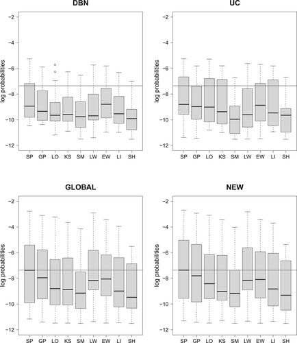
Figure 3. Comparing the data imputation methods; cf. Table 2. Boxplots of the absolute LOOCV-PP values have been provided in Figure 2. The 32 boxplots of this figure refer to the relative LOOCV-PP differences in favor of the smoothing splines interpolation method (SP). For each of the four NH-DBN models (DBN, UC, GLOBAL and NEW) there is a separate panel. Within each panel there are 8 boxplots showing the pairwise differences in the logarithmic predictive probabilities in favor of the smoothing splines (SP). The black horizontal lines mark the zero line. For the data imputation methods behind the abbreviations we refer to Table 2. It can be seen that all differences are consistently in favor of the smoothing splines (SP).

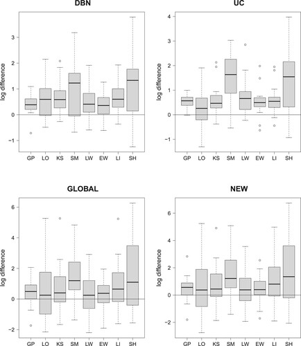
Figure 4. Comparing the four NH-DBN models. Boxplots of the absolute LOOCV-PP values were provided in Figure 2. The 27 boxplots of this figure refer to the pairwise relative LOOCV-PP differences in favor of the newly proposed NH-DBN (NEW). There are 9 panels, one for each data interpolation method. Within each panel there are three boxplots showing the relative differences in the logarithmic predictive probabilities in favor of the newly proposed NH-DBN model (NEW). Left boxplot: NEW vs. DBN, center boxplot: NEW vs. UC and right boxplot: NEW vs. GLOBAL. In each panel a black horizontal line marks the zero line. It can be seen that all differences are consistently in favor of the newly proposed NH-DBN (NEW).

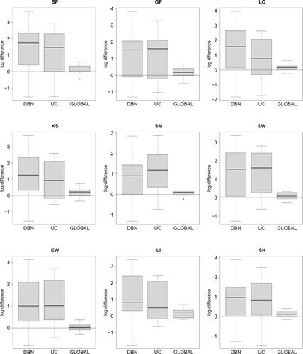
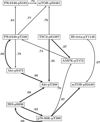
Figure 5. Predicted mTOR protein signaling pathway. Based on the results of our comparative evaluation study in Section 5.1, we employed the newly proposed hierarchical Bayesian model from Section 3.1 (NEW) in combination with smoothing splines (SP) to infer the structure of the mTOR pathway from all data points. By running a RJMCMC for each site $Z_w$ we posterior sampled the site-specific regulator sets (subsets of the n = 10 other sites). The marginal network interaction probability for the interaction $Z_i\to Z_j$ refers to the proportion of posterior sampled covariate sets of site $Z_j$ that contained site $Z_i$ as covariate. Shown are the 16 regulatory interactions whose probabilities exceeded the threshold of 0.7. Interactions whose probabilities exceeded the more conservative threshold of 0.9 are displayed by bold edges.

5.1.1. Comparing the data imputation methods

In each of the four panels of Figure 2 the smoothing splines approaches (SP) led to the largest medians. To inspect whether the differences are statistically significant, Figure 3 shows boxplots of the pairwise differences of the log LOOCV-PP values in favor of the SP method. There are 8 pairwise comparisons per panel (per NH-DBN model); i.e. 32 pairwise comparisons in total. The p-values of two-sided Wilcoxon signed-rank tests are provided in Table 1 of the supplementary material. Although the differences are consistently in favor of the smoothing splines (SP), some of the differences are not statistically significant. The main results can be summarized as follows: Most importantly, the smoothing splines method clearly (and significantly) outperforms the widely applied naive simple shift method (SI) as well as the linear interpolation method (LI), which produces jagged (non-smooth) interpolation curves. Most competitive to the smoothing splines (SP) seem to be the LOESS (LO) method (three p-values greater $\alpha =0.05$) and the linear-weighted moving average (LW) method (two p-values greater than $\alpha =0.05$).

5.1.2. Comparing the NH-DBN models

Figure 4 shows boxplots of the pairwise differences of the log LOOCV-PPs in favor of the newly proposed hierarchically coupled NH-DBN (NEW) from Section 3.1. For all 9 data imputation methods the homogeneous DBN and the uncoupled model (UC) perform much worse than the newly proposed model. Also the globally coupled model (GLOBAL) is outperformed, but here the relative differences are smaller. The p-values of 27 two-sided Wilcoxon signed-rank tests are provided in Table 2 of the supplementary material. The p-values for the comparisons with the models DBN and UC are all smaller than $\alpha =0.05$, but only for 5 out of 9 interpolation methods the newly proposed model performs significantly better than the globally coupled model. For Kalman Smoothing (KS), for exponential- and linear-weighted moving averages (EW and LW), as well as for Gaussian processes (GPs) the differences are not significant, but yet in favor of the newly proposed model (NEW).

5.2. Learning the structure of the mTOR signaling pathway

The results of our comparative evaluation study from Section 5.1 suggest that the smoothing splines data interpolation method along with the newly proposed hierarchically coupled model from Section 3.1 yields the best network learning performance.

We therefore employ this combination for predicting the structure of the mTOR protein signaling pathway from all data points. To this end, we run RJMCMC simulations for each of the N = 11 phosphorylation sites listed in Table 1, so as to infer the site-specific regulators. In the wth RJMCMC simulation phosphorylation site $Z_w$ takes the role of the response and the remaining n = 10 sites become the potential covariates. Via RJMCMC simulation we then sample the covariate subsets (= regulator sets) of site $Z_w$ from the posterior distribution. The marginal covariate inclusion probabilities are the relative frequencies with which the posterior sampled covariate sets for $Z_w$ contained the corresponding covariates; see Equation (9(9) $\hat{p}(X_i\in \mathit{\pi }|\{{\mathbf{y}}_h\})=\frac{1}{R}\sum _{r=1}^R{\mathcal{I}}_{{\mathit{\pi }}^{[r]}}(X_i)$(9) ). By merging all possible inclusion probabilities, we get a probability for each potential network interaction. The marginal network interaction probability for the interaction $Z_i\to Z_j$ is the relative frequency of posterior sampled covariate sets of site $Z_j$ that contained site $Z_i$ as covariate. For a more thorough mathematical description we refer to Section 3.5.

The predicted mTOR pathway is shown in Figure 5. To avoid a very densely connected network, the figure shows only those 16 protein interactions whose marginal probabilities exceeded the threshold of 0.7.

6. Discussion and conclusions

The focus of this paper has been on predicting the structure of the mTOR protein signaling pathway from protein phosphorylation data. We have proposed a hierarchical Bayesian regression model and we used it as building block for a new NH-DBN model. Since data were measured at non-equidistant time points, we have considered established data imputation methods to predict unobserved equidistant data points. Since most of the interactions of the true mTOR network are still unknown, it was not possible to objectively compare the network reconstruction accuracies of different approaches. Therefore, we have proposed a LOOCV strategy to cross-compare the performances in terms of predictive probabilities (PPs). The empirical results of our comparative evaluation study have shown the following trends. First, the smoothing splines method (SP) performed best in predicting the missing data points, while the widely applied and rather naive simple shift approach (SH), which treats non-equidistant data as if they were equidistant, showed consistently the worst performance. Second, we found that the new NH-DBN model performed better than three earlier proposed models. Since the newly proposed NH-DBN model can be seen as a consensus model between the uncoupled and the globally coupled NH-DBN, we are not surprised that it performed better than the less flexible models. We conclude that the new model seems to be capable of inferring the best trade-off between the earlier models directly from the data. Because of the results of our comparison of the data imputation methods, we strongly advice not to ignore it when observations are non-equidistant. We found that each data interpolation method led to a better performance than the simple shift method, and we would recommend smoothing splines (SP) for future studies. Finally we used the best combination, namely the new NH-DBN model along with smoothing splines to predict the mTOR pathway. A proper biological interpretation of the predicted network is beyond the scope of this paper, but a first literature review revealed that some of the learned protein interactions are consistent with the biological literature.

One advantage of hierarchical Bayesian regression models for non-homogeneous dynamic network learning is the high model flexibility. For the mTOR data from Section 2 we could easily design a tailored regression framework that took the structure of the mTOR data into account (cf. Section 3.1). Another advantage is the scalability. These regression-based models scale very well to larger applications, since the task of learning a dynamic network among N nodes $Z_1,\dots ,Z_N$ can be decomposed into N independent regression tasks. Although we did not require it for the analysis of the mTOR data, we note that the RJMCMC simulations for the individual regression tasks could be run in parallel (e.g. on separate nodes of a computer cluster) and later be merged into a network sample, as explained in more detail in Section 3.5. But this independence of the individual regression tasks also reveals the potential limitation of the whole framework. There is no possibility for information exchange among the regression models. For example, in addition to the dynamic interactions there might be contemporaneous interactions among the network nodes; i.e. additional regulatory interactions without any time lag. An interesting Bayesian model for simultaneously learning both: dynamic as well contemporaneous edges among the nodes of a network has recently been proposed in [10]. An interesting idea for future research might be to incorporate the new hierarchical prior, proposed here, into the more general modeling framework from [10], so as to combine the strengths of both approaches.

Disclosure statement

No potential conflict of interest was reported by the author(s).

Notes

1 Note that dynamic Bayesian networks (DBNs) are subject to a time lag of one time point. Henceforth, we will later lose one data point, reducing ${\tilde{n}}_h$ to the effective sample size $n_h={\tilde{n}}_h-1$; cf. Section 3.5 for details.

2 Note that re-employing the variance parameter ${\sigma }^2$ in Equation (2(2) $\begin{array}{rl}{\mathit{\beta }}_h|(\mathit{\mu },{\sigma }^2,\mathbf{\Sigma })& \sim \mathcal{N}(\mathit{\mu },\mathcal{M})(h=1,\dots ,H)\\ \mathit{\mu }& \sim \mathcal{N}({\mathit{\mu }}^{†},{\mathbf{\Sigma }}^{†})\end{array}$(2) ), yields a fully-conjugate prior in both groups of parameters ${\mathit{\beta }}_h$ ($h=1,\dots ,H$) and ${\sigma }^2$ (see, e.g. Sections 3.3 and 3.4 in [5]), so that the marginal likelihood (with both parameter groups integrated out) has a closed form solution.

3 Depending on the move type $\{D,A,E\}$, we have $\frac{p({\mathbf{\Sigma }}^{\star })}{p(\mathbf{\Sigma })}\in \{\frac{1}{p({\lambda }_j^2|{\beta }_{\lambda })},p({\lambda }_i^{2,\star }|{\beta }_{\lambda }),\frac{p({\lambda }_i^{2,\star }|{\beta }_{\lambda })}{p({\lambda }_j^2|{\beta }_{\lambda })}\}$.

4 In the acceptance probability, the prior ratio $\frac{p({\mathbf{\Sigma }}^{\star })}{p(\mathbf{\Sigma })}$ cancels with the HR factor $\frac{p(\mathbf{\Sigma })}{p({\mathbf{\Sigma }}^{\star })}$.

References

- M. Aslam, M. Azam, and C.-H. Jun, A new lot inspection procedure based on exponentially weighted moving average, Int. J. Syst. Sci. 46 (2015), pp. 1392–1400.
- P. Dalle Pezze, S. Ruf, A.G. Sonntag, M. Langelaar-Makkinje, P. Hall, A.M. Heberle, P. Razquin Navas, K. van Eunen, R.C. Tölle, J.J. Schwarz, H. Wiese, B. Warscheid, J. Deitersen, B. Stork, E. Fäßler, S. Schäuble, U. Hahn, P. Horvatovich, D.P. Shanley, and K. Thedieck, A systems study reveals concurrent activation of AMPK and mTOR by amino acids, Nat. Commun. 7 (2016), Article ID 13254.
- C. Erickson, GauPro: Gaussian Process Fitting, 2021. R Package Version 0.2.4.
- N. Gaaloul and N. Daouas, An extended approach of a Kalman smoothing technique applied to a transient nonlinear two-dimensional inverse heat conduction problem, Int. J. Therm. Sci. 134 (2018), pp. 224–241.
- A. Gelman, J. Carlin, H. Stern, and D. Rubin, Bayesian Data Analysis, 2nd ed., Chapman and Hall/CRC, London, 2004.
- M.A. Graham, A. Mukherjee, and S. Chakraborti, Distribution-free exponentially weighted moving average control charts for monitoring unknown location, Comput. Stat. Data Anal. 56 (2012), pp. 2539–2561.
- M. Grzegorczyk and D. Husmeier, Regularization of non-homogeneous dynamic Bayesian networks with global information-coupling based on hierarchical Bayesian models, Mach. Learn. 91 (2013), pp. 105–154.
- M. Grzegorczyk and D. Husmeier, Modelling non-homogeneous dynamic Bayesian networks with piecewise linear regression models, in Handbook of Statistical Genetics, 4th ed., D. Balding, I. Moltke, and J. Marioni, eds., Wiley, New Jersey, 2019, chapter 32, pp. 899–931.
- S. Moritz and T. Bartz-Beielstein, Imputets: Time series missing value imputation in R, R J. 9 (2017), p. 207.
- A. Salam and M. Grzegorczyk, Model averaging for sparse seemingly unrelated regression using Bayesian networks among the errors, Comput. Stat. (2022). Available at https://link.springer.com/article/10.1007/s00180-022-01258-9.
- G. Sanguinetti and V. Huynh-Thu, Gene Regulatory Networks, Methods in Molecular Biology: Vol. 1883, Humana Press, New York, 2019.
- M. Shafiee Kamalabad and M. Grzegorczyk, Non-homogeneous dynamic Bayesian networks with edge-wise sequentially coupled parameters, Bioinform. 36 (2020), pp. 1198–1207.
- M. Shafiee Kamalabad and M. Grzegorczyk, A new Bayesian piecewise linear regression model for dynamic network reconstruction, BMC Bioinform. 22 (2021), pp. 1–24.
- M. Shafiee Kamalabad, A.M. Heberle, K. Thedieck, and M. Grzegorczyk, Partially non-homogeneous dynamic Bayesian networks based on Bayesian regression models with partitioned design matrices, Bioinform. 35 (2019), pp. 2108–2117.
- O.M. Staal, S. Sælid, A. Fougner, and Ø. Stavdahl, Kalman smoothing for objective and automatic preprocessing of glucose data, IEEE J. Biomed. Health Inform. 23 (2018), pp. 218–226.
- Z. Zou, T. Tao, H. Li, and X. Zhu, mTOR signaling pathway and mTOR inhibitors in cancer: Progress and challenges, Cell. Biosci. 10 (2020), Article ID 31.