Robust autoregressive modeling and its diagnostic analytics with a COVID-19 related application

Abstract

Autoregressive models in time series are useful in various areas. In this article, we propose a skew-t autoregressive model. We estimate its parameters using the expectation-maximization (EM) method and develop the influence methodology based on local perturbations for its validation. We obtain the normal curvatures for four perturbation strategies to identify influential observations, and then to assess their performance through Monte Carlo simulations. An example of financial data analysis is presented to study daily log-returns for Brent crude futures and investigate possible impact by the COVID-19 pandemic.

Keywords:

• EM algorithm
• influence diagnostics
• matrix differential calculus
• Monte Carlo simulations
• skew-t innovation
• time series models

1. Introduction

Autoregressive (AR) modeling is an essential technique in time series data analysis and is widely applied in biology, economics, finance, health and other areas. Several AR models and their statistical inference have been well established [29,47,48]. Furthermore, influence diagnostics for statistical modeling is equally important nowadays [13,22,28,35].

The local influence technique [9] examines how a minor perturbation affects the model fitting and is a powerful tool for statistical diagnostics when identifying potentially influential observations. Influence diagnostics has been conducted in regression models [45,46] and time-series analysis [31,32]. Among others, [7,13,20,27,40,49] investigated the sensitivity of estimates for regression parameters with AR disturbances or similar assumptions employing influence diagnostics. A number of authors, as [17,24,25,30,33,36,51,52], studied the estimation and its validity with diagnostic methods for time series models and related structures.

Note that the standard assumption for many circumstances is that all errors mutually independently follow normal or Student-t (simply t from now) distributions for regression and time-series analysis. For example, [26,34] investigated the inference by maximum likelihood (ML) and its stability by influence diagnostic methods for a vector AR model under normal and t distributions, However, certain economic, financial and other data are known to exhibit errors following skewed distributions. To study such characteristics, distributions proposed by [2–4], related to the skew-normal (SN) and skew-t (ST) models, have had a great receptivity by researchers in recent years. Instead of the Student-t and Gaussian models, they are appealing candidates and can therefore be adopted. As a result, they are becoming increasingly popular; see, for example, [4,5,21]. Moreover, [6–8,13,14,50] studied SN partially linear and nonlinear regression models and/or score test statistics. Robust mixture structures under an ST model have been analyzed by [15,23].

For financial applications, [47,48] discussed the ST distributions for their generalized autoregressive conditional heteroscedastic (GARCH) models, and [12] advocated and compared SN and ST distributions. Liu et al. [31] focused on diagnostic analystics for an AR model with SN errors (SNAR model), while [32] studied estimation and other statistical aspects for an SNAR model and especially made a real-world application of financial data affected during the COVID-19 pandemic. However, we are not aware of any studies that have reported results about influence diagnostics measures in an AR model with ST errors (STAR model).

In the present article, we conduct inference and validation of the STAR model with the financial data analysis which relates to the COVID-19 pandemic. Our main contributions are threefold:

1. we propose the STAR model with a systematic methodology of estimation and diagnostics. We consider on likelihood methods to fit the STAR model using the EM algorithm and conduct its influence diagnostics based on four perturbation schemes including a brand new one of skewness. The STAR model complements the ST innovation-based GARCH models discussed in [47,48] and an AR model under the SN distribution studied in [31,32].

2. we establish our mathematical results for the STAR model using the standard matrix differential calculus and examine their statistical implementations using simulations. We compare the ST with normal, t and skew-normal distributions, especially for the diagnostics. Our findings demonstrate the ST model is preferred to the other alternatives which were previously considered in [26,31,32,34].

3. we conduct an empirical study of real-world financial data to illustrate both the STAR model and our methodology to be effective in practical applications and data analytics.

We proceed as follows. In Section 2, we explain the STAR model and develop an efficient algorithm for calculating the ML estimates, whereas in Section 3 we present our curvature diagnostics under the four perturbation schemes using the local influence technique. Section 4 carries out our simulation studies to examine the influence diagnostics, and compare the ST model with the normal, t, and SN distributions. Section 5 provides an empirical example involving an STAR model to show potential applications of the results. Our concluding comments are provided in Section 6. Finally, our matrix results for curvature diagnostics are derived in the appendix.

2. Formulation and estimation

In this section, we propose our STAR model, obtain its parameters' ML estimates, and establish the corresponding Hessian matrix.

2.1. STAR(p) model

We assume an STAR(p) time series model formulated as $y_t:=u_t+{\text{β}}_1{y}_{t-1}+\cdots +{\text{β}}_p{y}_{t-p}$, with $y_t$ being the response observed at t, for $t\in \{1,\dots ,R\}$, and p previous values denoted by $y_1,\dots ,y_p$; ${\text{β}}_i$ if the i-th regression coefficient, for $i\in \{1,\dots ,p\}$; and $u_t$ is the t-th innovation following an ST distribution denoted as $u_t\sim \mathrm{ST}(0,{\sigma }^2,\lambda ,\varsigma )$, with ${\sigma }^2>0$ being the scale, λ being the skewness, and ς being the degrees of freedom. Conveniently, the model $y_t:=u_t+{\text{β}}_1{y}_{t-1}+\cdots +{\text{β}}_p{y}_{t-p}$ is rewritten as (1) $y_t={\mathit{x}}_t^{\mathrm{\top }}\text{β}+u_t,$(1) where ${\mathit{x}}_t=(y_{t-1},\dots ,y_{t-p}{)}^{\mathrm{\top }}$ and $\text{β}={({\text{β}}_1,\dots ,{\text{β}}_p)}^{\mathrm{\top }}$ are $p\times 1$ vectors. The parameters are collected by a $(p+3)\times 1$ vector $\mathbf{\Theta }=(\text{β},{\sigma }^2,\lambda ,\varsigma {)}^{\mathrm{\top }}$.

Lemma 1

[47]

Let $\text{β}\left(z\right)=1-{\text{β}}_{1}z-\cdots -{\text{β}}_p{z}^p$ be a characteristic polynomial, and its modulus of all zero solutions is greater than one. Then, the associated AR data are stationary.

Lemma 1 is used in the numerical analysis of Sections 4 and 5, and it offers a necessary and sufficient condition for us to test if our data are stationary. Note that, if Y follows an ST model with μ, ${\sigma }^2$, λ, and ς being location, scale, skewness, and degrees of freedom parameters, we denote it as $Y\sim \mathrm{ST}(\mu ,{\sigma }^2,\lambda ,\varsigma )$. Thus, if $Y\sim \mathrm{ST}(\mu ,{\sigma }^2,\lambda ,\varsigma )$, its density, which we denote by PDF, is established by (2) $f_Y(y;\varsigma )=\frac{2}{\sigma }{t}_{\varsigma }\left(\eta \right)T_{\varsigma +1}\left(\mathrm{\lambda \eta }{\left(\frac{\varsigma +1}{{\eta }^2+\varsigma }\right)}^{1/2}\right),t\in \mathbb{R},\eta =\frac{y-\mu }{\sigma },$(2) with $T_{\varsigma }$ and $t_{\varsigma }$ being the distribution function, CDF in short, and PDF of the Student-t model. If $\lambda =0$, the PDF of Y stated in (2) corresponds to the t PDF; if $\varsigma \to \mathrm{\infty }$, then the PDF of Y becomes the SN PDF; and if $\lambda =0$ and $\varsigma \to \mathrm{\infty }$, then the PDF of Y is the normal PDF. Observe that the mean of Y and its variance are represented by $\begin{array}{rl}\mathrm{E}\left(Y\right)& =\frac{\sigma {\delta }_{\lambda }{\left(\varsigma /\pi \right)}^{1/2}\mathrm{\Gamma }\left(\right(\varsigma -1\left)/2\right)}{\mathrm{\Gamma }\left(\varsigma /2\right)}+\mu ,\\ \mathrm{Var}\left(Y\right)& ={\sigma }^2(\frac{\varsigma }{\varsigma -2}-\frac{{\varsigma {\delta }_{\lambda }}^2}{\pi }){\left(\frac{\mathrm{\Gamma }\left(\right(\varsigma -1\left)/2\right)}{\mathrm{\Gamma }\left(\varsigma /2\right)}\right)}^2,\end{array}$ with ${\delta }_{\lambda }=\lambda /(1+{\lambda }^2{)}^{1/2}$.

Lemma 2

[23]

Let $Y\sim \mathrm{ST}(\mu ,{\sigma }^2,\lambda ,\varsigma )$. Then, we get $\begin{array}{rl}Y|\gamma ,\tau & \sim \mathrm{N}(\mu +{\delta }_{\lambda }\gamma ,(1-{{\delta }_{\lambda }}^2\left){\sigma }^2/\tau \right),\gamma |\tau \sim \mathrm{TN}(0,{\sigma }^2/\tau ;(0,\mathrm{\infty }\left)\right),\\ & \tau \sim \mathrm{Gamma}(\frac{\varsigma }{2},\frac{\varsigma }{2}),\end{array}$ where $\mathrm{TN}(\mu ,{\sigma }^2;(a,b\left)\right)$ represents the truncated normal distribution with $\mathrm{N}(\mu ,{\sigma }^2)$ lying within the interval $(a,b)$.

2.2. EM based ML estimation

In practice, directly maximizing the function associated with the logarithmic likelihood structure using the ML method to find the estimate of $\mathbf{\Theta }$ can be a no easy task. Instead, we implement the ML method based on the EM algorithm with incomplete data proposed by [11]. Here, ${\mathit{y}}_{\mathrm{complete}}=({\mathit{y}}_{\mathrm{observed}},{\mathit{y}}_{\mathrm{missing}}{)}^{\mathrm{\top }}$ denotes the set of complete data, where ${\mathit{y}}_{\mathrm{missing}}$ stands for the set of missing data and ${\mathit{y}}_{\mathrm{observed}}$ for the set of observed data. Given a starting estimate ${\mathbf{\Theta }}^{\left(0\right)}$, which can be taken from the fit with the normal distribution, we get ${\mathbf{\Theta }}^{\left(r\right)}$, for $r\in \{1,2,\dots \}$, iteratively between the E and M steps until reaching convergence as in [13,32]. To reach convergence, we use $||{\mathbf{\Theta }}^{(r+1)}-{\mathbf{\Theta }}^{(r+1)}||<ϵ={10}^{-5}$, same as used in the simulation study.

According to Lemma 2, the model defined as $y_t:={\text{β}}_1{y}_{t-1}+\cdots +{\text{β}}_p{y}_{t-p}+u_t$ can be presented hierarchically as $\begin{array}{rl}u|\gamma ,\tau & \sim \mathrm{N}(\mu +{\delta }_{\lambda }\gamma ,\frac{(1-{{\delta }_{\lambda }}^2){\sigma }^2}{\tau }),\\ & \gamma |\tau \sim \mathrm{TN}(0,\frac{{\sigma }^2}{\tau };(0,\mathrm{\infty }\left)\right),\tau \sim \mathrm{Gamma}(\frac{\varsigma }{2},\frac{\varsigma }{2}).\end{array}$ The observed and missing (unobserved) data are $\{u_{p+1},\dots ,u_T\}$ and $\{c_{p+1},\dots ,c_T\}$. Let ${\mathit{y}}_{\mathrm{observed}}=\left\{u_{p+1},\dots ,u_T\right\}$ and ${\mathit{y}}_{\mathrm{missing}}=\left\{c_{p+1},\dots ,c_T\right\}$, with ${\mathit{y}}_{\mathrm{complete}}=({\mathit{y}}_{\mathrm{observed}},{\mathit{y}}_{\mathrm{missing}})$ being the complete observations. In such conditions, the function related to the logarithmic likelihood function of the set of complete-data for $\mathbf{\Theta }=(\text{β},{\sigma }^2,{\delta }_{\lambda },\varsigma )$ is given by $\begin{array}{rl}{\ell }_{\mathrm{complete}}(\mathbf{\Theta };{\mathit{Y}}_{\mathrm{complete}})& =\sum _{i=p+1}^R(-\frac{\varsigma }{2}{\tau }_i-\frac{u_i^2{\tau }_i}{2(1-{\delta }_{\lambda }^2){\sigma }^2}+\frac{{\delta }_{\lambda }{u}_i{\gamma }_i{\tau }_i}{(1-{\delta }_{\lambda }^2){\sigma }^2}-\frac{{\tau }_i^2{\gamma }_i}{2(1-{\delta }_{\lambda }^2){\sigma }^2}\\ & -\ln \left({\sigma }^2\right)-\frac{1}{2}\ln (1-{\delta }_{\lambda }^2)+\frac{\varsigma }{2}\ln \left(\frac{\varsigma }{2}\right)-\ln \left(\mathrm{\Gamma }\left(\frac{\varsigma }{2}\right)\right)+\frac{\varsigma }{2}\ln \left({\tau }_i\right)),\end{array}$ where ${\delta }_{\lambda }=\lambda /(1+{\lambda }^2{)}^{1/2}$. For the E step, we obtain, with ${\hat{\mathbf{\Theta }}}^{\left(r\right)}$, the $Q$-function defined as follows: (3) $\begin{array}{rl}{Q}_{\mathbf{\Theta }}& =\mathrm{E}\left({\ell }_{\mathrm{complete}}\right(\mathbf{\Theta };{\mathit{Y}}_{\mathrm{complete}}\left)|{\mathit{y}}_o\right),\mathrm{evaluated}\mathrm{at}\mathbf{\Theta }\equiv {\hat{\mathbf{\Theta }}}^{\left(r\right)},\\ & =\sum _{i=p+1}^R(-\frac{\varsigma }{2}{\hat{s}}_{1i}^{\left(r\right)}-\frac{u_i^2{\hat{s}}_{1i}^{\left(r\right)}}{2(1-{\delta }_{\lambda }^2){\sigma }^2}+\frac{{\delta }_{\lambda }{u}_i{\hat{s}}_{2i}^{\left(r\right)}}{(1-{\delta }_{\lambda }^2){\sigma }^2}-\frac{{\hat{s}}_{3i}^{\left(r\right)}}{2(1-{\delta }_{\lambda }^2){\sigma }^2}\\ & -\ln \left({\sigma }^2\right)-\frac{1}{2}\ln (1-{\delta }_{\lambda }^2)+\frac{\varsigma }{2}\ln \left(\frac{\varsigma }{2}\right)-\ln \left(\mathrm{\Gamma }\left(\frac{\varsigma }{2}\right)\right)+\frac{\varsigma }{2}{\hat{s}}_{4i}^{\left(r\right)}),\end{array}$(3) with $\begin{array}{rl}{\hat{s}}_{1i}^{\left(r\right)}& =\mathrm{E}({\tau }_i|{\mathit{y}}_{\mathrm{observed}},{\hat{\mathbf{\Theta }}}^{\left(r\right)})=\left(\frac{{\hat{\varsigma }}^{\left(r\right)}+1}{{\hat{\varsigma }}^{\left(r\right)}+{{\hat{\eta }}_i}^{2\left(r\right)}}\right)\frac{R_{{\hat{\varsigma }}^{\left(r\right)}+3}\left({{\hat{T}}_i}^{\left(r\right)}{\left(\frac{{\hat{\varsigma }}^{\left(r\right)}+3}{{\hat{\varsigma }}^{\left(r\right)}+1}\right)}^{1/2}\right)}{R_{{\hat{\varsigma }}^{\left(r\right)}+1}\left({{\hat{T}}_i}^{\left(r\right)}\right)},\\ {\hat{s}}_{2i}^{\left(r\right)}& =\mathrm{E}({\gamma }_i{\tau }_i|{\mathit{y}}_{\mathrm{observed}},{\hat{\mathbf{\Theta }}}^{\left(r\right)})={\widehat{{\delta }_{\lambda }}}^{\left(r\right)}{\widehat{u_i}}^{\left(r\right)}{{\hat{s}}_{1i}}^{\left(r\right)}\\ & +\frac{{\left(1-{\widehat{{\delta }_{\lambda }}}^{2\left(r\right)}\right)}^{1/2}}{\pi {{\hat{f}}_i}^{\left(r\right)}\left({\widehat{u_i}}^{\left(r\right)}\right)}{(\frac{{{\hat{\eta }}_i}^{2\left(r\right)}}{{\hat{\varsigma }}^{\left(r\right)}(1-{\widehat{{\delta }_{\lambda }}}^{2\left(r\right)})}+1)}^{-\frac{{\hat{\varsigma }}^{\left(r\right)}+2}{2}},\end{array}$ $\begin{array}{rl}{\hat{s}}_{3i}^{\left(r\right)}& =\mathrm{E}({\gamma }_i^2{\tau }_i|{\mathit{y}}_{\mathrm{observed}},{\hat{\mathbf{\Theta }}}^{\left(r\right)})=\left({\hat{\delta }}_{\lambda }^{\left(r\right)}{)}^2\right({\hat{u}}_i^{\left(r\right)}{)}^2{{\hat{s}}_{1i}}^{\left(r\right)}+(1-{\hat{\delta }}_{\lambda }^{2\left(r\right)}){\hat{\sigma }}^{2\left(r\right)}\\ & +\frac{{\hat{\delta }}_{\lambda }^{\left(r\right)}}{{\hat{u}}_i^{\left(r\right)}}{\left(1-{\hat{\delta }}_{\lambda }^{2\left(r\right)}\right)}^{1/2}\pi {\hat{f}}_i^{\left(r\right)}\left({\hat{u}}_i^{\left(r\right)}\right){(\frac{{\hat{\eta }}_i^{2\left(r\right)}}{{\hat{\varsigma }}^{\left(r\right)}(1-{\hat{\delta }}_{\lambda }^{2\left(r\right)})}+1)}^{-\frac{{\hat{\varsigma }}^{\left(r\right)}+2}{2}},\\ {\hat{s}}_{4i}^{\left(r\right)}& =\mathrm{E}(\ln ({\tau }_i)|{\mathit{y}}_{\mathrm{observed}},{\hat{\mathbf{\Theta }}}^{\left(r\right)})=G\left(\frac{{\hat{\varsigma }}^{\left(r\right)}+1}{2}\right)\\ & +\frac{{\hat{\varsigma }}^{\left(r\right)}+1}{{\hat{\varsigma }}^{\left(r\right)}+{{\hat{\eta }}_i}^{2\left(r\right)}}(\frac{R_{{\hat{\varsigma }}^{\left(r\right)}+3}\left({{\hat{T}}_i}^{\left(r\right)}{\left(\frac{{\hat{\varsigma }}^{\left(r\right)}+3}{{\hat{\varsigma }}^{\left(r\right)}+1}\right)}^{1/2}\right)}{R_{{\hat{\varsigma }}^{\left(r\right)}+1}\left({{\hat{T}}_i}^{\left(r\right)}\right)}-1)-\ln \left(\frac{{{\hat{\eta }}_i}^{2\left(r\right)}+{\hat{\varsigma }}^{\left(r\right)}}{2}\right)\\ & +\frac{{\widehat{{\delta }_{\lambda }}}^{\left(r\right)}{{\hat{\eta }}_i}^{\left(r\right)}({{\hat{\eta }}_i}^{2\left(r\right)}-1)}{{\left(({\hat{\varsigma }}^{\left(r\right)}+1){({\hat{\varsigma }}^{\left(r\right)}+{{\hat{\eta }}_i}^{2\left(r\right)})}^3\right)}^{1/2}}\left(\frac{t_{{\hat{\varsigma }}^{\left(r\right)}+1}\left({{\hat{T}}_i}^{\left(r\right)}\right)}{R_{{\hat{\varsigma }}^{\left(r\right)}+1}\left({{\hat{T}}_i}^{\left(r\right)}\right)}\right)+\frac{1}{R_{{\hat{\varsigma }}^{\left(r\right)}+1}\left({{\hat{T}}_i}^{\left(r\right)}\right)}\\ & \times {\int }_{-\mathrm{\infty }}^{{{\hat{T}}_i}^{\left(r\right)}}{\hat{g}}_{{\hat{\varsigma }}^{\left(r\right)}}\left(x\right)t_{{\hat{\varsigma }}^{\left(r\right)}+1}\left(x\right)\mathrm{d}x,\end{array}$ $\begin{array}{rl}{{\hat{u}}_i}^{\left(r\right)}& =y_i-{\mathit{x}}_i^{\mathrm{\top }}{\widehat{\text{β}}}^{\left(r\right)},{{\hat{\eta }}_i}^{\left(r\right)}=\frac{{{\hat{u}}_i}^{\left(r\right)}}{{\hat{\sigma }}^{\left(r\right)}},{\widehat{{\delta }_{\lambda }}}^{\left(r\right)}=\frac{{\hat{\lambda }}^{\left(r\right)}}{{\left(1+{\hat{\lambda }}^{2\left(r\right)}\right)}^{1/2}},\\ {{\hat{T}}_i}^{\left(r\right)}& ={\hat{\lambda }}^{\left(r\right)}{{\hat{\eta }}_i}^{\left(r\right)}{\left(\frac{{\hat{\varsigma }}^{\left(r\right)}+1}{{\hat{\varsigma }}^{\left(r\right)}+{{\hat{\eta }}_i}^{2\left(r\right)}}\right)}^{1/2},\\ {{\hat{f}}_i}^{\left(r\right)}\left({{\hat{u}}_i}^{\left(r\right)}\right)& =\frac{2}{{\hat{\sigma }}^{\left(r\right)}}{t}_{{\hat{\varsigma }}^{\left(r\right)}}\left({{\hat{\eta }}_i}^{\left(r\right)}\right)R_{{\hat{\varsigma }}^{\left(r\right)}+1}\left({{\hat{T}}_i}^{\left(r\right)}\right),G\left(x\right)=\frac{{\mathrm{\Gamma }}^{\prime }\left(x\right)}{\mathrm{\Gamma }\left(x\right)},\\ {\hat{g}}_{{\hat{\varsigma }}^{\left(r\right)}}\left(x\right)& =G\left(\frac{{\hat{\varsigma }}^{\left(r\right)}+2}{2}\right)-G\left(\frac{{\hat{\varsigma }}^{\left(r\right)}+1}{2}\right)-\ln (1+\frac{x^2}{{\hat{\varsigma }}^{\left(r\right)}+1})+\frac{x^2-1}{{\hat{\varsigma }}^{\left(r\right)}+1+x^2}.\end{array}$ In the case of the M step, we use ${\dot{Q}}_{{\hat{\mathbf{\Theta }}}^{(k+1)}}$ to update ${\hat{\mathbf{\Theta }}}^{\left(r\right)}$ using an iterative algorithm, with $\ddot{Q}$ and $\dot{Q}$ denoting the Hessian matrix and gradient vector. Now, if ${\hat{\mathbf{\Theta }}}^{(r+1)}-{\hat{\mathbf{\Theta }}}^{\left(r\right)}\to 0$, then we get that ${\hat{\mathbf{\Theta }}}^{(r+1)}={\hat{\mathbf{\Theta }}}^{\left(r\right)}-{\ddot{Q}}_{{\hat{\mathbf{\Theta }}}^{\left(r\right)}}^{-1}{\dot{Q}}_{{\hat{\mathbf{\Theta }}}^{\left(r\right)}}$. Under mild conditions, and considering appropriate starting values of ${\hat{\mathbf{\Theta }}}^{\left(0\right)}$, which as mentioned can be taken from the fit with the normal distribution, ${\hat{\mathbf{\Theta }}}^{\left(r\right)}$ converges to the ML estimate $\hat{\mathbf{\Theta }}$.

Note that there is an alternative approach as taken by reparametrizating and estimating the parameters in their regression models; see [42]. Thus, we could use a reparametrization to find closed expressions for the estimators of the parameters of the STAR(p) model as well.

2.3. Observed information matrix

We calculate the observed information matrix $-{\ddot{Q}}_{\mathbf{\Theta }}$ starting from $\begin{array}{rl}{\ell }_{\mathrm{complete}}(\mathbf{\Theta };{\mathit{Y}}_{\mathrm{complete}})& =\sum _{i=p+1}^R(-\frac{\varsigma }{2}{\tau }_i-\frac{u_i^2{\tau }_i}{2(1-{\delta }_{\lambda }^2){\sigma }^2}+\frac{{\delta }_{\lambda }{u}_i{\gamma }_i{\tau }_i}{(1-{\delta }_{\lambda }^2){\sigma }^2}-\frac{{\tau }_i^2{\gamma }_i}{2(1-{\delta }_{\lambda }^2){\sigma }^2}\\ & -\ln \left({\sigma }^2\right)-\frac{1}{2}\ln (1-{\delta }_{\lambda }^2)+\frac{\varsigma }{2}\ln \left(\frac{\varsigma }{2}\right)-\ln \left(\mathrm{\Gamma }\left(\frac{\varsigma }{2}\right)\right)+\frac{\varsigma }{2}\ln \left({\tau }_i\right))\end{array}$ and (4) $\begin{array}{rl}{Q}_{\mathbf{\Theta }}& =\mathrm{E}\left({\ell }_{\mathrm{complete}}\right(\mathbf{\Theta };{\mathit{Y}}_{\mathrm{complete}}\left)|{\mathit{y}}_o\right),\mathrm{evaluated}\mathrm{at}\mathbf{\Theta }=\stackrel{\mathbf{ˆ}}{\mathbf{\Theta }},\\ & =\sum _{i=p+1}^R(-\frac{\varsigma }{2}{\hat{s}}_{1i}-\frac{u_i^2{\hat{s}}_{1i}}{2(1-{\delta }_{\lambda }^2){\sigma }^2}+\frac{{\delta }_{\lambda }{u}_i{\hat{s}}_{2i}}{(1-{\delta }_{\lambda }^2){\sigma }^2}-\frac{{\hat{s}}_{3i}}{2(1-{\delta }_{\lambda }^2){\sigma }^2}\\ & -\ln \left({\sigma }^2\right)-\frac{1}{2}\ln (1-{\delta }_{\lambda }^2)+\frac{\varsigma }{2}\ln \left(\frac{\varsigma }{2}\right)-\ln \left(\mathrm{\Gamma }\left(\frac{\varsigma }{2}\right)\right)+\frac{\varsigma }{2}{\hat{s}}_{4i}),\end{array}$(4) where $u_i=y_i-{\mathit{x}}_i^{\mathrm{\top }}\text{β}$ and (5) $\begin{array}{rl}{\hat{s}}_{1i}& =\mathrm{E}({\tau }_i|{\mathit{y}}_{\mathrm{observed}},\hat{\mathbf{\Theta }})=\left(\frac{\hat{\varsigma }+1}{\hat{\varsigma }+{{\hat{\eta }}_i}^2}\right)\frac{R_{\hat{\varsigma }+3}\left({\hat{T}}_i{\left(\frac{\hat{\varsigma }+3}{\hat{\varsigma }+1}\right)}^{1/2}\right)}{R_{\hat{\varsigma }+1}\left({\hat{T}}_i\right)},\end{array}$(5) (6) $\begin{array}{rl}{\hat{s}}_{2i}& =\mathrm{E}({\gamma }_i{\tau }_i|{\mathit{y}}_{\mathrm{observed}},\hat{\mathbf{\Theta }})=\widehat{{\delta }_{\lambda }}\widehat{u_i}{\hat{s}}_{1i}+\frac{{\left(1-{\widehat{{\delta }_{\lambda }}}^2\right)}^{1/2}}{\pi {\hat{f}}_i\left(\widehat{u_i}\right)}{(\frac{{{\hat{\eta }}_i}^2}{\hat{\varsigma }(1-{\widehat{{\delta }_{\lambda }}}^2)}+1)}^{-\frac{\hat{\varsigma }+2}{2}},\end{array}$(6) (7) $\begin{array}{rl}{\hat{s}}_{3i}& =\mathrm{E}({\gamma }_i^2{\tau }_i|{\mathit{y}}_{\mathrm{observed}},\hat{\mathbf{\Theta }})\\ & =\widehat{{{\delta }_{\lambda }}^2}{\widehat{u_i}}^2{\hat{s}}_{1i}+(1-{\widehat{{\delta }_{\lambda }}}^2){\hat{\sigma }}^2+\frac{\widehat{{\delta }_{\lambda }}{u}_i{\left(1-{\widehat{{\delta }_{\lambda }}}^2\right)}^{1/2}}{\pi {\hat{f}}_i\left(\widehat{u_i}\right)}{(\frac{{{\hat{\eta }}_i}^2}{\hat{\varsigma }(1-{\widehat{{\delta }_{\lambda }}}^2)}+1)}^{-\frac{\hat{\varsigma }+2}{2}},\end{array}$(7) (8) $\begin{array}{rl}{\hat{s}}_{4i}& =\mathrm{E}(\ln ({\tau }_i)|{\mathit{y}}_{\mathrm{observed}},\hat{\mathbf{\Theta }})\\ & =G\left(\frac{\hat{\varsigma }+1}{2}\right)+\frac{\hat{\varsigma }+1}{\hat{\varsigma }+{{\hat{\eta }}_i}^2}(\frac{R_{\hat{\varsigma }+3}\left({\hat{T}}_i{\left(\frac{\hat{\varsigma }+3}{\hat{\varsigma }+1}\right)}^{1/2}\right)}{R_{\hat{\varsigma }+1}\left({\hat{T}}_i\right)}-1)-\ln \left(\frac{{{\hat{\eta }}_i}^2+\hat{\varsigma }}{2}\right)\\ & +\frac{\widehat{{\delta }_{\lambda }}{\hat{\eta }}_i({{\hat{\eta }}_i}^2-1)}{{\left((\hat{\varsigma }+1){(\hat{\varsigma }+{{\hat{\eta }}_i}^2)}^3\right)}^{1/2}}\left(\frac{t_{\hat{\varsigma }+1}\left({\hat{T}}_i\right)}{R_{\hat{\varsigma }+1}\left({\hat{T}}_i\right)}\right)+\frac{1}{R_{\hat{\varsigma }+1}\left({\hat{T}}_i\right)}\\ & \times {\int }_{-\mathrm{\infty }}^{{\hat{T}}_i}{\hat{g}}_{\hat{\varsigma }}\left(x\right)t_{\hat{\varsigma }+1}\left(x\right)\mathrm{d}x,\end{array}$(8) with $\begin{array}{rl}{\hat{u}}_i& =y_i-{\mathit{x}}_i^{\mathrm{\top }}\widehat{\text{β}},{\hat{\eta }}_i=\frac{{\hat{u}}_i}{\hat{\sigma }},\widehat{{\delta }_{\lambda }}=\frac{\hat{\lambda }}{{\left(1+{\hat{\lambda }}^2\right)}^{1/2}},\\ {\hat{T}}_i& ={\hat{\lambda }}^{{\hat{\eta }}_i}{\left(\frac{\hat{\varsigma }+1}{\hat{\varsigma }+{{\hat{\eta }}_i}^2}\right)}^{1/2},{\hat{f}}_i\left(\widehat{u_i}\right)=\frac{2}{\hat{\sigma }}{t}_{\hat{\varsigma }}\left({\hat{\eta }}_i\right)R_{\hat{\varsigma }+1}\left({\hat{T}}_i\right),\\ {\hat{g}}_{\hat{\varsigma }}\left(x\right)& =G\left(\frac{\hat{\varsigma }+2}{2}\right)-G\left(\frac{\hat{\varsigma }+1}{2}\right)-\ln (1+\frac{x^2}{\hat{\varsigma }+1})+\frac{x^2-1}{\hat{\varsigma }+1+x^2}.\end{array}$

Theorem 1

For the STAR model, the $(p+3)\times (p+3)$ observed Fisher information matrix $-{\ddot{Q}}_{\hat{\mathbf{\Theta }}}$ with $\hat{\mathbf{\Theta }}=(\widehat{\text{β}},\widehat{{\sigma }^2},\widehat{{\delta }_{\lambda }},\hat{\varsigma })$ is obtained, whose diagonal and off-diagonal submatrices are provided in the appendix.

3. Diagnostic analysis

We obtain our normal curvatures for the influence diagnostic analysis considering the following perturbation strategies: case-weights, data, variance and skewness.

3.1. Influence diagnostics

For the STAR model postulated in (1(1) $y_t={\mathit{x}}_t^{\mathrm{\top }}\text{β}+u_t,$(1) ), we use the logarithmic likelihood function of complete-data, $\ell (\mathbf{\Theta };{\mathit{Y}}_{\mathrm{complete}})$, where $\mathbf{\Theta }$ is a $(p+3)\times 1$ parameter vector. We consider a minor modification denoted by $q\times 1$ perturbation vector $\mathit{\omega }=({\omega }_1,\dots ,{\omega }_q{)}^{\mathrm{\top }}$ belonging to $\mathrm{\Omega }\subset {\mathbb{R}}^q$, and $\ell (\mathbf{\Theta };\mathit{\omega };{\mathit{Y}}_{\mathrm{complete}})$ is the function of logarithmic likelihood for the set of complete data under $\mathit{\omega }$. Consider ${\mathit{\omega }}_0$ as the a $q\times 1$ vector of non-perturbation satisfying $\ell (\mathbf{\Theta };{\mathit{Y}}_{\mathrm{complete}})=\ell (\mathbf{\Theta };{\mathit{\omega }}_0;{\mathit{Y}}_{\mathrm{complete}})$, and this vector can be ${\mathit{\omega }}_0=(0,\dots ,0{)}^{\mathrm{\top }}$ or ${\mathit{\omega }}_0=(1,\dots ,1{)}^{\mathrm{\top }}$ or an alternative as properly chosen, and the dimension q depends on the perturbation strategy adopted. Denote by $\hat{\mathbf{\Theta }}$ and ${\hat{\mathbf{\Theta }}}_{\mathit{\omega }}$ the ML estimates for the postulated model and perturbed model, respectively. Then, as in [13,14], we compare $\hat{\mathbf{\Theta }}$ and ${\hat{\mathbf{\Theta }}}_{\mathit{\omega }}$ using the influence measure named Q-displacement, and derive the normal curvature at $q\times 1$ vector l (with $||l||=1$) stated as (9) $C_l=2|l^{\mathrm{\top }}\left({\mathbf{\Delta }}^{\mathrm{\top }}{\ddot{Q}}^{-1}\mathbf{\Delta }\right)l|,$(9) with a $(p+3)\times (p+3)$ matrix $\ddot{Q}={\mathrm{\partial }}^2{Q}_{\mathbf{\Theta }}/\mathrm{\partial }\mathbf{\Theta }\mathrm{\partial }{\mathbf{\Theta }}^{\mathrm{\top }}$, evaluated at $\mathbf{\Theta }=\hat{\mathbf{\Theta }}$, as well as a $(p+3)\times q$ matrix $\mathbf{\Delta }={\mathrm{\partial }}^2{Q}_{\mathbf{\Theta };\mathit{\omega }}/\mathrm{\partial }\mathbf{\Theta }\mathrm{\partial }{\mathit{\omega }}^{\mathrm{\top }}$, evaluated at $\mathbf{\Theta }=\hat{\mathbf{\Theta }},\mathit{\omega }={\mathit{\omega }}_0$. We use the expression given in (9(8) $\begin{array}{rl}{\hat{s}}_{4i}& =\mathrm{E}(\ln ({\tau }_i)|{\mathit{y}}_{\mathrm{observed}},\hat{\mathbf{\Theta }})\\ & =G\left(\frac{\hat{\varsigma }+1}{2}\right)+\frac{\hat{\varsigma }+1}{\hat{\varsigma }+{{\hat{\eta }}_i}^2}(\frac{R_{\hat{\varsigma }+3}\left({\hat{T}}_i{\left(\frac{\hat{\varsigma }+3}{\hat{\varsigma }+1}\right)}^{1/2}\right)}{R_{\hat{\varsigma }+1}\left({\hat{T}}_i\right)}-1)-\ln \left(\frac{{{\hat{\eta }}_i}^2+\hat{\varsigma }}{2}\right)\\ & +\frac{\widehat{{\delta }_{\lambda }}{\hat{\eta }}_i({{\hat{\eta }}_i}^2-1)}{{\left((\hat{\varsigma }+1){(\hat{\varsigma }+{{\hat{\eta }}_i}^2)}^3\right)}^{1/2}}\left(\frac{t_{\hat{\varsigma }+1}\left({\hat{T}}_i\right)}{R_{\hat{\varsigma }+1}\left({\hat{T}}_i\right)}\right)+\frac{1}{R_{\hat{\varsigma }+1}\left({\hat{T}}_i\right)}\\ & \times {\int }_{-\mathrm{\infty }}^{{\hat{T}}_i}{\hat{g}}_{\hat{\varsigma }}\left(x\right)t_{\hat{\varsigma }+1}\left(x\right)\mathrm{d}x,\end{array}$(8) ) for our perturbation strategies proposed, by calculating $\ddot{Q}$ and $\mathbf{\Delta }$, for which the derivatives are presented in the appendix. Poon and Poon [41] proposed a measure of conformal normal curvature to classify an observation to be potentially influential. Note that for linear regression models, but not restricted to these, to assess the influence of $\mathit{\omega }$, [9] utilized the influence measure named likelihood displacement (LD). Then, a high value of $\mathrm{LD}$ provides us information that ML estimates $\hat{\mathbf{\Theta }}$ and ${\hat{\mathbf{\Theta }}}_{\mathit{\omega }}$ to differ significantly. For details, see [26,27,31,32,34,41].

3.2. Perturbation strategies

3.2.1. Perturbation of case-weights

As in [32], we make a minor perturbation on the residual of the STAR model using ${\omega }_i{u}_i={\omega }_i(y_i-{\mathit{x}}_i^{\mathrm{\top }}\text{β})$ instead of $u_i=y_i-{\mathit{x}}_i^{\mathrm{\top }}\text{β}$, where ${\omega }_i$ is the modification. We consider $(R-p)\times 1$ vectors $\mathit{\omega }=({\omega }_{p+1},\dots ,{\omega }_T{)}^{\mathrm{\top }}$ and ${\mathit{\omega }}_0={\mathbf{1}}^{\mathrm{\top }}$. Then, the expression for ${\ell }_{\mathrm{complete}}(\mathbf{\Theta };\mathit{\omega };{\mathit{Y}}_{\mathrm{complete}})$ is presented as $\begin{array}{ll}{\ell }_{\mathrm{complete}}(\mathbf{\Theta };\omega ;{\mathbf{Y}}_{\mathrm{complete}})& =\sum _{i=p+1}^R(-\frac{\varsigma }{2}{\tau }_i-\frac{{\omega }_i^2{u}_i^2{\tau }_i}{2(1-{\delta }_{\lambda }^2){\sigma }^2}+\frac{{\delta }_{\lambda }{\omega }_i{u}_i{\gamma }_i{\tau }_i}{(1-{\delta }_{\lambda }^2){\sigma }^2}-\frac{{\tau }_i^2{\gamma }_i}{2(1-{\delta }_{\lambda }^2){\sigma }^2}\\ & -\ln \left({\sigma }^2\right)-\frac{1}{2}\ln (1-{\delta }_{\lambda }^2)+\frac{\varsigma }{2}\ln \left(\frac{\varsigma }{2}\right)\\ & -\ln \left(\mathrm{\Gamma }\left(\frac{\varsigma }{2}\right)\right)+\frac{\varsigma }{2}\ln \left({\tau }_i\right)).\end{array}$ Thus, we express the Q-function (perturbed) by means of (10) $\begin{array}{rl}{Q}_{\mathbf{\Theta };\mathit{\omega }}& =\mathrm{E}\left({\ell }_{\mathrm{complete}}\right(\mathbf{\Theta };\mathit{\omega };{\mathit{Y}}_{\mathrm{complete}}\left)|{\mathit{y}}_o\right),\mathrm{evaluated}\mathrm{at}\mathbf{\Theta }\equiv \hat{\mathbf{\Theta }},\\ & =\sum _{i=p+1}^R(-\frac{\varsigma }{2}{\hat{s}}_{1i}-\frac{{\omega }_i^2{u}_i^2{\hat{s}}_{1i}}{2(1-{\delta }_{\lambda }^2){\sigma }^2}+\frac{{\delta }_{\lambda }{\omega }_i{u}_i{\hat{s}}_{2i}}{(1-{{\delta }_{\lambda }}^2){\sigma }^2}-\frac{{\hat{s}}_{3i}}{2(1-{{\delta }_{\lambda }}^2){\sigma }^2}\\ & -\ln \left({\sigma }^2\right)-\frac{1}{2}\ln (1-{{\delta }_{\lambda }}^2)+\frac{\varsigma }{2}\ln \left(\frac{\varsigma }{2}\right)-\ln \left(\mathrm{\Gamma }\left(\frac{\varsigma }{2}\right)\right)+\frac{\varsigma }{2}{\hat{s}}_{4i}),\end{array}$(10) where $u_i=y_i-{\mathit{x}}_i^{\mathrm{\top }}\text{β}$ and ${\hat{s}}_{1i},{\hat{s}}_{2i},{\hat{s}}_{3i},{\hat{s}}_{4i}$ are the same as in the formulations given in (5(4) $\begin{array}{rl}{Q}_{\mathbf{\Theta }}& =\mathrm{E}\left({\ell }_{\mathrm{complete}}\right(\mathbf{\Theta };{\mathit{Y}}_{\mathrm{complete}}\left)|{\mathit{y}}_o\right),\mathrm{evaluated}\mathrm{at}\mathbf{\Theta }=\stackrel{\mathbf{ˆ}}{\mathbf{\Theta }},\\ & =\sum _{i=p+1}^R(-\frac{\varsigma }{2}{\hat{s}}_{1i}-\frac{u_i^2{\hat{s}}_{1i}}{2(1-{\delta }_{\lambda }^2){\sigma }^2}+\frac{{\delta }_{\lambda }{u}_i{\hat{s}}_{2i}}{(1-{\delta }_{\lambda }^2){\sigma }^2}-\frac{{\hat{s}}_{3i}}{2(1-{\delta }_{\lambda }^2){\sigma }^2}\\ & -\ln \left({\sigma }^2\right)-\frac{1}{2}\ln (1-{\delta }_{\lambda }^2)+\frac{\varsigma }{2}\ln \left(\frac{\varsigma }{2}\right)-\ln \left(\mathrm{\Gamma }\left(\frac{\varsigma }{2}\right)\right)+\frac{\varsigma }{2}{\hat{s}}_{4i}),\end{array}$(4) )–( 8(7) $\begin{array}{rl}{\hat{s}}_{3i}& =\mathrm{E}({\gamma }_i^2{\tau }_i|{\mathit{y}}_{\mathrm{observed}},\hat{\mathbf{\Theta }})\\ & =\widehat{{{\delta }_{\lambda }}^2}{\widehat{u_i}}^2{\hat{s}}_{1i}+(1-{\widehat{{\delta }_{\lambda }}}^2){\hat{\sigma }}^2+\frac{\widehat{{\delta }_{\lambda }}{u}_i{\left(1-{\widehat{{\delta }_{\lambda }}}^2\right)}^{1/2}}{\pi {\hat{f}}_i\left(\widehat{u_i}\right)}{(\frac{{{\hat{\eta }}_i}^2}{\hat{\varsigma }(1-{\widehat{{\delta }_{\lambda }}}^2)}+1)}^{-\frac{\hat{\varsigma }+2}{2}},\end{array}$(7) ).

Theorem 2

For case-weights perturbation strategy, we get the $(p+3)\times (R-p)$ matrix given by (11) $\mathbf{\Delta }=\frac{{\mathrm{\partial }}^2{Q}_{\mathbf{\Theta };\mathit{\omega }}}{\mathrm{\partial \Theta \partial \omega }}=\left(\begin{array}{c}\frac{2(y_i-{\mathit{x}}_i^{\mathrm{\top }}\widehat{\text{β}}){\hat{s}}_{1i}-\widehat{{\delta }_{\lambda }}{\hat{s}}_{2i}}{(1-{\widehat{{\delta }_{\lambda }}}^2)\widehat{{\sigma }^2}}{\mathit{x}}_i\\ \frac{(y_i-{\mathit{x}}_i^{\mathrm{\top }}\widehat{\text{β}}{)}^2{\hat{s}}_{1i}-\widehat{{\delta }_{\lambda }}(y_i-{\mathit{x}}_i^{\mathrm{\top }}\widehat{\text{β}}){\hat{s}}_{2i}}{(1-{\widehat{{\delta }_{\lambda }}}^2)\widehat{{\sigma }^2}}\\ \frac{-2\widehat{{\delta }_{\lambda }}(y_i-{\mathit{x}}_i^{\mathrm{\top }}\widehat{\text{β}}{)}^2{\hat{s}}_{1i}+{\widehat{{\delta }_{\lambda }}}^2(y_i-{\mathit{x}}_i^{\mathrm{\top }}\widehat{\text{β}}){\hat{s}}_{2i}+(y_i-{\mathit{x}}_i^{\mathrm{\top }}\widehat{\text{β}}){\hat{s}}_{2i}}{(1-{\widehat{{\delta }_{\lambda }}}^2{)}^2\widehat{{\sigma }^2}}\\ 0\end{array}\right),$(11) evaluated at $\mathbf{\Theta }=\hat{\mathbf{\Theta }},\mathit{\omega }={\mathit{\omega }}_0$, where ${\hat{s}}_{1i},{\hat{s}}_{2i},{\hat{s}}_{3i},{\hat{s}}_{4i}$ are the same as in the expressions stated by (5(4) $\begin{array}{rl}{Q}_{\mathbf{\Theta }}& =\mathrm{E}\left({\ell }_{\mathrm{complete}}\right(\mathbf{\Theta };{\mathit{Y}}_{\mathrm{complete}}\left)|{\mathit{y}}_o\right),\mathrm{evaluated}\mathrm{at}\mathbf{\Theta }=\stackrel{\mathbf{ˆ}}{\mathbf{\Theta }},\\ & =\sum _{i=p+1}^R(-\frac{\varsigma }{2}{\hat{s}}_{1i}-\frac{u_i^2{\hat{s}}_{1i}}{2(1-{\delta }_{\lambda }^2){\sigma }^2}+\frac{{\delta }_{\lambda }{u}_i{\hat{s}}_{2i}}{(1-{\delta }_{\lambda }^2){\sigma }^2}-\frac{{\hat{s}}_{3i}}{2(1-{\delta }_{\lambda }^2){\sigma }^2}\\ & -\ln \left({\sigma }^2\right)-\frac{1}{2}\ln (1-{\delta }_{\lambda }^2)+\frac{\varsigma }{2}\ln \left(\frac{\varsigma }{2}\right)-\ln \left(\mathrm{\Gamma }\left(\frac{\varsigma }{2}\right)\right)+\frac{\varsigma }{2}{\hat{s}}_{4i}),\end{array}$(4) )–(8(7) $\begin{array}{rl}{\hat{s}}_{3i}& =\mathrm{E}({\gamma }_i^2{\tau }_i|{\mathit{y}}_{\mathrm{observed}},\hat{\mathbf{\Theta }})\\ & =\widehat{{{\delta }_{\lambda }}^2}{\widehat{u_i}}^2{\hat{s}}_{1i}+(1-{\widehat{{\delta }_{\lambda }}}^2){\hat{\sigma }}^2+\frac{\widehat{{\delta }_{\lambda }}{u}_i{\left(1-{\widehat{{\delta }_{\lambda }}}^2\right)}^{1/2}}{\pi {\hat{f}}_i\left(\widehat{u_i}\right)}{(\frac{{{\hat{\eta }}_i}^2}{\hat{\varsigma }(1-{\widehat{{\delta }_{\lambda }}}^2)}+1)}^{-\frac{\hat{\varsigma }+2}{2}},\end{array}$(7) ).

3.2.2. Perturbation of data

As in [32], we make a perturbation to replace $y_i$ by ${\omega }_i+y_i$. Let $\mathit{\omega }=({\omega }_{p+1},\dots ,{\omega }_T{)}^{\mathrm{\top }}$ and ${\mathit{\omega }}_0={\mathbf{0}}^{\mathrm{\top }}$ be $(R-p)\times 1$ vectors. For the response perturbation $y_i+{\omega }_i={\text{β}}_1(y_{i-1}+{\omega }_{i-1})+\cdots +{\text{β}}_p(y_{i-p}+{\omega }_{i-p})+u_i$, where $u_i=y_i-{\mathit{x}}_i^{\mathrm{\top }}\text{β}+\mu \left({\omega }_i\right)$ and $\mu \left({\omega }_i\right)={\omega }_i-{\text{β}}_1{\omega }_{i-1}-\cdots -{\text{β}}_p{\omega }_{i-p}$, we reach $\begin{array}{rl}& {\ell }_{\mathrm{complete}}(\mathbf{\Theta };\mathit{\omega };{\mathit{Y}}_{\mathrm{complete}})\\ & =\sum _{i=p+1}^R(-\frac{\varsigma }{2}{\tau }_i-\frac{(u_i+\mu ({\omega }_i){)}^2{\tau }_i}{2(1-{\delta }_{\lambda }^2){\sigma }^2}+\frac{{\delta }_{\lambda }(u_i+\mu ({\omega }_i\left)\right){\gamma }_i{\tau }_i}{(1-{\delta }_{\lambda }^2){\sigma }^2}-\frac{{\tau }_i^2{\gamma }_i}{2(1-{\delta }_{\lambda }^2){\sigma }^2}\\ & -\ln \left({\sigma }^2\right)-\frac{1}{2}\ln (1-{\delta }_{\lambda }^2)+\frac{\varsigma }{2}\ln \left(\frac{\varsigma }{2}\right)-\ln \left(\mathrm{\Gamma }\left(\frac{\varsigma }{2}\right)\right)+\frac{\varsigma }{2}\ln \left({\tau }_i\right)).\end{array}$ Thus, we get the Q-function (perturbed) by means of (12) $\begin{array}{rl}{Q}_{\mathbf{\Theta };\mathit{\omega }}& =\sum _{i=p+1}^R(-\frac{\varsigma }{2}{\hat{s}}_{1i}-\frac{(u_i+\mu ({\omega }_i){)}^2{\hat{s}}_{1i}}{2(1-{{\delta }_{\lambda }}^2){\sigma }^2}+\frac{{\delta }_{\lambda }(u_i+\mu ({\omega }_i\left)\right){\hat{s}}_{2i}}{(1-{{\delta }_{\lambda }}^2){\sigma }^2}-\frac{{\hat{s}}_{3i}}{2(1-{{\delta }_{\lambda }}^2){\sigma }^2}\\ & -\ln \left({\sigma }^2\right)-\frac{1}{2}\ln (1-{{\delta }_{\lambda }}^2)+\frac{\varsigma }{2}\ln \left(\frac{\varsigma }{2}\right)-\ln \left(\mathrm{\Gamma }\left(\frac{\varsigma }{2}\right)\right)+\frac{\varsigma }{2}{\hat{s}}_{4i}),\end{array}$(12) where $u_i=y_i-{\mathit{x}}_i^{\mathrm{\top }}\text{β}$ and $\widehat{s_1},\widehat{s_2},\widehat{s_3},\widehat{s_4}$ are the same as in (5(5) $\begin{array}{rl}{\hat{s}}_{1i}& =\mathrm{E}({\tau }_i|{\mathit{y}}_{\mathrm{observed}},\hat{\mathbf{\Theta }})=\left(\frac{\hat{\varsigma }+1}{\hat{\varsigma }+{{\hat{\eta }}_i}^2}\right)\frac{R_{\hat{\varsigma }+3}\left({\hat{T}}_i{\left(\frac{\hat{\varsigma }+3}{\hat{\varsigma }+1}\right)}^{1/2}\right)}{R_{\hat{\varsigma }+1}\left({\hat{T}}_i\right)},\end{array}$(5) ) –(8(8) $\begin{array}{rl}{\hat{s}}_{4i}& =\mathrm{E}(\ln ({\tau }_i)|{\mathit{y}}_{\mathrm{observed}},\hat{\mathbf{\Theta }})\\ & =G\left(\frac{\hat{\varsigma }+1}{2}\right)+\frac{\hat{\varsigma }+1}{\hat{\varsigma }+{{\hat{\eta }}_i}^2}(\frac{R_{\hat{\varsigma }+3}\left({\hat{T}}_i{\left(\frac{\hat{\varsigma }+3}{\hat{\varsigma }+1}\right)}^{1/2}\right)}{R_{\hat{\varsigma }+1}\left({\hat{T}}_i\right)}-1)-\ln \left(\frac{{{\hat{\eta }}_i}^2+\hat{\varsigma }}{2}\right)\\ & +\frac{\widehat{{\delta }_{\lambda }}{\hat{\eta }}_i({{\hat{\eta }}_i}^2-1)}{{\left((\hat{\varsigma }+1){(\hat{\varsigma }+{{\hat{\eta }}_i}^2)}^3\right)}^{1/2}}\left(\frac{t_{\hat{\varsigma }+1}\left({\hat{T}}_i\right)}{R_{\hat{\varsigma }+1}\left({\hat{T}}_i\right)}\right)+\frac{1}{R_{\hat{\varsigma }+1}\left({\hat{T}}_i\right)}\\ & \times {\int }_{-\mathrm{\infty }}^{{\hat{T}}_i}{\hat{g}}_{\hat{\varsigma }}\left(x\right)t_{\hat{\varsigma }+1}\left(x\right)\mathrm{d}x,\end{array}$(8) ).

Theorem 3

For the data perturbation strategy, we get the $(p+3)\times (R-p)$ matrix given by (13) $\mathbf{\Delta }=\frac{{\mathrm{\partial }}^2{Q}_{\mathbf{\Theta };\mathit{\omega }}}{\mathrm{\partial \Theta \partial \omega }}=\left(\begin{array}{c}\frac{{\hat{s}}_{1i}}{(1-{\widehat{{\delta }_{\lambda }}}^2)\widehat{{\sigma }^2}}{\mathit{x}}_i\\ \frac{(y_i-{\mathit{x}}_i^{\mathrm{\top }}\widehat{\text{β}}){\hat{s}}_{1i}-\widehat{{\delta }_{\lambda }}{\hat{s}}_{2i}}{(1-{\widehat{{\delta }_{\lambda }}}^2){\widehat{{\sigma }^2}}^2}\\ \frac{({\widehat{{\delta }_{\lambda }}}^2+1){\hat{s}}_{2i}-2\widehat{{\delta }_{\lambda }}(y_i-{\mathit{x}}_i^{\mathrm{\top }}\widehat{\text{β}}){\hat{s}}_{1i}}{(1-{\widehat{{\delta }_{\lambda }}}^2{)}^2\widehat{{\sigma }^2}}\\ 0\end{array}\right),$(13) evaluated at $\mathbf{\Theta }=\hat{\mathbf{\Theta }},\mathit{\omega }={\mathit{\omega }}_0$, where ${\hat{s}}_{1i},{\hat{s}}_{2i},{\hat{s}}_{3i},{\hat{s}}_{4i}$ are the same as in the formulations given in (5(4) $\begin{array}{rl}{Q}_{\mathbf{\Theta }}& =\mathrm{E}\left({\ell }_{\mathrm{complete}}\right(\mathbf{\Theta };{\mathit{Y}}_{\mathrm{complete}}\left)|{\mathit{y}}_o\right),\mathrm{evaluated}\mathrm{at}\mathbf{\Theta }=\stackrel{\mathbf{ˆ}}{\mathbf{\Theta }},\\ & =\sum _{i=p+1}^R(-\frac{\varsigma }{2}{\hat{s}}_{1i}-\frac{u_i^2{\hat{s}}_{1i}}{2(1-{\delta }_{\lambda }^2){\sigma }^2}+\frac{{\delta }_{\lambda }{u}_i{\hat{s}}_{2i}}{(1-{\delta }_{\lambda }^2){\sigma }^2}-\frac{{\hat{s}}_{3i}}{2(1-{\delta }_{\lambda }^2){\sigma }^2}\\ & -\ln \left({\sigma }^2\right)-\frac{1}{2}\ln (1-{\delta }_{\lambda }^2)+\frac{\varsigma }{2}\ln \left(\frac{\varsigma }{2}\right)-\ln \left(\mathrm{\Gamma }\left(\frac{\varsigma }{2}\right)\right)+\frac{\varsigma }{2}{\hat{s}}_{4i}),\end{array}$(4) )–(8(7) $\begin{array}{rl}{\hat{s}}_{3i}& =\mathrm{E}({\gamma }_i^2{\tau }_i|{\mathit{y}}_{\mathrm{observed}},\hat{\mathbf{\Theta }})\\ & =\widehat{{{\delta }_{\lambda }}^2}{\widehat{u_i}}^2{\hat{s}}_{1i}+(1-{\widehat{{\delta }_{\lambda }}}^2){\hat{\sigma }}^2+\frac{\widehat{{\delta }_{\lambda }}{u}_i{\left(1-{\widehat{{\delta }_{\lambda }}}^2\right)}^{1/2}}{\pi {\hat{f}}_i\left(\widehat{u_i}\right)}{(\frac{{{\hat{\eta }}_i}^2}{\hat{\varsigma }(1-{\widehat{{\delta }_{\lambda }}}^2)}+1)}^{-\frac{\hat{\varsigma }+2}{2}},\end{array}$(7) ).

3.2.3. Perturbation of variance

As in [32], we replace the variance ${\sigma }^2$ by ${{\omega }_i}^{-1}{\sigma }^2$, that is, $u_i\sim \mathrm{ST}(0,{{\omega }_i}^{-1}{\sigma }^2,\lambda ,\varsigma )$. Consider $(R-p)\times 1$ vectors $\mathit{\omega }=({\omega }_{p+1},\dots ,{\omega }_R{)}^{\mathrm{\top }}$ and ${\mathit{\omega }}_0={\mathbf{1}}^{\mathrm{\top }}$. Thus, we reach that $\begin{array}{rl}{\ell }_{\mathrm{complete}}(\mathbf{\Theta };\mathit{\omega };{\mathit{Y}}_{\mathrm{complete}})& =\sum _{i=p+1}^R(-\frac{\varsigma }{2}{\tau }_i-\frac{{\omega }_i{u}_i^2{\tau }_i}{2(1-{\delta }_{\lambda }^2){\sigma }^2}+\frac{{\delta }_{\lambda }{\omega }_i{u}_i{\gamma }_i{\tau }_i}{(1-{\delta }_{\lambda }^2){\sigma }^2}-\frac{{\omega }_i{\tau }_i^2{\gamma }_i}{2(1-{\delta }_{\lambda }^2){\sigma }^2}\\ & -\ln \left(\frac{{\sigma }^2}{{\omega }_i}\right)-\frac{1}{2}\ln (1-{\delta }_{\lambda }^2)+\frac{\varsigma }{2}\ln \left(\frac{\varsigma }{2}\right)\\ & -\ln \left(\mathrm{\Gamma }\left(\frac{\varsigma }{2}\right)\right)+\frac{\varsigma }{2}\ln \left({\tau }_i\right)\phantom{(-\frac{\varsigma }{2}{\tau }_i-\frac{{\omega }_i{u}_i^2{\tau }_i}{2(1-{\delta }_{\lambda }^2){\sigma }^2}+\frac{{\delta }_{\lambda }{\omega }_i{u}_i{\gamma }_i{\tau }_i}{(1-{\delta }_{\lambda }^2){\sigma }^2}-\frac{{\omega }_i{\tau }_i^2{\gamma }_i}{2(1-{\delta }_{\lambda }^2){\sigma }^2}}).\end{array}$ Then, we get the Q-function (perturbed) by means of (14) $\begin{array}{rl}{Q}_{\mathbf{\Theta };\mathit{\omega }}& =\sum _{i=p+1}^R(-\frac{\varsigma }{2}{\hat{s}}_{1i}-\frac{{\omega }_i{u_i}^2{\hat{s}}_{1i}}{2(1-{{\delta }_{\lambda }}^2){\sigma }^2}+\frac{{\delta }_{\lambda }{\omega }_i{u}_i{\hat{s}}_{2i}}{(1-{{\delta }_{\lambda }}^2){\sigma }^2}-\frac{{\omega }_i{\hat{s}}_{3i}}{2(1-{{\delta }_{\lambda }}^2){\sigma }^2}\\ & -\ln \left(\frac{{\sigma }^2}{{\omega }_i}\right)-\frac{1}{2}\ln (1-{{\delta }_{\lambda }}^2)+\frac{\varsigma }{2}\ln \left(\frac{\varsigma }{2}\right)-\ln \left(\mathrm{\Gamma }\left(\frac{\varsigma }{2}\right)\right)+\frac{\varsigma }{2}{\hat{s}}_{4i}),\end{array}$(14) where $u_i=y_i-{\mathit{x}}_i^{\mathrm{\top }}\text{β}$ and $\widehat{s_1},\widehat{s_2},\widehat{s_3},\widehat{s_4}$ are the same as in the expressions stated by (5(5) $\begin{array}{rl}{\hat{s}}_{1i}& =\mathrm{E}({\tau }_i|{\mathit{y}}_{\mathrm{observed}},\hat{\mathbf{\Theta }})=\left(\frac{\hat{\varsigma }+1}{\hat{\varsigma }+{{\hat{\eta }}_i}^2}\right)\frac{R_{\hat{\varsigma }+3}\left({\hat{T}}_i{\left(\frac{\hat{\varsigma }+3}{\hat{\varsigma }+1}\right)}^{1/2}\right)}{R_{\hat{\varsigma }+1}\left({\hat{T}}_i\right)},\end{array}$(5) ) –(8(8) $\begin{array}{rl}{\hat{s}}_{4i}& =\mathrm{E}(\ln ({\tau }_i)|{\mathit{y}}_{\mathrm{observed}},\hat{\mathbf{\Theta }})\\ & =G\left(\frac{\hat{\varsigma }+1}{2}\right)+\frac{\hat{\varsigma }+1}{\hat{\varsigma }+{{\hat{\eta }}_i}^2}(\frac{R_{\hat{\varsigma }+3}\left({\hat{T}}_i{\left(\frac{\hat{\varsigma }+3}{\hat{\varsigma }+1}\right)}^{1/2}\right)}{R_{\hat{\varsigma }+1}\left({\hat{T}}_i\right)}-1)-\ln \left(\frac{{{\hat{\eta }}_i}^2+\hat{\varsigma }}{2}\right)\\ & +\frac{\widehat{{\delta }_{\lambda }}{\hat{\eta }}_i({{\hat{\eta }}_i}^2-1)}{{\left((\hat{\varsigma }+1){(\hat{\varsigma }+{{\hat{\eta }}_i}^2)}^3\right)}^{1/2}}\left(\frac{t_{\hat{\varsigma }+1}\left({\hat{T}}_i\right)}{R_{\hat{\varsigma }+1}\left({\hat{T}}_i\right)}\right)+\frac{1}{R_{\hat{\varsigma }+1}\left({\hat{T}}_i\right)}\\ & \times {\int }_{-\mathrm{\infty }}^{{\hat{T}}_i}{\hat{g}}_{\hat{\varsigma }}\left(x\right)t_{\hat{\varsigma }+1}\left(x\right)\mathrm{d}x,\end{array}$(8) ).

Theorem 4

For the variance perturbation strategy, we attain the $(p+3)\times (R-p)$ matrix expressed as (15) $\mathbf{\Delta }=\frac{{\mathrm{\partial }}^2{Q}_{\mathbf{\Theta };\mathit{\omega }}}{\mathrm{\partial \Theta \partial \omega }}{|}_{\mathbf{\Theta }=\hat{\mathbf{\Theta }},\mathit{\omega }={\mathit{\omega }}_0}=\left(\begin{array}{c}\frac{{\hat{s}}_{1i}-\widehat{{\delta }_{\lambda }}{\hat{s}}_{2i}}{(1-{\widehat{{\delta }_{\lambda }}}^2)\widehat{{\sigma }^2}}{\mathit{x}}_i\\ \frac{(y_i-{\mathit{x}}_i^{\mathrm{\top }}\widehat{\text{β}}{)}^2{\hat{s}}_{1i}-\widehat{{\delta }_{\lambda }}(y_i-{\mathit{x}}_i^{\mathrm{\top }}\widehat{\text{β}}){\hat{s}}_{2i}+{\hat{s}}_{3i}}{2(1-{\widehat{{\delta }_{\lambda }}}^2){\widehat{{\sigma }^2}}^2}\\ \frac{-{\delta }_{\lambda }(y_i-{\mathit{x}}_i^{\mathrm{\top }}\widehat{\text{β}}{)}^2{\hat{s}}_{1i}+({\widehat{{\delta }_{\lambda }}}^2+1)\widehat{u_i}{\hat{s}}_{2i}-\widehat{{\delta }_{\lambda }}{\hat{s}}_{3i}}{(1-{\widehat{{\delta }_{\lambda }}}^2{)}^2\widehat{{\sigma }^2}}\\ 0\end{array}\right),$(15) where ${\hat{s}}_{1i},{\hat{s}}_{2i},{\hat{s}}_{3i},{\hat{s}}_{4i}$ are the same as in the formulations given in (5(5) $\begin{array}{rl}{\hat{s}}_{1i}& =\mathrm{E}({\tau }_i|{\mathit{y}}_{\mathrm{observed}},\hat{\mathbf{\Theta }})=\left(\frac{\hat{\varsigma }+1}{\hat{\varsigma }+{{\hat{\eta }}_i}^2}\right)\frac{R_{\hat{\varsigma }+3}\left({\hat{T}}_i{\left(\frac{\hat{\varsigma }+3}{\hat{\varsigma }+1}\right)}^{1/2}\right)}{R_{\hat{\varsigma }+1}\left({\hat{T}}_i\right)},\end{array}$(5) )–(8(8) $\begin{array}{rl}{\hat{s}}_{4i}& =\mathrm{E}(\ln ({\tau }_i)|{\mathit{y}}_{\mathrm{observed}},\hat{\mathbf{\Theta }})\\ & =G\left(\frac{\hat{\varsigma }+1}{2}\right)+\frac{\hat{\varsigma }+1}{\hat{\varsigma }+{{\hat{\eta }}_i}^2}(\frac{R_{\hat{\varsigma }+3}\left({\hat{T}}_i{\left(\frac{\hat{\varsigma }+3}{\hat{\varsigma }+1}\right)}^{1/2}\right)}{R_{\hat{\varsigma }+1}\left({\hat{T}}_i\right)}-1)-\ln \left(\frac{{{\hat{\eta }}_i}^2+\hat{\varsigma }}{2}\right)\\ & +\frac{\widehat{{\delta }_{\lambda }}{\hat{\eta }}_i({{\hat{\eta }}_i}^2-1)}{{\left((\hat{\varsigma }+1){(\hat{\varsigma }+{{\hat{\eta }}_i}^2)}^3\right)}^{1/2}}\left(\frac{t_{\hat{\varsigma }+1}\left({\hat{T}}_i\right)}{R_{\hat{\varsigma }+1}\left({\hat{T}}_i\right)}\right)+\frac{1}{R_{\hat{\varsigma }+1}\left({\hat{T}}_i\right)}\\ & \times {\int }_{-\mathrm{\infty }}^{{\hat{T}}_i}{\hat{g}}_{\hat{\varsigma }}\left(x\right)t_{\hat{\varsigma }+1}\left(x\right)\mathrm{d}x,\end{array}$(8) ).

3.2.4. Perturbation of skewness

In particular, due to the characteristic of skew distribution of our proposed model, we study its impact by making a small modification in λ, that is, changing ${\delta }_{\lambda }$ by $({\omega }_i{)}^{1/2}{\delta }_{\lambda }$. Consider $(R-p)\times 1$ vectors $\mathit{\omega }=({\omega }_{p+1},\dots ,{\omega }_T{)}^{\mathrm{\top }}$ and ${\mathit{\omega }}_0={\mathbf{1}}^{\mathrm{\top }}$. Then, we get $\begin{array}{rl}& {\ell }_{\mathrm{complete}}(\mathbf{\Theta };\mathit{\omega };{\mathit{Y}}_{\mathrm{complete}})\\ & =\sum _{i=p+1}^R(-\frac{\varsigma }{2}{\tau }_i-\frac{u_i^2{\tau }_i}{2(1-{\omega }_i{\delta }_{\lambda }^2){\sigma }^2}+\frac{{\delta }_{\lambda }({\omega }_i{)}^{1/2}{u}_i{\gamma }_i{\tau }_i}{(1-{\omega }_i{\delta }_{\lambda }^2){\sigma }^2}-\frac{{\tau }_i^2{\gamma }_i}{2(1-{\omega }_i{\delta }_{\lambda }^2){\sigma }^2}\\ & -\ln \left({\sigma }^2\right)-\frac{1}{2}\ln (1-{\omega }_i{\delta }_{\lambda }^2)+\frac{\varsigma }{2}\ln \left(\frac{\varsigma }{2}\right)-\ln \left(\mathrm{\Gamma }\left(\frac{\varsigma }{2}\right)\right)+\frac{\varsigma }{2}\ln \left({\tau }_i\right)).\end{array}$ Hence, the Q-function (perturbed) is presented by means of (16) $\begin{array}{rl}{Q}_{\mathbf{\Theta };\mathit{\omega }}& =\sum _{i=p+1}^R(-\frac{\varsigma }{2}{\hat{s}}_{1i}-\frac{{u_i}^2{\hat{s}}_{1i}}{2(1-{\omega }_i{{\delta }_{\lambda }}^2){\sigma }^2}+\frac{{\delta }_{\lambda }({\omega }_i{)}^{1/2}{u}_i{\hat{s}}_{2i}}{(1-{\omega }_i{{\delta }_{\lambda }}^2){\sigma }^2}-\frac{{\hat{s}}_{3i}}{2(1-{\omega }_i{{\delta }_{\lambda }}^2){\sigma }^2}\\ & -\ln \left({\sigma }^2\right)-\frac{1}{2}\ln (1-{\omega }_i{{\delta }_{\lambda }}^2)+\frac{\varsigma }{2}\ln \left(\frac{\varsigma }{2}\right)-\ln \left(\mathrm{\Gamma }\left(\frac{\varsigma }{2}\right)\right)+\frac{\varsigma }{2}{\hat{s}}_{4i}),\end{array}$(16) where $u_i=y_i-{\mathit{x}}_i^{\mathrm{\top }}\text{β}$ and $\widehat{s_1},\widehat{s_2},\widehat{s_3},\widehat{s_4}$ are the same as in the expressions presented in (5(5) $\begin{array}{rl}{\hat{s}}_{1i}& =\mathrm{E}({\tau }_i|{\mathit{y}}_{\mathrm{observed}},\hat{\mathbf{\Theta }})=\left(\frac{\hat{\varsigma }+1}{\hat{\varsigma }+{{\hat{\eta }}_i}^2}\right)\frac{R_{\hat{\varsigma }+3}\left({\hat{T}}_i{\left(\frac{\hat{\varsigma }+3}{\hat{\varsigma }+1}\right)}^{1/2}\right)}{R_{\hat{\varsigma }+1}\left({\hat{T}}_i\right)},\end{array}$(5) ) –(8(8) $\begin{array}{rl}{\hat{s}}_{4i}& =\mathrm{E}(\ln ({\tau }_i)|{\mathit{y}}_{\mathrm{observed}},\hat{\mathbf{\Theta }})\\ & =G\left(\frac{\hat{\varsigma }+1}{2}\right)+\frac{\hat{\varsigma }+1}{\hat{\varsigma }+{{\hat{\eta }}_i}^2}(\frac{R_{\hat{\varsigma }+3}\left({\hat{T}}_i{\left(\frac{\hat{\varsigma }+3}{\hat{\varsigma }+1}\right)}^{1/2}\right)}{R_{\hat{\varsigma }+1}\left({\hat{T}}_i\right)}-1)-\ln \left(\frac{{{\hat{\eta }}_i}^2+\hat{\varsigma }}{2}\right)\\ & +\frac{\widehat{{\delta }_{\lambda }}{\hat{\eta }}_i({{\hat{\eta }}_i}^2-1)}{{\left((\hat{\varsigma }+1){(\hat{\varsigma }+{{\hat{\eta }}_i}^2)}^3\right)}^{1/2}}\left(\frac{t_{\hat{\varsigma }+1}\left({\hat{T}}_i\right)}{R_{\hat{\varsigma }+1}\left({\hat{T}}_i\right)}\right)+\frac{1}{R_{\hat{\varsigma }+1}\left({\hat{T}}_i\right)}\\ & \times {\int }_{-\mathrm{\infty }}^{{\hat{T}}_i}{\hat{g}}_{\hat{\varsigma }}\left(x\right)t_{\hat{\varsigma }+1}\left(x\right)\mathrm{d}x,\end{array}$(8) ).

Theorem 5

For the skewness perturbation strategy, we get the $(p+3)\times (R-p)$ matrix formulated as (17) $\mathbf{\Delta }=\frac{{\mathrm{\partial }}^2{Q}_{\mathbf{\Theta };\mathit{\omega }}}{\mathrm{\partial \Theta \partial \omega }}{|}_{\mathbf{\Theta }=\hat{\mathbf{\Theta }},\mathit{\omega }={\mathit{\omega }}_0}=\left(\begin{array}{c}\frac{{\widehat{{\delta }_{\lambda }}}^2(y_i-{\mathit{x}}_i^{\mathrm{\top }}\widehat{\text{β}}){\hat{s}}_{1i}-{\widehat{{\delta }_{\lambda }}}^3{\hat{s}}_{2i}}{(1-{\widehat{{\delta }_{\lambda }}}^2{)}^2\widehat{{\sigma }^2}}-\frac{\widehat{{\delta }_{\lambda }}{\hat{s}}_{2i}}{2(1-{\widehat{{\delta }_{\lambda }}}^2)\widehat{{\sigma }^2}}{\mathit{x}}_i\\ \frac{{\widehat{{\delta }_{\lambda }}}^2(y_i-{\mathit{x}}_i^{\mathrm{\top }}\widehat{\text{β}}{)}^2{\hat{s}}_{1i}-\widehat{{\delta }_{\lambda }}(y_i-{\mathit{x}}_i^{\mathrm{\top }}\widehat{\text{β}})({\widehat{{\delta }_{\lambda }}}^2+1){\hat{s}}_{2i}+{\widehat{{\delta }_{\lambda }}}^2{\hat{s}}_{3i}}{2(1-{\widehat{{\delta }_{\lambda }}}^2{)}^2{\widehat{{\sigma }^2}}^2}\\ \frac{-2{\widehat{{\delta }_{\lambda }}}^3{(y_i-{\mathit{x}}_i^{\mathrm{\top }}\widehat{\text{β}})}^2{\hat{s}}_{1i}+4{\widehat{{\delta }_{\lambda }}}^4(y_i-{\mathit{x}}_i^{\mathrm{\top }}\widehat{\text{β}}){\hat{s}}_{2i}-2{\widehat{{\delta }_{\lambda }}}^3{\hat{s}}_{3i}}{(1-{\widehat{{\delta }_{\lambda }}}^2{)}^3\widehat{{\sigma }^2}}+\frac{(y_i-{\mathit{x}}_i^{\mathrm{\top }}\widehat{\text{β}}){\hat{s}}_{2i}+2\widehat{{\delta }_{\lambda }}\widehat{{\sigma }^2}}{2(1-{\widehat{{\delta }_{\lambda }}}^2)\widehat{{\sigma }^2}}\\ +\frac{-\widehat{{\delta }_{\lambda }}{(y_i-{\mathit{x}}_i^{\mathrm{\top }}\widehat{\text{β}})}^2{\hat{s}}_{1i}+4{\widehat{{\delta }_{\lambda }}}^2(y_i-{\mathit{x}}_i^{\mathrm{\top }}\widehat{\text{β}}){\hat{s}}_{2i}-\widehat{{\delta }_{\lambda }}{\hat{s}}_{3i}+{\widehat{{\delta }_{\lambda }}}^3\widehat{{\sigma }^2}}{(1-{\widehat{{\delta }_{\lambda }}}^2{)}^2\widehat{{\sigma }^2}}\\ 0\end{array}\right),$(17) where ${\hat{s}}_{1i},{\hat{s}}_{2i},{\hat{s}}_{3i},{\hat{s}}_{4i}$ are the same as in (5(4) $\begin{array}{rl}{Q}_{\mathbf{\Theta }}& =\mathrm{E}\left({\ell }_{\mathrm{complete}}\right(\mathbf{\Theta };{\mathit{Y}}_{\mathrm{complete}}\left)|{\mathit{y}}_o\right),\mathrm{evaluated}\mathrm{at}\mathbf{\Theta }=\stackrel{\mathbf{ˆ}}{\mathbf{\Theta }},\\ & =\sum _{i=p+1}^R(-\frac{\varsigma }{2}{\hat{s}}_{1i}-\frac{u_i^2{\hat{s}}_{1i}}{2(1-{\delta }_{\lambda }^2){\sigma }^2}+\frac{{\delta }_{\lambda }{u}_i{\hat{s}}_{2i}}{(1-{\delta }_{\lambda }^2){\sigma }^2}-\frac{{\hat{s}}_{3i}}{2(1-{\delta }_{\lambda }^2){\sigma }^2}\\ & -\ln \left({\sigma }^2\right)-\frac{1}{2}\ln (1-{\delta }_{\lambda }^2)+\frac{\varsigma }{2}\ln \left(\frac{\varsigma }{2}\right)-\ln \left(\mathrm{\Gamma }\left(\frac{\varsigma }{2}\right)\right)+\frac{\varsigma }{2}{\hat{s}}_{4i}),\end{array}$(4) )–(8(7) $\begin{array}{rl}{\hat{s}}_{3i}& =\mathrm{E}({\gamma }_i^2{\tau }_i|{\mathit{y}}_{\mathrm{observed}},\hat{\mathbf{\Theta }})\\ & =\widehat{{{\delta }_{\lambda }}^2}{\widehat{u_i}}^2{\hat{s}}_{1i}+(1-{\widehat{{\delta }_{\lambda }}}^2){\hat{\sigma }}^2+\frac{\widehat{{\delta }_{\lambda }}{u}_i{\left(1-{\widehat{{\delta }_{\lambda }}}^2\right)}^{1/2}}{\pi {\hat{f}}_i\left(\widehat{u_i}\right)}{(\frac{{{\hat{\eta }}_i}^2}{\hat{\varsigma }(1-{\widehat{{\delta }_{\lambda }}}^2)}+1)}^{-\frac{\hat{\varsigma }+2}{2}},\end{array}$(7) ).

3.3. Benchmark of influential observations

To assess if a case is influential, we use the benchmark stated as $1/q+c{\mathrm{SD}}_{M\left(0\right)}$, where q = n−p, n is the sample size, c is a pre-chosen positive constant and ${\text{SD}}_{M\left(0\right)}$ is the sample standard deviation (SD) of $M(0{)}_s$, for $s\in \{1,\dots ,q\}$; see [41]. Then, if a diagnostic value is greater than $1/q+c{\mathrm{SD}}_{M\left(0\right)}$, we identify the corresponding case to be influential.

4. Numerical simulation

We present five simulation studies to examine our estimators and diagnostic results. The results in Sections 4 and 5 are calculated with the software Matlab [44].

4.1. EM algorithm

The first simulation study uses the results found in Section 3. For the STAR(p) model with $p\in \{1,2,3\}$), we choose sample sizes n belonging to $\{250,500,1000\}$, and parameters: $\lambda \in \{-0.2,-0.15,-0.1\}$ and $\varsigma \in \{3,4,5\}$. The results are presented in Tables 1 and 2. Note that the mean and median of the estimates are coherent with the values stated. In addition, the standard errors (SEs) are very small to indicate our estimates are stable. In short, the results prove our proposal is suitable.

Table 1. Values of the SE, median, and mean with $n\in \{250,500,1000\}$, $\lambda \in \{-0.1,-0.15,-0.2\}$ and $\varsigma \in \{3,4,5\}$ using the STAR model.

		n = 250			n = 500			n = 1000
		AR(1)	AR(2)	AR(3)	AR(1)	AR(2)	AR(3)	AR(1)	AR(2)	AR(3)
${\text{β}}_1$	True value	0.7	1.2	1.2	0.7	1.2	1.2	0.7	1.2	1.2
	Mean	0.699716	1.194717	1.217959	0.696163	1.197909	1.202753	0.697856	1.198548	1.199138
	Median	0.695115	1.195673	1.19499	0.697693	1.197941	1.195756	0.698182	1.198595	1.198174
	SE	0.004683	0.001125	0.007526	0.000747	0.00075	0.003795	0.000528	0.000535	0.001494
${\text{β}}_2$	True value		−0.7	−0.7		−0.7	−0.7		−0.7	−0.7
	Mean		−0.69658	−0.70258		−0.69883	−0.70167		−0.69904	−0.69833
	Median		−0.69927	−0.6961		−0.69952	−0.6966		−0.69935	−0.69907
	SE		0.001148	0.006692		0.000754	0.003306		0.000527	0.000985
${\text{β}}_3$	True value			0.3			0.3			0.3
	Mean			0.315121			0.30182			0.299715
	Median			0.296048			0.295376			0.298898
	SE			0.007278			0.003606			0.001228
${\sigma }^2$	True value	1	1	1	1	1	1	1	1	1
	Mean	1.223417	1.011905	3.13048	1.014622	1.004985	1.328867	1.00196	1.003593	1.077917
	Median	1.007733	1.008549	0.999283	1.010255	0.997861	0.993306	1.000558	0.997766	0.993737
	SE	0.142257	0.005414	0.462487	0.003794	0.003723	0.189371	0.002538	0.002561	0.078571
λ	True value	−0.1	−0.2	−0.15	−0.1	−0.2	−0.15	−0.1	−0.2	−0.15
	Mean	−0.09567	−0.20283	−0.12368	−0.10064	−0.20081	−0.15266	−0.10084	−0.19997	−0.15025
	Median	−0.09534	−0.20194	−0.14357	−0.09962	−0.19678	−0.15325	−0.10119	−0.20154	−0.15074
	SE	0.003341	0.002726	0.007334	0.002043	0.001946	0.00351	0.001373	0.001377	0.001895
ς	True value	3	3	3	3	3	3	3	3	3
	Mean	3.32	3.25	4.005	3.126	3.121	3.227	3.064	3.061	3.104
	Median	3	3	3	3	3	3	3	3	3
	SE	0.064169	0.029604	0.181245	0.018233	0.01699	0.079194	0.010864	0.010459	0.033531

Table 2. Values of the SE, median, and mean with $n\in \{250,500,1000\}$, $\lambda =-0.1$ and $\varsigma \in \{3,4,5\}$ using the STAR model.

		n = 250			n = 500			n = 1000
		AR(1)	AR(2)	AR(3)	AR(1)	AR(2)	AR(3)	AR(1)	AR(2)	AR(3)
${\text{β}}_1$	True value	0.7	1.2	1.2	0.7	1.2	1.2	0.7	1.2	1.2
	Mean	0.699716	1.195339	1.208889	0.696163	1.197758	1.197422	0.697856	1.199036	1.200189
	Median	0.695115	1.19718	1.19335	0.697693	1.197827	1.1939	0.698182	1.19935	1.19665
	SE	0.004683	0.001265	0.007179	0.000747	0.000877	0.003465	0.000528	0.000601	0.002338
${\text{β}}_2$	True value		−0.7	−0.7		−0.7	−0.7		−0.7	−0.7
	Mean		−0.6961	−0.70825		−0.69906	−0.69632		−0.69966	−0.69814
	Median		−0.69879	−0.69204		−0.69996	−0.69643		−0.69969	−0.69889
	SE		0.001261	0.008366		0.000859	0.001744		0.000607	0.001348
${\text{β}}_3$	True value			0.3			0.3			0.3
	Mean			0.312698			0.298281			0.297918
	Median			0.29122			0.297135			0.29783
	SE			0.008253			0.001932			0.001328
${\sigma }^2$	True value	1	1	1	1	1	1	1	1	1
	Mean	1.223417	1.010552	1.857743	1.014622	1.006314	1.199542	1.00196	1.003868	1.08478
	Median	1.007733	1.001937	0.996755	1.010255	0.999453	1.01	1.000558	0.997315	1.00009
	SE	0.142257	0.005104	0.280716	0.003794	0.003565	0.132133	0.002538	0.002454	0.084913
λ	True value	−0.1	−0.1	−0.1	−0.1	−0.1	−0.1	−0.1	−0.1	−0.1
	Mean	−0.09567	−0.10694	−0.08628	−0.10064	−0.10121	−0.09916	−0.10084	−0.10107	−0.09857
	Median	−0.09534	−0.10444	−0.09286	−0.09962	−0.1001	−0.09892	−0.10119	−0.10088	−0.0972
	SE	0.003341	0.002739	0.00464	0.002043	0.001931	0.002573	0.001373	0.001321	0.0018
ς	True value	3	4	5	3	4	5	3	4	5
	Mean	3.32	4.535	6.359	3.126	4.229	5.565	3.064	4.133	5.21
	Median	3	4	5	3	4	5	3	4	5
	SE	0.064169	0.051258	0.159133	0.018233	0.031584	0.080946	0.010864	0.019227	0.049034

4.2. Influence diagnostic analysis

The second study proceeds the steps as follows:

[S1]	The STAR(1) model is $y_t=u_t+\text{β}{y}_{t-1}$, where $u_t\sim \mathrm{ST}(0,{\sigma }^2,\lambda ,\varsigma )$, with $\varsigma =3,\lambda =0.2,\text{β}=0.12,{\sigma }^2=0.1$. Observe the stationarity of the AR(1) model according to Lemma 1.
[S2]	The model in [S1] is used to generate 1000 samples of 400 observations each.
[S3]	A perturbed scalar ε is added to the 200th observation of each sample obtained in [S2]. Note that $y_t$ is perturbed to be ${y_t}^{\ast }=y_t+ϵ$, where $ϵ\in \{0,0.2,0.4,\dots ,2\}$ and t = 200 are used to obtain 1000 samples with the 200th observation of each sample as a possible influential observation.
[S4]	Our influence diagnostic is used to detect influential observations for the each of 1000 samples obtained in [S3]. Under each perturbation strategy, 1000 diagnostic values are calculated inspecting an eigenvector linked to its corresponding largest eigenvalue. Then, the index of largest element in absolute value of this vector is registered as an influential observation.
[S5]	How well our diagnostics performs is examined in terms of how many diagnostic values of the 1000 samples in [S3] fulfill the above criteria, with ε run from 0 to 2, and the number of diagnostic values of the 200th position is counted. The number of correct identifications versus ε for the schemes are displayed in Figure 1 (left).

Figure 1. Number of correct identifications related to the four perturbation strategies for the STAR(1) (left) and STAR(2) (right) models.

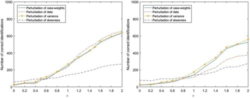
From Figure 1 (left), we see clearly that the number of samples with correct identification of the influential observation has followed the scale of the perturbed vector to increase in the four perturbation strategies. When $ϵ=2$, the four strategies are becoming apparent. Under 1000 samples, the influential observation of the four schemes are 634, 658, 642 and 269 times, respectively. These results are expected.

Next, we further study the STAR(2) model stated as $y_t={\text{β}}_1{y}_{t-1}+{\text{β}}_2{y}_{t-2}+u_t$, where $u_t\sim \mathrm{ST}(0,{\sigma }^2,\lambda ,\varsigma )$, with ${\text{β}}_1=0.15,{\text{β}}_2=-0.2,{\sigma }^2=0.1,\lambda =0.2,\varsigma =3$. It is easy to prove that the AR(2) model is stationary. We use the same 5 steps for the AR(1) model to get Figure 1 (right).

From Figure 1 (right), we note that the number of samples with correct identification of the influential observation has follewed the scale of the perturbed vector to increase in the four schemes. When $ϵ=2$, the four schemes become apparent. Under 1000 samples, the influential observation of the four schemes are 525, 375, 561 and 277 times, respectively. From both figures, the AR(1) model's pattern appears stronger than the AR(2) model's patter. However, diagnostic ability of the four schemes are different so they should be used in combination in practice.

4.3. Student-t versus Gaussian models

Liu et al.[26] investigated about a methodology to detect influential points in an AR model with the normal distribution. Here, we generate 1000 samples following the procedure provided in Section 4.2 (with $ϵ=2$ in [3]) based on the ST distribution with $\text{β}=0.12,{\sigma }^2=0.1,\lambda =0.2,\varsigma =3$, and then make an influence analysis under the ST and normal distributions to compare our result with those provided in [26]. Using the method stated in Step 5 of Section 4.2, the comparison is made in Table 3.

Table 3. Comparison between the ST and normal distributions with ε = 2.

Number of correct outlier detections	Case-weights	Data	Variance
Local influence under the ST distribution	634	658	642
Local influence under the normal distribution	603	596	122

There are both similarities and differences. The similarities are obvious in the study under both distributions as the number of correct outlier detections are all large, that is, 634, 658, 642 and 603, 596, 122 out of 1000. This indicates that the diagnostic results works well. However, there are also differences. In the case of $ϵ=2$, the number of 1000 samples with influential points is 634 and 603 under case-weights strategy; the number of 1000 samples with influential points is 658 and 596 under the data strategy; and the number of 1000 samples with influential points is 642 and 122 under the variance strategy. In terms of diagnostics, the ST model is better than the normal model. Utilizing a correctly specified model in analyzing data is particularly important.

4.4. Skew-student-t versus student-t models

Liu et al. [34] diagnosed influential points in an AR model with the t distribution. We generate 1000 samples following the procedure provided in Section 4.2 (with ε = 2 in Step 3) based on the ST distribution with $\text{β}=0.12,{\sigma }^2=0.1,\lambda =0.2,\varsigma =3$ to evaluate the performance of local influence analysis under the ST and t distributions. The comparison is reported in Table 4. The number of samples where influential observations were detected are all large in scale, namely, 634, 658 and 637, 613 out of 1000, implying that the method works well. There are differences in employing the ST and t distributions. In the case of $ϵ=2$, the number of samples with influential observations is 634 and 658 under case weights strategy; and the number of samples with influential observations is 658 and 613 under the data strategy; both with a total 1000 samples. The diagnostic effect under the ST distribution is better than under the t distribution.

Table 4. Comparison between the ST and t distributions with ε = 2.

Number of correct outlier detections	Case-weights	Data
Local influence under ST distribution	634	658
Local influence under t distribution	637	613

4.5. Skew-student-t versus skew-normal models

Liu et al. [31,32] detected influential observations in an SNAR model. We generate 1000 samples following the procedure provided in Section 4.2 (with $ϵ=2$ in Step 3) based on the ST distribution with $\text{β}=0.12,{\sigma }^2=0.1,\lambda =0.2,\varsigma =3$, and then apply a local influence analysis under the ST and SN distributions. The comparison is provided in Table 5.

Table 5. Comparison between the ST and SN distributions with $ϵ=2$.

Number of correct outlier detections	Case-weights	Data	Variance	Skewness
Local influence under ST distribution	634	658	642	269
Local influence under SN distribution	611	609	124	46

The similarities are noticeable in the local diagnostic study under the ST and SN models as the number of samples with the influential points are most large enough in the most strategies of perturbation: 634, 658, 642, 269 and 611, 609, 124, 46 out of 1000, meaning that the diagnostic results are effective. However, there are also differences. In the case of $ϵ=2$, these can be observed for the variance and skewness perturbation strategies, which influential observations are 642 and 124 under the variance strategy; and 269 and 46 under the skewness strategy; both with a total 1000 samples. The local influence analysis performance is better assuming a ST distribution that an SN distribution, as shown in the previous cases.

5. Empirical analysis

In this section, we use our values stated in Section 3 to analyze financial data and discuss the performance of our proposed methodology. The Brent crude futures (BIPE hereafter) daily log-return data from 16 January 2007 to 11 March 2021 are chosen to construct an STAR model and perform our diagnostic analysis.

5.1. STAR model for BIPE

Figure 2 (left) shows BIPE daily log-return time series data from 16 January 2007 to 11 March 2021. An exploratory data analysis based on basic statistics of the daily financial returns is the following: n = 3442 (sample size); minimum and maximum returns of −0.30856 and 0.15449; first and third quartiles of −0.010586 and 0.011026; sample mean and median of 0.0000669 and 0.00013246; sample coefficient of skewness of −0.93637; and sample excess kurtosis of 18.812. Figures 2 (right) and 3 present a histogram and a kernel plot employing the t model of the BIPE daily data. From this exploratory data analysis, we detect an asymmetrical distributional feature and a high kurtosis level of the data. We can observe that the adjustment with the t model is unsuitable. Furthermore, we use the D'Agostino skewness test [10] and Anscombe-Glynn kurtosis test [1] to assess for skewness and kurtosis of our data, where the D'Agostino statistic is -19.25 and Anscombe-Glynn statistic is 27.754, with their p-values both significantly less than 0.01. These indicate that the distribution of BIPE is skewed, with an obvious peak and two fat tails. We first select an STAR model and determine its order using the following steps as stated as [31,32,47] for their t and SN models.

Figure 2. Time-series (left) and histogram with kernel PDF (right) of BIPE daily returns.

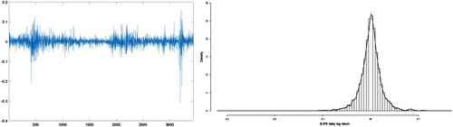
Figure 3. BIPE daily returns with t and ST PDFs.

[S1] Consider an AR(p) model (18) $\begin{array}{l}{y}_t=u_t+{\text{β}}_1{y}_{t-1},\\ ⋮\\ y_t=u_t+{\text{β}}_1{y}_{t-1}+\cdots +{\text{β}}_p{y}_{t-p},\\ ⋮\end{array}$(18) with $p\in \{1,2,\dots \}$.

[S2] In the ith equation of (19(18) $\begin{array}{l}{y}_t=u_t+{\text{β}}_1{y}_{t-1},\\ ⋮\\ y_t=u_t+{\text{β}}_1{y}_{t-1}+\cdots +{\text{β}}_p{y}_{t-p},\\ ⋮\end{array}$(18) ), that is, the AR(i) model, the ordinary least squares estimate of ${\text{β}}_j$ is ${\widehat{\text{β}}}_j^{\left(i\right)}$, the residual is ${\hat{u}}_t^{\left(i\right)}=y_t-{\widehat{\text{β}}}_1^{\left(i\right)}{y}_{t-1}-\cdots -{\widehat{\text{β}}}_i^{\left(i\right)}{y}_{t-i},$ and the estimate of ${\sigma }_i^2$ is ${\hat{\sigma }}_i^2=\frac{1}{R-2i-1}\sum _{t=i+1}^R{\left({\hat{u}}_t^{\left(i\right)}\right)}^2.$

[S3] The $(i-1)$th and ith equations in (19(18) $\begin{array}{l}{y}_t=u_t+{\text{β}}_1{y}_{t-1},\\ ⋮\\ y_t=u_t+{\text{β}}_1{y}_{t-1}+\cdots +{\text{β}}_p{y}_{t-p},\\ ⋮\end{array}$(18) ) are used to test if coefficient ${\text{β}}_i$ is equal to zero or not, that is, to compare the AR(i−1) with AR(i) models. For this hypothesis testing the statistic is stated as $T_i=-(R-i-2.5)\ln \left({\hat{\sigma }}_i^2/{\hat{\sigma }}_{i-1}^2\right)$, which follows an asymptotic ${\chi }^2\left(1\right)$ distribution. Values of $T_i$ for $i\in \{1,\dots ,7\}$ are presented in Table 6. As the 95% quantile of ${\chi }^2\left(1\right)$ distribution is 3.841, we use the empirical values of $T_i$ presented in Table 6 to determine the value of p of the AR(p) model. Hence, p = 1 because $T_i=3.863>3.841$. Using the EM algorithm, we calculate $\hat{\mathbf{\Theta }}=(\widehat{{\text{β}}_1},{\hat{\sigma }}^2,\hat{\lambda },\hat{\varsigma })=(-0.07232,0.000201,0.024942,3)$. Then, as the absolute value of ${\text{β}}_1$ is less than one, we cannot reject the BIPE data to be stationary. From Figure 3, we find that the ST distribution fits better than the t distribution. Thus, we fit the STAR(1) model ${\hat{y}}_t=-0.07232y_{t-1}+{\hat{u}}_t$, with ${\hat{\sigma }}^2=0.000201$, $\hat{\lambda }=0.024942$, and $\hat{\varsigma }=3$. According to Lemma 1, the data being fitted by the STAR(1) model are stationary.

Table 6. Empirical values of $T_i$, with $i\in \{1,\dots ,7\}$ for BIPE daily data.

i	1	2	3	4	5	6	7
$T_i$	3.863	−1.708	−1.878	3.205	−1.940	−1.675	−1.996

5.2. Diagnostic analysis for BIPE

We conduct the local influence analysis in the STAR(1) model for BIPE under the four perturbation strategies proposed. Based on the idea given in Section 3.3 and the results in [31,32], we choose c = 3 and $1/3441+3{\mathrm{SD}}_{M\left(0\right)}$ as the benchmark, obtaining the values of 0.0021, 0.0022, 0.0015 and 0.0012 for the four respective perturbation strategies. In each plot, the red line symbolizes the benchmark to determine if an observation to be potentially influential or not, that is, when its value is beyond the red line. The influential observations are in Table 7 where * denotes the case that is identified as potentially influential for BIPE. We can observe that these cases are mainly related to the 2008–2009 ‘The Great Recession”, as well as to the 2020-2021 SARS-CoV-2 pandemic, which conducted to a large volatility. For example, on 3 October 2008, the U.S. government signed a financial rescue plan with a total of about 700 billion dollars. On 24 February 2020, the global stock markets fell after the global number of COVID-19 cases increased significantly. In summary, Figure 4 and Table 7 justify the effectiveness and practicability of the diagnostics methods for an STAR model.

Figure 4. BIPE diagnostics under skewness, variance, case-weights, and data perturbations.

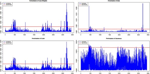
Table 7. Summary of the diagnostic analysis by perturbation strategy.

Date	Case-weights	Data	Variance	Skewness	Date	Case-weights	Data	Variance	Skewness	Date	Case-weights	Data	Variance	Skewness
2008/5/6					2009/2/3					2016/2/18			*
2008/6/10					2009/3/2					2016/8/12			*
2008/9/16				*	2009/3/3	*		*		2016/12/1			*
2008/9/17					2009/3/13					2018/11/20
2008/9/23					2009/3/30					2018/12/27			*
2008/10/6				*	2009/3/31	*		*		2019/9/17			*
2008/10/7					2009/4/3	*		*		2020/2/3
2008/10/10				*	2009/4/10					2020/2/4			*
2008/10/13					2009/4/20					2020/3/3			*
2008/10/16				*	2009/6/2					2020/3/6
2008/10/17					2009/9/1					2020/3/9
2008/10/22				*	2010/2/23					2020/3/10			*
2008/10/23					2011/5/5					2020/3/11			*
2008/10/30					2011/5/6	*		*		2020/3/16
2008/11/3				*	2011/12/23					2020/3/17			*
2008/11/5				*	2015/1/5					2020/3/18
2008/11/6				*	2015/1/6	*		*		2020/3/19			*
2008/11/7					2015/2/2	*		*		2020/3/30
2008/11/20				*	2015/3/19			*		2020/3/31			*
2008/11/21					2015/4/8	*		*		2020/4/3			*
2008/11/25					2015/7/6					2020/4/7			*
2008/12/1				*	2015/8/24					2020/4/8			*
2008/12/2					2015/8/25	*				2020/4/15
2008/12/4				*	2015/8/28	*		*		2020/4/20			*
2008/12/9					2015/9/1	*		*		2020/4/21
2008/12/12					2015/9/2	*		*		2020/4/22			*
2008/12/24				*	2015/10/9					2020/4/27
2008/12/25					2016/1/7	*				2020/4/28
2009/1/5					2016/1/12	*				2020/5/7			*
2009/1/6					2016/1/18	*				2020/5/15			*
2009/1/7				*	2016/1/22			*		2020/5/19			*
2009/1/8					2016/1/25	*		*		2020/6/11
2009/1/12					2016/1/28			*		2020/6/12
2009/2/2				*	2016/2/4	*		*		2020/11/10			*

Finally, we compare the two models for AR(1) with outliers and STAR(1) without outliers in Table 8. The two models’ mean square errors of their predicted values are 0.0014874 and 0.0013266, respectively. It can be seen that the prediction results made after the outliers' removal are better than those made before.

Table 8. Predicted results by the listed structure.

Date	BIPE returns	AR(1) model	STAR(1) model
2021/2/26	−0.0217	0.0002	0.0497
2021/3/1	−0.0206	0.0280	−0.0391
2021/3/2	−0.0110	−0.0096	−0.0133
2021/3/3	0.0216	0.0099	0.0127
2021/3/4	0.0498	−0.0161	0.0953
2021/3/5	0.0355	−0.0278	0.0636
2021/3/8	−0.0228	−0.0095	0.0201
2021/3/9	−0.0121	0.0074	0.0078

6. Conclusions

In this article, our STAR model was studied with an ML estimation methodology. Its validation was performed using local diagnostic analysis inspired by the EM algorithm, which allowed us to obtain normal curvatures for four perturbation strategies of interest. Our model was compared with the alternative models based on skew-normal, normal, and Student-t distributions. Our findings showed that the proposed STAR model was more accurate, applicable, and usable to diagnose longer time data and identify more abnormal cases.

The curvature results for our STAR(p) model with four perturbation strategies, including the newly proposed perturbation of skewness, were presented. Monte Carlo simulation studies were conducted to asses adequacy of our methodology. Approximate numerical benchmark values for detecting the possible influential observations were employed to analyze the daily log-returns of Brent crude futures for a period of time covering the events related to 2008 financial crisis and COVID-19 pandemic. Many of the influential observations with the BIPE data were identified to be related to historical events. Our methodology and findings are evidenced to be effective.

Further works are related to the study of statistical structures generated from settings associated with data functional, partial least squares, quantile, multivariate, and spatial regression frameworks [16,38,39,43]. Similarly, considering censored data may also be of interest to analyze in the context of the current investigation [19]. We are planning to conduct studies on these issues in the future.

Acknowledgments

We would like to thank the Editor, Professor Jie Chen, the Associate Editor, and the reviewers for their constructive comments which led an improved presentation of this article.

Disclosure statement

No potential conflict of interest was reported by the author(s).

Additional information

Funding

The research of Y. Liu was supported by the National Social Science Fund of China [grant No. 19BTJ036]. The research of V. Leiva was partially funded by the National Agency for Research and Development (ANID) [project grant number FONDECYT 1200525] of the Chilean government under the Ministry of Science, Technology, Knowledge, and Innovation.

Appendix

In this appendix, we obtain the matrix derivatives involved in our diagnostic analytics [18,28,37].

A.1 Proof (Theorem 1)

Proof.

The Q-function is established as $\begin{array}{rl}{Q}_{\mathbf{\Theta }}& =\sum _{i=p+1}^R(-\frac{\varsigma }{2}{\hat{s}}_{1i}-\frac{{u_i}^2{\hat{s}}_{1i}}{2(1-{{\delta }_{\lambda }}^2)\widehat{{\sigma }^2}}+\frac{{\delta }_{\lambda }{u}_i{\hat{s}}_{2i}}{(1-{{\delta }_{\lambda }}^2){\sigma }^2}-\frac{{\hat{s}}_{3i}}{2(1-{{\delta }_{\lambda }}^2){\sigma }^2}\\ & -\ln \left({\sigma }^2\right)-\frac{1}{2}\ln (1-{{\delta }_{\lambda }}^2)+\frac{\varsigma }{2}\ln \left(\frac{\varsigma }{2}\right)-\ln \left(\mathrm{\Gamma }\left(\frac{\varsigma }{2}\right)\right)+\frac{\varsigma }{2}{\hat{s}}_{4i}).\end{array}$ Its derivatives are expressed as $\begin{array}{rl}\frac{\mathrm{\partial }{Q}_{\mathbf{\Theta }}}{\mathrm{\partial }\text{β}}& =\sum _{i=p+1}^R\frac{u_i{\hat{s}}_{1i}-{\delta }_{\lambda }{\hat{s}}_{2i}}{(1-{{\delta }_{\lambda }}^2){\sigma }^2}{\mathit{x}}_i^{\mathrm{\top }},\frac{\mathrm{\partial }{Q}_{\mathbf{\Theta }}}{\mathrm{\partial }{\sigma }^2}=\sum _{i=p+1}^R\frac{{u_i}^2{\hat{s}}_{1i}-2{\delta }_{\lambda }{u}_i{\hat{s}}_{2i}+{\hat{s}}_{3i}}{2(1-{{\delta }_{\lambda }}^2){\sigma }^4}-\frac{1}{{\sigma }^2},\\ \frac{\mathrm{\partial }{Q}_{\mathbf{\Theta }}}{\mathrm{\partial }{\delta }_{\lambda }}& =\sum _{i=p+1}^R(\frac{{\delta }_{\lambda }}{1-{{\delta }_{\lambda }}^2}+\frac{-{\delta }_{\lambda }{u_i}^2{\hat{s}}_{1i}+2{{\delta }_{\lambda }}^2{u}_i{\hat{s}}_{2i}+(1-{{\delta }_{\lambda }}^2)u_i{\hat{s}}_{2i}-{\delta }_{\lambda }{\hat{s}}_{3i}}{{(1-{{\delta }_{\lambda }}^2)}^2{\sigma }^2}),\\ \frac{\mathrm{\partial }{Q}_{\mathbf{\Theta }}}{\mathrm{\partial }\varsigma }& =\frac{R-p}{2}(1-{\hat{s}}_{1i}+{\hat{s}}_{4i}+\ln \left(\frac{\varsigma }{2}\right)-G\left(\frac{\varsigma }{2}\right)).\end{array}$ The second derivatives are formulated as $\begin{array}{rl}\frac{{\mathrm{\partial }}^2{Q}_{\mathbf{\Theta }}}{\mathrm{\partial }\text{β}\mathrm{\partial }{\text{β}}^{\mathrm{\top }}}& =-\sum _{i=p+1}^R\frac{{\hat{s}}_{1i}}{(1-{{\delta }_{\lambda }}^2){\sigma }^2}{{\mathit{x}}_i}^{\mathrm{\top }}{\mathit{x}}_i,\frac{{\mathrm{\partial }}^2{Q}_{\mathbf{\Theta }}}{\mathrm{\partial }\text{β}\mathrm{\partial }{\sigma }^2}=\sum _{i=p+1}^R\frac{{\delta }_{\lambda }{\hat{s}}_{2i}-u_i{\hat{s}}_{1i}}{(1-{{\delta }_{\lambda }}^2){\sigma }^4}{{\mathit{x}}_i}^{\mathrm{\top }},\\ \frac{{\mathrm{\partial }}^2{Q}_{\mathbf{\Theta }}}{\mathrm{\partial }\text{β}\mathrm{\partial }{\delta }_{\lambda }}& =\sum _{i=p+1}^R\frac{2{\delta }_{\lambda }{u}_i{\hat{s}}_{1i}-({{\delta }_{\lambda }}^2+1){\hat{s}}_{2i}}{{(1-{{\delta }_{\lambda }}^2)}^2{\sigma }^2}{{\mathit{x}}_i}^{\mathrm{\top }},\\ \frac{{\mathrm{\partial }}^2{Q}_{\mathbf{\Theta }}}{\mathrm{\partial }{\left({\sigma }^2\right)}^2}& =\sum _{i=p+1}^R(\frac{-{u_i}^2{\hat{s}}_{1i}+2{\delta }_{\lambda }{u}_i{\hat{s}}_{2i}-{\hat{s}}_{3i}}{(1-{{\delta }_{\lambda }}^2){\sigma }^6}+\frac{1}{{\sigma }^4}),\\ \frac{{\mathrm{\partial }}^2{Q}_{\mathbf{\Theta }}}{\mathrm{\partial }{\sigma }^2\mathrm{\partial }{\delta }_{\lambda }}& =\sum _{i=p+1}^R\frac{{\delta }_{\lambda }{u_i}^2{\hat{s}}_{1i}-({{\delta }_{\lambda }}^2+1)u_i{\hat{s}}_{2i}+{\delta }_{\lambda }{\hat{s}}_{3i}}{{(1-{{\delta }_{\lambda }}^2)}^2{\sigma }^4},\\ \frac{{\mathrm{\partial }}^2{Q}_{\mathbf{\Theta }}}{\mathrm{\partial }{{\delta }_{\lambda }}^2}& =\sum _{i=p+1}^R(\frac{{{\delta }_{\lambda }}^2+1}{{(1-{{\delta }_{\lambda }}^2)}^2}+\frac{-{u_i}^2{\hat{s}}_{1i}+6{\delta }_{\lambda }{u}_i{\hat{s}}_{2i}-{\hat{s}}_{3i}}{{(1-{{\delta }_{\lambda }}^2)}^2{\sigma }^2}+\frac{-4{{\delta }_{\lambda }}^2{u_i}^2{\hat{s}}_{1i}+8{{\delta }_{\lambda }}^3{u}_i{\hat{s}}_{2i}+4{{\delta }_{\lambda }}^2{\hat{s}}_{3i}}{{(1-{{\delta }_{\lambda }}^2)}^3{\sigma }^{{\sigma }^2}}),\\ \frac{{\mathrm{\partial }}^2{Q}_{\mathbf{\Theta }}}{\mathrm{\partial }{\delta }_{\lambda }\mathrm{\partial }\varsigma }& =\frac{{\mathrm{\partial }}^2{Q}_{\mathbf{\Theta }}}{\mathrm{\partial }\text{β}\mathrm{\partial }\varsigma }=\frac{{\mathrm{\partial }}^2{Q}_{\mathbf{\Theta }}}{\mathrm{\partial }{\sigma }^2\mathrm{\partial }\varsigma }=0,\frac{{\mathrm{\partial }}^2{Q}_{\mathbf{\Theta }}}{\mathrm{\partial }{\varsigma }^2}=\frac{R-p}{4}(\frac{2}{\varsigma }-G^{\prime }\left(\frac{\varsigma }{2}\right)).\end{array}$ Hence, we obtain ${\ddot{Q}}_{\hat{\mathbf{\Theta }}}$ with $\hat{\mathbf{\Theta }}=(\widehat{\text{β}},{\hat{\sigma }}^2,\widehat{{\mathit{\delta }}_{\lambda }},\hat{\varsigma })$.

A.2. Proof (Theorem 2)

Proof.

The Q-function (perturbed) is stated as $\begin{array}{rl}{Q}_{\mathbf{\Theta };\mathit{\omega }}& =\sum _{i=p+1}^R(-\frac{\varsigma }{2}{\hat{s}}_{1i}-\frac{{\omega }_i^2{u_i}^2{\hat{s}}_{1i}}{2(1-{{\delta }_{\lambda }}^2){\sigma }^2}+\frac{{\delta }_{\lambda }{\omega }_i{u}_i{\hat{s}}_{2i}}{(1-{{\delta }_{\lambda }}^2){\sigma }^2}-\frac{{\hat{s}}_{3i}}{2(1-{{\delta }_{\lambda }}^2){\sigma }^2}\\ & -\ln \left({\sigma }^2\right)-\frac{1}{2}\ln (1-{{\delta }_{\lambda }}^2)+\frac{\varsigma }{2}\ln \left(\frac{\varsigma }{2}\right)-\ln \left(\mathrm{\Gamma }\left(\frac{\varsigma }{2}\right)\right)+\frac{\varsigma }{2}{\hat{s}}_{4i}).\end{array}$ Taking the differentials of the Q-function (perturbed) with respect to $\text{β}$, ${\sigma }^2$, ${\delta }_{\lambda }$, ς and then ${\omega }_i$, for $i\in \{p+1,\dots ,R\}$, the derivatives are calculated as $\begin{array}{rl}\frac{\mathrm{\partial }{Q}_{\mathbf{\Theta };\mathit{\omega }}}{\mathrm{\partial }\text{β}}& =\sum _{i=p+1}^R\frac{u_i{w_i}^2{\hat{s}}_{1i}-{\delta }_{\lambda }{w}_i{\hat{s}}_{2i}}{(1-{{\delta }_{\lambda }}^2){\sigma }^2}{\mathit{x}}_i^{\mathrm{\top }},\frac{\mathrm{\partial }{Q}_{\mathbf{\Theta };\mathit{\omega }}}{\mathrm{\partial }{\sigma }^2}=\sum _{i=p+1}^R(\frac{{w_i}^2{u_i}^2{\hat{s}}_{1i}-2{\delta }_{\lambda }{w}_i{u}_i{\hat{s}}_{2i}+{\hat{s}}_{3i}}{2(1-{{\delta }_{\lambda }}^2){\sigma }^4}-\frac{1}{{\sigma }^2}),\\ \frac{\mathrm{\partial }{Q}_{\mathbf{\Theta };\mathit{\omega }}}{\mathrm{\partial }{\delta }_{\lambda }}& =\sum _{i=p+1}^R(\frac{{\delta }_{\lambda }}{1-{{\delta }_{\lambda }}^2}+\frac{-{\delta }_{\lambda }{w_i}^2{u_i}^2{\hat{s}}_{1i}+2{{\delta }_{\lambda }}^2{w}_i{u}_i{\hat{s}}_{2i}+(1-{{\delta }_{\lambda }}^2)w_i{u}_i{\hat{s}}_{2i}-{\delta }_{\lambda }{\hat{s}}_{3i}}{{(1-{{\delta }_{\lambda }}^2)}^2{\sigma }^2}),\\ \frac{\mathrm{\partial }{Q}_{\mathbf{\Theta };\mathit{\omega }}}{\mathrm{\partial }\varsigma }& =\frac{R-p}{2}(1-{\hat{s}}_{1i}+{\hat{s}}_{4i}+\ln \left(\frac{\varsigma }{2}\right)-G\left(\frac{\varsigma }{2}\right)),\end{array}$ and the second derivatives are stated as $\begin{array}{rl}\frac{{\mathrm{\partial }}^2{Q}_{\mathbf{\Theta };\mathit{\omega }}}{\mathrm{\partial }\text{β}\mathrm{\partial }{\omega }_i}& =\frac{2w_i{u}_i{\hat{s}}_{1i}-{\delta }_{\lambda }{\hat{s}}_{2i}}{(1-{{\delta }_{\lambda }}^2){\sigma }^2}{\mathit{x}}_i^{\mathrm{\top }},\frac{{\mathrm{\partial }}^2{Q}_{\mathbf{\Theta };\mathit{\omega }}}{\mathrm{\partial }{\sigma }^2\mathrm{\partial }{\omega }_i}=\frac{w_i{u_i}^2{\hat{s}}_{1i}-{\delta }_{\lambda }{u}_i{\hat{s}}_{2i}}{(1-{{\delta }_{\lambda }}^2){\sigma }^2},\\ \frac{{\mathrm{\partial }}^2{Q}_{\mathbf{\Theta };\mathit{\omega }}}{\mathrm{\partial }{\delta }_{\lambda }\mathrm{\partial }{\omega }_i}& =\frac{-2{\delta }_{\lambda }{w}_i{u_i}^2{\hat{s}}_{1i}+{{\delta }_{\lambda }}^2{u}_i{\hat{s}}_{2i}+u_i{\hat{s}}_{2i}}{{(1-{{\delta }_{\lambda }}^2)}^2{\sigma }^2},\frac{{\mathrm{\partial }}^2{Q}_{\mathbf{\Theta };\mathit{\omega }}}{\mathrm{\partial }\varsigma \mathrm{\partial }{\omega }_i}=0.\end{array}$ Letting $\hat{\mathbf{\Theta }}=(\widehat{\text{β}},\widehat{{\sigma }^2},\widehat{{\mathit{\delta }}_{\lambda }},\hat{\varsigma })$ and $\mathit{\omega }=(1,\dots ,1{)}^{\mathrm{\top }}$, we obtain the expression presented in (11(10) $\begin{array}{rl}{Q}_{\mathbf{\Theta };\mathit{\omega }}& =\mathrm{E}\left({\ell }_{\mathrm{complete}}\right(\mathbf{\Theta };\mathit{\omega };{\mathit{Y}}_{\mathrm{complete}}\left)|{\mathit{y}}_o\right),\mathrm{evaluated}\mathrm{at}\mathbf{\Theta }\equiv \hat{\mathbf{\Theta }},\\ & =\sum _{i=p+1}^R(-\frac{\varsigma }{2}{\hat{s}}_{1i}-\frac{{\omega }_i^2{u}_i^2{\hat{s}}_{1i}}{2(1-{\delta }_{\lambda }^2){\sigma }^2}+\frac{{\delta }_{\lambda }{\omega }_i{u}_i{\hat{s}}_{2i}}{(1-{{\delta }_{\lambda }}^2){\sigma }^2}-\frac{{\hat{s}}_{3i}}{2(1-{{\delta }_{\lambda }}^2){\sigma }^2}\\ & -\ln \left({\sigma }^2\right)-\frac{1}{2}\ln (1-{{\delta }_{\lambda }}^2)+\frac{\varsigma }{2}\ln \left(\frac{\varsigma }{2}\right)-\ln \left(\mathrm{\Gamma }\left(\frac{\varsigma }{2}\right)\right)+\frac{\varsigma }{2}{\hat{s}}_{4i}),\end{array}$(10) ).

A.3. Proof (Theorem 3)

Proof.

We get the $Q$-function (perturbed) $\begin{array}{rl}{Q}_{\mathbf{\Theta };\mathit{\omega }}& =\sum _{i=p+1}^R(-\frac{\varsigma }{2}{\hat{s}}_{1i}-\frac{(u_i+\mu ({\omega }_i){)}^2{\hat{s}}_{1i}}{2(1-{{\delta }_{\lambda }}^2){\sigma }^2}+\frac{{\delta }_{\lambda }(u_i+\mu ({\omega }_i\left)\right){\hat{s}}_{2i}}{(1-{{\delta }_{\lambda }}^2){\sigma }^2}-\frac{{\hat{s}}_{3i}}{2(1-{{\delta }_{\lambda }}^2){\sigma }^2}\\ & -\ln \left({\sigma }^2\right)-\frac{1}{2}\ln (1-{{\delta }_{\lambda }}^2)+\frac{\varsigma }{2}\ln \left(\frac{\varsigma }{2}\right)-\ln \left(\mathrm{\Gamma }\left(\frac{\varsigma }{2}\right)\right)+\frac{\varsigma }{2}{\hat{s}}_{4i}).\end{array}$ Taking the differentials of the Q-function (perturbed) with respect to $\text{β}$, ${\sigma }^2$, ${\delta }_{\lambda }$, ς and then ${\omega }_i$, for $i\in \{p+1,\dots ,R\}$, the derivatives are found by $\begin{array}{rl}\frac{\mathrm{\partial }{Q}_{\mathbf{\Theta };\mathit{\omega }}}{\mathrm{\partial }\text{β}}& =\sum _{i=p+1}^R\frac{(u_i+\mu ({\omega }_i\left)\right){\hat{s}}_{1i}-{\delta }_{\lambda }{\hat{s}}_{2i}}{(1-{{\delta }_{\lambda }}^2){\sigma }^2}({{\mathit{x}}_i}^{\mathrm{\top }}+{({\omega }_{i-1},\dots ,{\omega }_{i-p})}^{\mathrm{\top }}),\\ \frac{\mathrm{\partial }{Q}_{\mathbf{\Theta };\mathit{\omega }}}{\mathrm{\partial }{\sigma }^2}& =\sum _{i=p+1}^R(\frac{{(u_i+\mu ({\omega }_i\left)\right)}^2{\hat{s}}_{1i}-2{\delta }_{\lambda }(u_i+\mu ({\omega }_i\left)\right){\hat{s}}_{2i}+{\hat{s}}_{3i}}{2(1-{{\delta }_{\lambda }}^2){\sigma }^4}-\frac{1}{{\sigma }^2}),\\ \frac{\mathrm{\partial }{Q}_{\mathbf{\Theta };\mathit{\omega }}}{\mathrm{\partial }{\delta }_{\lambda }}& =\sum _{i=p+1}^R(\frac{{\delta }_{\lambda }}{1-{{\delta }_{\lambda }}^2}+\frac{-{\delta }_{\lambda }{(u_i+\mu ({\omega }_i\left)\right)}^2{\hat{s}}_{1i}+({{\delta }_{\lambda }}^2+1)(u_i+\mu ({\omega }_i\left)\right){\hat{s}}_{2i}-{\delta }_{\lambda }{\hat{s}}_{3i}}{(1-{{\delta }_{\lambda }}^2){\sigma }^2}),\\ \frac{\mathrm{\partial }{Q}_{\mathbf{\Theta };\mathit{\omega }}}{\mathrm{\partial }\varsigma }& =\frac{R-p}{2}(1-{\hat{s}}_{1i}+{\hat{s}}_{4i}+\ln \left(\frac{\varsigma }{2}\right)-G\left(\frac{\varsigma }{2}\right)),\end{array}$ and the second derivatives are established as $\begin{array}{rl}\frac{{\mathrm{\partial }}^2{Q}_{\mathbf{\Theta };\mathit{\omega }}}{\mathrm{\partial }\text{β}\mathrm{\partial }{\omega }_i}& =\frac{{\hat{s}}_{1i}}{(1-{{\delta }_{\lambda }}^2){\sigma }^2}({{\mathit{x}}_i}^{\mathrm{\top }}+{({\omega }_{i-1},\dots ,{\omega }_{i-p})}^{\mathrm{\top }}),\frac{{\mathrm{\partial }}^2{Q}_{\mathbf{\Theta };\mathit{\omega }}}{\mathrm{\partial }{\sigma }^2\mathrm{\partial }{\omega }_i}=\frac{(u_i+\mu ({\omega }_i\left)\right){\hat{s}}_{1i}-{\delta }_{\lambda }{\hat{s}}_{2i}}{(1-{{\delta }_{\lambda }}^2){\sigma }^4},\\ \frac{{\mathrm{\partial }}^2{Q}_{\mathbf{\Theta };\mathit{\omega }}}{\mathrm{\partial }{\delta }_{\lambda }\mathrm{\partial }{\omega }_i}& =\frac{({{\delta }_{\lambda }}^2+1){\hat{s}}_{2i}-2{\delta }_{\lambda }(u_i+\mu ({\omega }_i\left)\right){\hat{s}}_{1i}}{{(1-{{\delta }_{\lambda }}^2)}^2{\sigma }^2},\frac{{\mathrm{\partial }}^2{Q}_{\mathbf{\Theta };\mathit{\omega }}}{\mathrm{\partial }\varsigma \mathrm{\partial }{\omega }_i}=0.\end{array}$ Noting $\hat{\mathbf{\Theta }}=(\widehat{\text{β}},{\hat{\sigma }}^2,\widehat{{\mathit{\delta }}_{\lambda }},\hat{\varsigma })$ and $\mathit{\omega }=(0,\dots ,0{)}^{\mathrm{\top }}$, we reach the formula given in (13(12) $\begin{array}{rl}{Q}_{\mathbf{\Theta };\mathit{\omega }}& =\sum _{i=p+1}^R(-\frac{\varsigma }{2}{\hat{s}}_{1i}-\frac{(u_i+\mu ({\omega }_i){)}^2{\hat{s}}_{1i}}{2(1-{{\delta }_{\lambda }}^2){\sigma }^2}+\frac{{\delta }_{\lambda }(u_i+\mu ({\omega }_i\left)\right){\hat{s}}_{2i}}{(1-{{\delta }_{\lambda }}^2){\sigma }^2}-\frac{{\hat{s}}_{3i}}{2(1-{{\delta }_{\lambda }}^2){\sigma }^2}\\ & -\ln \left({\sigma }^2\right)-\frac{1}{2}\ln (1-{{\delta }_{\lambda }}^2)+\frac{\varsigma }{2}\ln \left(\frac{\varsigma }{2}\right)-\ln \left(\mathrm{\Gamma }\left(\frac{\varsigma }{2}\right)\right)+\frac{\varsigma }{2}{\hat{s}}_{4i}),\end{array}$(12) ).

A.4. Proof (Theorem 4)

Proof.

We attain Q-function (perturbed) $\begin{array}{rl}{Q}_{\mathbf{\Theta };\mathit{\omega }}& =\sum _{i=p+1}^{\mathrm{\top }}(-\frac{\varsigma }{2}{\hat{s}}_{1i}-\frac{{\omega }_i{u_i}^2{\hat{s}}_{1i}}{2(1-{{\delta }_{\lambda }}^2){\sigma }^2}+\frac{{\delta }_{\lambda }{\omega }_i{u}_i{\hat{s}}_{2i}}{(1-{{\delta }_{\lambda }}^2){\sigma }^2}-\frac{{\omega }_i{\hat{s}}_{3i}}{2(1-{{\delta }_{\lambda }}^2){\sigma }^2}\\ & -\ln \left(\frac{{\sigma }^2}{{\omega }_i}\right)-\frac{1}{2}\ln (1-{{\delta }_{\lambda }}^2)+\frac{\varsigma }{2}\ln \left(\frac{\varsigma }{2}\right)-\ln \left(\mathrm{\Gamma }\left(\frac{\varsigma }{2}\right)\right)+\frac{\varsigma }{2}{\hat{s}}_{4i}).\end{array}$ Taking the differentials of the Q-function (perturbed) with respect to $\text{β}$, ${\sigma }^2$, ${\delta }_{\lambda }$, ς and then ${\omega }_i$, for $i\in \{p+1,\dots ,R\}$, the derivatives are stated as $\begin{array}{rl}\frac{\mathrm{\partial }{Q}_{\mathbf{\Theta };\mathit{\omega }}}{\mathrm{\partial }\text{β}}& =\sum _{i=p+1}^R{w}_i\frac{{\hat{s}}_{1i}{u}_i-{\delta }_{\lambda }{\hat{s}}_{2i}}{(1-{{\delta }_{\lambda }}^2){\sigma }^2}{{\mathit{x}}_i}^{\mathrm{\top }},\frac{\mathrm{\partial }{Q}_{\mathbf{\Theta };\mathit{\omega }}}{\mathrm{\partial }{\sigma }^2}=\sum _{i=p+1}^R(w_i\frac{{u_i}^2{\hat{s}}_{1i}-2{\delta }_{\lambda }{u}_i{\hat{s}}_{2i}+{\hat{s}}_{3i}}{2(1-{{\delta }_{\lambda }}^2){\sigma }^4}-\frac{1}{{\sigma }^2}),\\ \frac{\mathrm{\partial }{Q}_{\mathbf{\Theta };\mathit{\omega }}}{\mathrm{\partial }{\delta }_{\lambda }}& =\sum _{i=p+1}^R(\frac{{\delta }_{\lambda }}{1-{{\delta }_{\lambda }}^2}+w_i\frac{-{\delta }_{\lambda }{u_i}^2{\hat{s}}_{1i}+({{\delta }_{\lambda }}^2+1)u_i{\hat{s}}_{2i}-\delta {\hat{s}}_{3i}}{{(1-{{\delta }_{\lambda }}^2)}^2{\sigma }^2}),\\ \frac{\mathrm{\partial }{Q}_{\mathbf{\Theta };\mathit{\omega }}}{\mathrm{\partial }\varsigma }& =\frac{R-p}{2}(1-{\hat{s}}_{1i}+{\hat{s}}_{4i}+\ln \left(\frac{\varsigma }{2}\right)-G\left(\frac{\varsigma }{2}\right)),\end{array}$ and the second derivatives are presented as $\begin{array}{rl}\frac{{\mathrm{\partial }}^2{Q}_{\mathbf{\Theta };\mathit{\omega }}}{\mathrm{\partial }\text{β}\mathrm{\partial }{\omega }_i}& =\frac{{\hat{s}}_{1i}-{\delta }_{\lambda }{\hat{s}}_{2i}}{(1-{{\delta }_{\lambda }}^2){\sigma }^2}{{\mathit{x}}_i}^{\mathrm{\top }},\frac{{\mathrm{\partial }}^2{Q}_{\mathbf{\Theta };\mathit{\omega }}}{\mathrm{\partial }{\sigma }^2\mathrm{\partial }{\omega }_i}=\frac{{u_i}^2{\hat{s}}_{1i}-{\delta }_{\lambda }{u}_i{\hat{s}}_{2i}+{\hat{s}}_{3i}}{2(1-{{\delta }_{\lambda }}^2){\sigma }^4},\\ \frac{{\mathrm{\partial }}^2{Q}_{\mathbf{\Theta };\mathit{\omega }}}{\mathrm{\partial }{\delta }_{\lambda }\mathrm{\partial }{\omega }_i}& =\frac{-{\delta }_{\lambda }{u_i}^2{\hat{s}}_{1i}+({{\delta }_{\lambda }}^2+1)u_i{\hat{s}}_{2i}-{\delta }_{\lambda }{\hat{s}}_{3i}}{{(1-{{\delta }_{\lambda }}^2)}^2{\sigma }^2},\frac{{\mathrm{\partial }}^2{Q}_{\mathbf{\Theta };\mathit{\omega }}}{\mathrm{\partial }\varsigma \mathrm{\partial }{\omega }_i}=0.\end{array}$ Noting $\hat{\mathbf{\Theta }}=(\widehat{\text{β}},\widehat{{\sigma }^2},\widehat{{\mathit{\delta }}_{\lambda }},\hat{\varsigma })$ and $\mathit{\omega }=(1,\dots ,1{)}^{\mathrm{\top }}$, we get the expression formulated in (15(14) $\begin{array}{rl}{Q}_{\mathbf{\Theta };\mathit{\omega }}& =\sum _{i=p+1}^R(-\frac{\varsigma }{2}{\hat{s}}_{1i}-\frac{{\omega }_i{u_i}^2{\hat{s}}_{1i}}{2(1-{{\delta }_{\lambda }}^2){\sigma }^2}+\frac{{\delta }_{\lambda }{\omega }_i{u}_i{\hat{s}}_{2i}}{(1-{{\delta }_{\lambda }}^2){\sigma }^2}-\frac{{\omega }_i{\hat{s}}_{3i}}{2(1-{{\delta }_{\lambda }}^2){\sigma }^2}\\ & -\ln \left(\frac{{\sigma }^2}{{\omega }_i}\right)-\frac{1}{2}\ln (1-{{\delta }_{\lambda }}^2)+\frac{\varsigma }{2}\ln \left(\frac{\varsigma }{2}\right)-\ln \left(\mathrm{\Gamma }\left(\frac{\varsigma }{2}\right)\right)+\frac{\varsigma }{2}{\hat{s}}_{4i}),\end{array}$(14) ).

A.5. Proof (Theorem 5)

Proof.

We obtain the $Q$-function (perturbed) $\begin{array}{rl}{Q}_{\mathbf{\Theta };\mathit{\omega }}& =\sum _{i=p+1}^R(-\frac{\varsigma }{2}{\hat{s}}_{1i}-\frac{{u_i}^2{\hat{s}}_{1i}}{2(1-{\omega }_i{{\delta }_{\lambda }}^2){\sigma }^2}+\frac{{\delta }_{\lambda }({\omega }_i{)}^{1/2}{u}_i{\hat{s}}_{2i}}{(1-{\omega }_i{{\delta }_{\lambda }}^2){\sigma }^2}-\frac{{\hat{s}}_{3i}}{2(1-{\omega }_i{{\delta }_{\lambda }}^2){\sigma }^2}\\ & -\ln \left({\sigma }^2\right)-\frac{1}{2}\ln (1-{\omega }_i{{\delta }_{\lambda }}^2)+\frac{\varsigma }{2}\ln \left(\frac{\varsigma }{2}\right)-\ln \left(\mathrm{\Gamma }\left(\frac{\varsigma }{2}\right)\right)+\frac{\varsigma }{2}{\hat{s}}_{4i}).\end{array}$ Taking the differentials of the Q-function (perturbed) with respect to $\text{β}$, ${\sigma }^2$, ${\delta }_{\lambda }$, ς and then ${\omega }_i$, for $i\in \{p+1,\dots ,R\}$, we obtain the first-order derivatives $\begin{array}{rl}\frac{\mathrm{\partial }{Q}_{\mathbf{\Theta };\mathit{\omega }}}{\mathrm{\partial }\text{β}}& =\sum _{i=p+1}^R\frac{u_i{\hat{s}}_{1i}-{\delta }_{\lambda }(w_i{)}^{1/2}{\hat{s}}_{2i}}{(1-w_i{{\delta }_{\lambda }}^2){\sigma }^2}{\mathit{x}}_i^{\mathrm{\top }},\frac{\mathrm{\partial }{Q}_{\mathbf{\Theta };\mathit{\omega }}}{\mathrm{\partial }{\sigma }^2}=\sum _{i=p+1}^R(\frac{{u_i}^2{\hat{s}}_{1i}-2{\delta }_{\lambda }{u}_i(w_i{)}^{1/2}{\hat{s}}_{2i}+{\hat{s}}_{3i}}{2(1-w_i{{\delta }_{\lambda }}^2){\sigma }^4}-\frac{1}{{\sigma }^2}),\\ \frac{\mathrm{\partial }{Q}_{\mathbf{\Theta };\mathit{\omega }}}{\mathrm{\partial }{\delta }_{\lambda }}& =\sum _{i=p+1}^R(\frac{-\delta {u_i}^2{w}_i{\hat{s}}_{1i}+u_i(w_i{)}^{1/2}{\hat{s}}_{2i}(1-w_i{{\delta }_{\lambda }}^2)-w_i{\delta }_{\lambda }{\hat{s}}_{3i}}{{(1-w_i{{\delta }_{\lambda }}^2)}^2{\sigma }^2}+\frac{w_i{\delta }_{\lambda }}{1-w_i{{\delta }_{\lambda }}^2}),\\ \frac{\mathrm{\partial }{Q}_{\mathbf{\Theta };\mathit{\omega }}}{\mathrm{\partial }\varsigma }& =\frac{R-p}{2}(1-{\hat{s}}_{1i}+{\hat{s}}_{4i}+\ln \left(\frac{\varsigma }{2}\right)-G\left(\frac{\varsigma }{2}\right)),\end{array}$ and the second derivatives are $\begin{array}{rl}\frac{{\mathrm{\partial }}^2{Q}_{\mathbf{\Theta };\mathit{\omega }}}{\mathrm{\partial }\text{β}\mathrm{\partial }{\omega }_i}& =(\frac{{{\delta }_{\lambda }}^2{u}_i{\hat{s}}_{1i}-{{\delta }_{\lambda }}^3(w_i{)}^{1/2}{\hat{s}}_{2i}}{{(1-w_i{{\delta }_{\lambda }}^2)}^2{\sigma }^2}-\frac{{\delta }_{\lambda }{\hat{s}}_{2i}}{2(w_i{)}^{1/2}(1-w_i{{\delta }_{\lambda }}^2){\sigma }^2}){\mathit{x}}_i^{\mathrm{\top }},\\ \frac{{\mathrm{\partial }}^2{Q}_{\mathbf{\Theta };\mathit{\omega }}}{\mathrm{\partial }{\sigma }^2\mathrm{\partial }{\omega }_i}& =\frac{{{\delta }_{\lambda }}^2{u_i}^2(w_i{)}^{1/2}{\hat{s}}_{1i}-{\delta }_{\lambda }{u}_i\left({{\delta }_{\lambda }}^2\right(w_i{)}^{1/2}+1){\hat{s}}_{2i}+{{\delta }_{\lambda }}^2(w_i{)}^{1/2}{\hat{s}}_{3i}}{2(w_i{)}^{1/2}{(1-w_i{{\delta }_{\lambda }}^2)}^2{\sigma }^4},\frac{{\mathrm{\partial }}^2{Q}_{\mathbf{\Theta };\mathit{\omega }}}{\mathrm{\partial }\varsigma \mathrm{\partial }{\omega }_i}=0,\\ \frac{{\mathrm{\partial }}^2{Q}_{\mathbf{\Theta };\mathit{\omega }}}{\mathrm{\partial }{\delta }_{\lambda }\mathrm{\partial }{\omega }_i}& =\frac{-2{{\delta }_{\lambda }}^3{u_i}^2{w}_i{\hat{s}}_{1i}+4{{\delta }_{\lambda }}^4{u}_i{w}_i^{1.5}{\hat{s}}_{2i}-2{{\delta }_{\lambda }}^3{w}_i{\hat{s}}_{3i}}{{(1-{{\delta }_{\lambda }}^2{w}_i)}^3{\sigma }^2}\\ & +\frac{-{\delta }_{\lambda }{u_i}^2{\hat{s}}_{1i}+4{{\delta }_{\lambda }}^2{u}_i(w_i{)}^{1/2}{\hat{s}}_{2i}-{\delta }_{\lambda }{\hat{s}}_{3i}+{{\delta }_{\lambda }}^3{\sigma }^2{w}_i}{{(1-{{\delta }_{\lambda }}^2{w}_i)}^2{\sigma }^2}+\frac{u_i{\hat{s}}_{2i}+2{\delta }_{\lambda }{\sigma }^2(w_i{)}^{1/2}}{2(w_i{)}^{1/2}(1-{{\delta }_{\lambda }}^2{w}_i){\sigma }^2}.\end{array}$ Using $\hat{\mathbf{\Theta }}=(\widehat{\text{β}},{\hat{\sigma }}^2,\widehat{{\mathit{\delta }}_{\lambda }},\hat{\varsigma })$ and $\mathit{\omega }=(1,\dots ,1{)}^{\mathrm{\top }}$, we get the expression introduced in (17(16) $\begin{array}{rl}{Q}_{\mathbf{\Theta };\mathit{\omega }}& =\sum _{i=p+1}^R(-\frac{\varsigma }{2}{\hat{s}}_{1i}-\frac{{u_i}^2{\hat{s}}_{1i}}{2(1-{\omega }_i{{\delta }_{\lambda }}^2){\sigma }^2}+\frac{{\delta }_{\lambda }({\omega }_i{)}^{1/2}{u}_i{\hat{s}}_{2i}}{(1-{\omega }_i{{\delta }_{\lambda }}^2){\sigma }^2}-\frac{{\hat{s}}_{3i}}{2(1-{\omega }_i{{\delta }_{\lambda }}^2){\sigma }^2}\\ & -\ln \left({\sigma }^2\right)-\frac{1}{2}\ln (1-{\omega }_i{{\delta }_{\lambda }}^2)+\frac{\varsigma }{2}\ln \left(\frac{\varsigma }{2}\right)-\ln \left(\mathrm{\Gamma }\left(\frac{\varsigma }{2}\right)\right)+\frac{\varsigma }{2}{\hat{s}}_{4i}),\end{array}$(16) ).

References

- F.J. Anscombe and W.J. Glynn, Distribution of the kurtosis statistic b2 for normal samples, Biometrika 70 (1983), pp. 227–234.
- A. Azzalini, A class of distribution which includes the normal ones, Scand. J. Stat. 12 (1985), pp. 171–178.
- A. Azzalini, The Skew-Normal and Related Families, Cambridge University Press, Cambridge UK, 2014.
- A Azzalini, An overview on the progeny of the skew-normal family – a personal perspective, J. Multi. Anal. 188 (2022), 104851.
- A. Azzalini and A. Capitanio, Distributions generated by perturbation of symmetry with emphasis on a multivariate Student-t distribution, J. R. Stat. Soc. 65 (2003), pp. 367–389.
- V.G. Cancho, V.H. Lachos, and E.M.M. Ortega, A nonlinear regression model with skew-normal errors, Stat. Pap. 51 (2010), pp. 547–558.
- C.Z. Cao, J.G. Lin, and J.Q. Shi, Diagnostics on nonlinear model with scale mixtures of skew-normal and first-order autoregressive errors, Statistics 48 (2014), pp. 1033–1047.
- B. Carmichael and A. Coën, Asset pricing with skewed-normal return, Finance Res. Lett. 10 (2013), pp. 50–57.
- D. Cook, Assessment of local influence, J. R. Stat. Soc. B 48 (1986), pp. 133–169.
- R.B. D'Agostino, Transformation to normality of the null distribution of g1, Biometrika 57 (1970), pp. 679–681.
- A.P. Dempster, N.M. Laird, and D.B. Rubin, Maximum likelihood from incomplete data via the EM algorithm, J. R. Stat. Soc. B 39 (1977), pp. 1–38.
- M. Eling, Fitting asset returns to skewed distributions: Are the skew-normal and skew-Student good models? Insur. Mathem. Econom. 59 (2014), pp. 45–56.
- C.S. Ferreira, G.A. Paula, and G.C. Lana, Estimation and diagnostic for partially linear models with first-order autoregressive skew-normal errors, Comput. Stat. 37 (2022), pp. 445–468.
- A.M. Garay, V.H. Lachos, F.V. Labra, and E.M.M. Ortega, Statistical diagnostics for nonlinear regression models based on scale mixtures of skew-normal distributions, J. Stat. Comput. Simul. 84 (2014), pp. 1761–1778.
- H.J. Ho and T.I. Lin, Robust linear mixed models using the skew-t distribution with application to schizophrenia data, Biom. J. 52 (2010), pp. 449–469.
- M. Huerta, V. Leiva, S. Liu, M. Rodriguez, and D Villegas, On a partial least squares regression model for asymmetric data with a chemical application in mining, Chemom. Intell. Lab. Syst. 190 (2019), pp. 55–68.
- L. Jin, X. Dai, A. Shi, and L. Shi, Detection of outliers in mixed regressive-spatial autoregressive models, Commun. Stat.: Theory Methods 45 (2016), pp. 5179–5192.
- T. Kollo and D. von Rosen, Advanced Multivariate Statistics with Matrices, Springer, Dordrecht, the Netherlands, 2005.
- J. Leao, V. Leiva, H. Saulo, and V Tomazella, Incorporation of frailties into a cure rate regression model and its diagnostics and application to melanoma data, Stat. Med. 37 (2018), pp. 4421–4440.
- V. Leiva, S. Liu, L. Shi, and F.J.A. Cysneiros, Diagnostics in elliptical regression models with stochastic restrictions applied to econometrics, J. Appl. Stat. 43 (2016), pp. 627–642.
- V. Leiva, H. Saulo, R. Souza, R.G. Aykroyd, and R. Vila, A new BISARMA time series model for forecasting mortality using weather and particulate matter data, J. Forecast. 40 (2021), pp. 346–364.
- W.K. Li, Diagnostic Checks in Time Series, Chapman and Hall/CRC, Boca Raton, 2004.
- T.I. Lin, J.C. Lee, and W.J. Hsieh, Robust mixture modeling using the skew t distribution, Stat. Comput. 17 (2007), pp. 81–92.
- S. Liu, On diagnostics in conditionally heteroskedastic time series models under elliptical distributions, J. Appl. Probab. 41A (2004), pp. 393–405.
- S. Liu and C.C. Heyde, On estimation in conditional heteroskedastic time series models under non-normal distributions, Stat. Pap. 49 (2008), pp. 455–469.
- Y. Liu, G. Ji, and S. Liu, Influence diagnostics in a vector autoregressive model, J. Stat. Comput. Simul. 85 (2015), pp. 2632–2655.
- S. Liu, V. Leiva, T. Ma, and A.H. Welsh, Influence diagnostic analysis in the possibly heteroskedastic linear model with exact restrictions, Stat. Methods Appl. 25 (2016), pp. 227–249.
- S. Liu, V. Leiva, D. Zhuang, T. Ma, and J Figueroa-Zuniga, Matrix differential calculus with applications in the multivariate linear model and its diagnostics, J. Multivar. Anal. 188 (2022), 104849.
- T. Liu, S. Liu, and L. Shi, Time Series Analysis Using SAS Enterprise Guide, Springer, Singapore, 2020.
- S. Liu, T. Ma, A. SenGupta, K. Shimizu, and M.Z. Wang, Influence diagnostics in possibly asymmetric circular-linear multivariate regression models, Sankhya B 79 (2017), pp. 76–93.
- Y. Liu, G. Mao, V. Leiva, S. Liu, and A Tapia, Diagnostic analytics for an autoregressive model under the skew-normal distribution, Mathematics 8 (2020), 693.
- Y. Liu, C. Mao, V. Leiva, S. Liu, and W.A. Silva Neto, Asymmetric autoregressive models: Statistical aspects and a financial application under COVID-19 pandemic, J. Appl. Stat. 49 (2022), pp. 1323–1347.
- S. Liu and H. Neudecker, On pseudo maximum likelihood estimation for multivariate time series models with conditional heteroskedasticity, Math. Comput. Simul. 79 (2009), pp. 2556–2565.
- Y. Liu, R. Sang, and S. Liu, Diagnostic analysis for a vector autoregressive model under t distributions, Stat. Neerl. 71 (2017), pp. 86–114.
- S. Liu and A.H. Welsh, Regression diagnostics, in International Encyclopedia of Statistical Science, M. Lovric, ed., Springer, Berlin, Heidelberg, 2011, pp. 1206–1208
- J. Lu, L. Shi, and F. Chen, Outlier detection in time series models using local influence method, Commun. Stat. Theory Methods 41 (2012), pp. 2202–2220.
- J.R. Magnus and H. Neudecker, Matrix Differential Calculus with Applications in Statistics and Econometrics, 3rd ed. Wiley, Chichester, 2019.
- C. Marchant and V. Leiva, Robust multivariate control charts based on Birnbaum–Saunders distributions, J. Stat. Comput. Simul. 88 (2018), pp. 182–202.
- S. Martinez, R. Giraldo, and V Leiva, Birnbaum–Saunders functional regression models for spatial data, Stoch. Environ. Res. Risk Assess 33 (2019), pp. 1765–1780.
- G.A. Paula, Influence diagnostics for linear models with first-order autoregressive elliptical errors, Stat. Probab. Lett. 79 (2009), pp. 339–346.
- W.Y. Poon and Y.S. Poon, Conformal normal curvature and assessment of local influence, J. R. Stat. Soc. Ser B 61 (1999), pp. 51–61.
- C.B. Zeller, V.H. Lachos, and F.E. Vilca-Labra, Local influence analysis for regression models with scale mixtures of skew-normal distributions, J. Appl. Stat. 38 (2011), pp. 348–363.
- L. Sanchez, V. Leiva, M. Galea, and H. Saulo, Birnbaum–Saunders quantile regression models with application to spatial data, Mathematics 8 (2020), 1000.
- The MathWorks Inc. MATLAB Version: 9.13.0 (R2022b), The MathWorks Inc, Natick, Massachusetts, 2022. Available at https://www.mathworks.com.
- A. Tapia, V. Leiva, M.P. Diaz, and V. Giampaoli, Influence diagnostics in mixed effects logistic regression models, TEST 28 (2019), pp. 920–942.
- A. Tapia, V. Giampaoli, M.P. Diaz, and V. Leiva, Sensitivity analysis of longitudinal count responses: A local influence approach and application to medical data, J. Appl. Stat. 46 (2019), pp. 1021–1042.
- R.S. Tsay, Analysis of Financial Time Series, Wiley, New York, 2010.
- R.S. Tsay, An Introduction to Analysis of Financial Data with R, Wiley, New York, 2013.
- I. Vidal and L.M. Castro, Influential observations in the independent student-t measurement error model with weak nondifferential error, Chil. J. Stat. 1 (2010), pp. 17–34.
- F.C. Xie, J.G. Lin, and B.C. Wei, Diagnostics for skew-normal nonlinear regression models with AR(1) errors, Comput. Stat. Data Anal. 53 (2009), pp. 4403–4416.
- F. Zhu, S. Liu, and L. Shi, Local influence analysis for poisson autoregression with an application to stock transaction data, Stat. Neerl. 70 (2016), pp. 4–25.
- F. Zhu, L. Shi, and S. Liu, Influence diagnostics in log-linear integer-valued GARCH models, AStA Adv. Stat. Anal. 99 (2015), pp. 311–335.