Improving the Hosmer-Lemeshow goodness-of-fit test in large models with replicated Bernoulli trials

Abstract

The Hosmer-Lemeshow (HL) test is a commonly used global goodness-of-fit (GOF) test that assesses the quality of the overall fit of a logistic regression model. In this paper, we give results from simulations showing that the type I error rate (and hence power) of the HL test decreases as model complexity grows, provided that the sample size remains fixed and binary replicates (multiple Bernoulli trials) are present in the data. We demonstrate that a generalized version of the HL test (GHL) presented in previous work can offer some protection against this power loss. These results are also supported by application of both the HL and GHL test to a real-life data set. We conclude with a brief discussion explaining the behavior of the HL test, along with some guidance on how to choose between the two tests. In particular, we suggest the GHL test to be used when there are binary replicates or clusters in the covariate space, provided that the sample size is sufficiently large.

Keywords:

• Chi-squared test
• generalized linear model
• goodness-of-fit test
• Hosmer-Lemeshow test
• logistic regression

Mathematical subject classifications:

• 62J12
• 62E20
• 62P99

1. Introduction

Logistic regression models have gained a considerable amount of attention as tools for estimating the probability of success of a binary response variable, conditioning on several explanatory variables. Researchers in health and medicine have used these models in a wide range of applications. One of many examples includes estimating the probability of hospital mortality for patients in intensive care units as a function of various covariates [10].

Regardless of the application, it is always desirable to construct a model that fits the observed data well. One of several ways of assessing the quality of the fit of a model is with goodness-of-fit (GOF) tests [2]. In general, GOF tests examine a null hypothesis that the structure of the fitted model is correct. They may additionally identify specific alternative models or deviations to test against, but this is not required. Global (omnibus) GOF tests are useful tools that are constructed to detect very general deviations from a specified model. They maintain power against a variety of possible model violations, thereby allowing one to assess the validity of a model without restricting the alternative hypothesis to a specific type of deviation.

An example of a well-known and commonly used global GOF test for logistic regression is the Hosmer-Lemeshow (HL) test, introduced by Hosmer and Lemeshow [7]. The test statistic is a Pearson statistic that compares observed and expected event counts from data grouped according to ordered fitted values from the model [13]. The decision rule for the test is based on comparing the test statistic to a chi-squared distribution with degrees of freedom that depend on the number of groups used to create the test statistic. Despite certain limitations summarized in [8], the HL test is relatively easy to implement in statistical software, and since its creation, the HL test has become quite popular, particularly in fields such as biostatistics and the health sciences.

1.1. Data challenge

Despite its popularity, the HL test is known to have some drawbacks. In both experimental and observational studies, it is possible to have data for which the primary response measured on each subject is the number of successes in a sequence of Bernoulli trials. A similar data structure results when binary responses are measured on subjects where many may have the same explanatory variable patterns (EVPs; in other words, identical rows in a matrix of explanatory variable values), and can be aggregated into binomial counts. Although replicate Bernoulli trials may be less common when many explanatory variables are numeric, if the joint distribution of covariates forms natural clusters, the binary responses form near-replicates whose counts of successes might be viewed as being approximately binomially distributed in a very coarse sense.

None of these structures cause problems for fitting logistic regression models, which can be applied to both binary and aggregated outcomes to yield identical results. However, these structures can add uncertainty to the subsequent use of the popular HL test for the fit of the model. In some of these cases, it is possible to obtain many different p-values from an HL test depending on how the data are sorted [1]. A related concern is that the HL test statistic depends on the way in which groups are formed, as noted by [6].

In this paper we highlight a related but different problem with the HL test that appears to have been anticipated ([8], p. 158) but not actually studied in the literature. It turns out that clustering or aggregation of Bernoulli trials in the covariate space may materially impact the validity of the HL test applied to the fitted models.

For such data structures, the usual chi-squared distribution does not represent the null distribution of the HL test statistic well in finite samples. We demonstrate this phenomenon with an application to a real-life data set in Section 3 and with simulation results in Section 4. We show that the use of the usual, but incorrect, sampling distribution for the test statistic adversely affects both the type I error rate and the power of the HL test. In particular, with clustered or aggregated Bernoulli trials, the type I error rate–and apparently also the power–tends to decrease as the model size grows for a fixed sample size.

This low rejection rate can have serious consequences for certain modeling strategies. In particular, applied statisticians may prefer to start modeling with simpler models, and change to a more complex model only when there are indications that the simpler one is inadequate, such as a significant result in a GOF test. In our experience, this approach is sometimes preferred by subject-matter specialists who may be hesitant to introduce and explain a complex modeling process to the relatively statistically novice audience of their readership, especially if a simpler approach leads to the same essential conclusions. For clustered binary data, basic logistic regression amounts to using an independence working model as an approximation to the correlation structure of the responses, which may be reasonable in some applications. However, if the follow-up HL test has compromised power, then the strategy may fail to detect when an alternative model would be preferred, and may lead to less reliable inferences.

In this paper we show that the HL test can be improved by using another existing global GOF test, the generalized HL (GHL) test from [13]. Empirical results suggest that the GHL test performs reasonably well even when applied to moderately large models fit on data with exact replicates or clusters in the covariate space. We offer a brief discussion as to why one might expect clustering in the covariate space to affect the regular HL test. A simple decision tree is offered to summarize when each test is most appropriate.

1.2. Relevant data

To assess the performance of the HL and GHL tests, we introduce both real-life and simulated data. For the real-life data, we use the data set considered by [4] and described by [2], hereafter referred to as the ‘alcohol consumption’ data set. The design of the simulated data is described in Section 4.1.

The alcohol consumption study was conducted to identify variables that have an effect on the number of alcoholic drinks consumed in one day. The number of drinks consumed by each study subject was recorded on each day of their participation in the study along with various variables. Predictors used in the study include variables that measure whether negative (or positive) events occurred in various aspects of life, including at work, in the family, or in a romantic relationship. Some other variables that were recorded were the sex, age, marital status, and estimated level of self-esteem of the subject.

Another important question about alcohol consumption is: ‘what traits affect the probability that a person in this population will choose to drink alcohol on a given day?’ This is a question that can naturally be addressed in the logistic regression framework. To answer this question, we convert the drink count into an indicator for whether the count is one or more. In the analysis we include 30 explanatory variables from the alcohol consumption data, omitting variables related to the date, day of the week, and time. We also remove a variable recording the number of ounces consumed, as well as any variables that introduce linear dependencies. The resulting data set has 618 binary responses after removing 82 rows with at least one variable missing (done for simplicity because a preferred approach with multiple imputation would unnecessarily complicate our demonstration).

To assess the HL test when there is clustering in the explanatory variable space, we average time-varying covariates measured on the study participants. Therefore, each study participant forms a cluster in the covariate space with up to seven binary responses (one for each day of the week in the study). Such clusters may also arise in studies where covariates are measured for each study participant only once at the beginning of the study and multiple binary responses are recorded for each participant.

An overview of the HL and GHL tests is given in Section 2. An application of both tests to a real-life data set is offered in Section 3 and the performance of the two tests is compared. The design and results of an additional simulation study comparing the two tests are presented in Section 4. We end with a discussion of the implications of these results and offer some guidance on how to choose between the two tests in Section 5.

2. Methodology

In what follows, we use the notation of [13] and present the HL and GHL tests in a similar fashion. We let $Y\in \{0,1\}$ denote a binary response variable associated with a d-dimensional covariate vector, $X\in {\mathbb{R}}^d$, where the first element of X is equal to one to allow for an intercept term. The pairs $(X_i,Y_i)$, $i=1,\dots ,n$, denote a random sample, with each pair being distributed according to the joint distribution of $(X,Y)$. The observed values of $(X_i,Y_i)$ are denoted using lowercase letters as $(x_i,y_i)$.

In a logistic regression model with binary responses, one assumes that $\mathbb{E}[Y\mid X=x]=\pi ({\beta }^{\mathrm{\top }}x)=\frac{\exp ({\beta }^{\mathrm{\top }}x)}{1+\exp ({\beta }^{\mathrm{\top }}x)},$ for some $\beta \in {\mathbb{R}}^d$. The likelihood function is $\mathcal{L}(\beta )=\prod _{i=1}^n\pi ({\beta }^{\mathrm{\top }}{x}_i{)}^{y_i}[1-\pi ({\beta }^{\mathrm{\top }}{x}_i){]}^{1-y_i}.$ From this likelihood, a maximum likelihood estimate (MLE), ${\beta }_n$, of β is typically obtained.

The HL Test Statistic To compute the HL test statistic, one partitions the observed data, $(x_i,y_i)$, into G groups. The groups are usually created so that fitted values are similar within each group and the groups are approximately of equal size. To achieve this, a partition is defined by a collection of G + 1 interval endpoints, $-\mathrm{\infty }=k_0<k_1<\cdots <k_{G-1}<k_G=\mathrm{\infty }$. The $k_g,g=1,\dots ,G$, often depend on the data, commonly being set equal to the logits of equally-spaced quantiles of the fitted values, ${\hat{\pi }}_i=\pi ({\beta }_n^{\mathrm{\top }}{x}_i)$. We define $I_i^{(g)}=\mathbb{1}(k_{g-1}<{\beta }_n^{\mathrm{\top }}{x}_i\le k_g)$, where $\mathbb{1}(A)$ is the indicator function on a set A, to denote the indicator for whether the ith observation is in the gth group, as in [3]. We also define $O_g=\sum _{i=1}^n{y}_i{I}_i^{(g)}$, $E_g=\sum _{i=1}^n{\hat{\pi }}_i{I}_i^{(g)}$, $n_g=\sum _{i=1}^n{I}_i^{(g)}$, and ${\overline{\pi }}_g=E_g/n_g$. With this notation, the number of observations in the gth group is represented by $n_g$, and ${\overline{\pi }}_g$ denotes the mean of the fitted values in this group [13]. The HL test statistic is a quadratic form that is commonly written in summation form as ${\hat{C}}_G=\sum _{g=1}^G\frac{(O_g-E_g{)}^2}{n_g{\overline{\pi }}_g(1-{\overline{\pi }}_g)}.$ When G>d, [7] find that the HL test statistic is asymptotically distributed as a weighted sum of chi-squared random variables under the null hypothesis, after checking certain conditions of Theorem 5.1 in [11]. Precisely, (1) ${\hat{C}}_G\stackrel{d}{\to }{\chi }_{G-d}^2+\sum _{j=1}^d{\lambda }_j{\chi }_{1j}^2,$(1) where each ${\chi }_{1j}^2$ is a chi-squared random variable with 1 degree of freedom, and each ${\lambda }_j$ is an eigenvalue of a certain matrix that depends on both the distribution of X and the vector ${\beta }_0$, the true value of β under the null hypothesis [13]. Hosmer and Lemeshow [7] conclude through simulations that the right side of (1(1) ${\hat{C}}_G\stackrel{d}{\to }{\chi }_{G-d}^2+\sum _{j=1}^d{\lambda }_j{\chi }_{1j}^2,$(1) ) is well approximated by a ${\chi }_{G-2}^2$ distribution in various settings.

The HL test statistic and the corresponding p-value both depend on the chosen number of groups, G. Typically, G = 10 groups are used, so that observations are partitioned into groups that are associated with ‘deciles of risk’. Throughout this paper we use 10 groups, and therefore compare the HL test statistic to a chi-squared distribution with 8 degrees of freedom, but the results hold for more general choices of G.

The GHL Test Statistic The GHL test introduced by [13] generalizes several GOF tests, allowing them to be applied to other generalized linear models. Tests that are generalized by the GHL test include the HL test [7], the Tsiatis [14] and generalized Tsiatis tests [3], and a version of the ‘full grouped chi-square’ from [5] with all weights equal to one. The test statistic is a quadratic form like ${\hat{C}}_G$, but with important changes to the central matrix. The theory behind this test depends on the residual process, $R_n^1(u)$, $u\in \mathbb{R}$, defined in [12]. In the case of logistic regression, $R_n^1(u)=\frac{1}{\sqrt{n}}\sum _{i=1}^n[Y_i-\pi ({\beta }_n^{\mathrm{\top }}{X}_i)]\mathbb{1}({\beta }_n^{\mathrm{\top }}{X}_i\le u),$ which is a cumulative sum of residuals that are ordered according to the size of their corresponding fitted values. This process is transformed into a G-dimensional vector, $S_n^1$, which forms the basis of the HL and GHL test statistics, with $S_n^1=(R_n^1(k_1)-R_n^1(k_0),\dots ,R_n^1(k_G)-R_n^1(k_{G-1}){)}^{\mathrm{\top }},$ where $k_0,\dots ,k_G$ are again interval endpoints that can depend on the data. In the traditional HL test they are set to be the logits of equally-spaced quantiles of the fitted values, ${\hat{\pi }}_i=\pi ({\beta }_n^{\mathrm{\top }}{x}_i)$, although in the GHL test they can take on different forms.

In order to approximate the variance of $S_n^1$, we need to define several matrices used in [13]. Let $\begin{array}{rl}{\left(G_n^{\ast }\right)}_{\mathrm{gi}}& =I_i^{(g)},\\ V^{\ast 1/2}& =\mathrm{diag}([\pi ({\beta }_0^{\mathrm{\top }}{x}_i)(1-\pi ({\beta }_0^{\mathrm{\top }}{x}_i)){]}^{1/2}),\end{array}$ for $i=1,\dots ,n$, and $g=1,\dots ,G$. Also, define $X^{\ast }$ to be the $n\times d$ matrix with ith row given by $x_i^{\mathrm{\top }}$, and let $V_n^{\ast 1/2}$ be the same as $V^{\ast 1/2}$, but evaluated at the estimate ${\beta }_n$ of ${\beta }_0$. Finally, define (2) $\begin{array}{rl}{\mathrm{\Sigma }}_n& =\frac{1}{n}{G}_n^{\ast }(V_n^{\ast }-V_n^{\ast }{X}^{\ast }(X^{\ast \mathrm{\top }}{V}_n^{\ast }{X}^{\ast }{)}^{-1}{X}^{\ast \mathrm{\top }}{V}_n^{\ast })G_n^{\ast \mathrm{\top }}\\ & =\frac{1}{n}{G}_n^{\ast }{V}_n^{\ast 1/2}(I_n-V_n^{\ast 1/2}{X}^{\ast }(X^{\ast \mathrm{\top }}{V}_n^{\ast }{X}^{\ast }{)}^{-1}{X}^{\ast \mathrm{\top }}{V}_n^{\ast 1/2})V_n^{\ast 1/2}{G}_n^{\ast \mathrm{\top }},\end{array}$(2) where $I_n$ is the $n\times n$ identity matrix.

For logistic regression models, the GHL test statistic is then $X_{\mathrm{GHL}}^2=S_n^{1\mathrm{\top }}{\mathrm{\Sigma }}_n^{+}{S}_n^1,$ where ${\mathrm{\Sigma }}_n^{+}$ is the Moore-Penrose pseudoinverse of ${\mathrm{\Sigma }}_n$. Under certain conditions given by [13], $S_n^{1\mathrm{\top }}{\mathrm{\Sigma }}_n^{+}{S}_n^1\stackrel{d}{\to }{\chi }_{\nu }^2,$ where $\nu =\mathrm{rank}(\mathrm{\Sigma })$, with Σ a matrix defined in their paper. Because the rank of Σ might be unknown, [13] use the rank of ${\mathrm{\Sigma }}_n$ as an estimate. We use the same approach to estimating ν, empirically finding that the estimated rank of ${\mathrm{\Sigma }}_n$ is often equal to G−1 for logistic regression models.

The GHL test statistic for logistic regression models is equivalent to the Tsiatis GOF test statistic [14] and the $X_w^2$ statistic from [5] with all weights set equal to 1, when a particular grouping method is used – that is, when $G_n^{\ast }$ is the same for all methods. However, use of the GHL test is justified for a wide variety of GLMs and grouping procedures with a proper modification of ${\mathrm{\Sigma }}_n$, as described by [13]. For both the HL and GHL tests, we use the grouping method proposed by [13], which uses random interval endpoints, $k_g$, so that $\sum _{i=1}^n{\hat{\pi }}_i(1-{\hat{\pi }}_i)I_i^{(g)}$ is roughly equal between groups. Further details of the implementation are provided in the supplementary material of their paper.

It is important to note that ${\mathrm{\Sigma }}_n$ is a non-diagonal matrix that both standardizes and accounts for correlations among the grouped residuals in the vector $S_n^1$. This can be seen from (2(2) $\begin{array}{rl}{\mathrm{\Sigma }}_n& =\frac{1}{n}{G}_n^{\ast }(V_n^{\ast }-V_n^{\ast }{X}^{\ast }(X^{\ast \mathrm{\top }}{V}_n^{\ast }{X}^{\ast }{)}^{-1}{X}^{\ast \mathrm{\top }}{V}_n^{\ast })G_n^{\ast \mathrm{\top }}\\ & =\frac{1}{n}{G}_n^{\ast }{V}_n^{\ast 1/2}(I_n-V_n^{\ast 1/2}{X}^{\ast }(X^{\ast \mathrm{\top }}{V}_n^{\ast }{X}^{\ast }{)}^{-1}{X}^{\ast \mathrm{\top }}{V}_n^{\ast 1/2})V_n^{\ast 1/2}{G}_n^{\ast \mathrm{\top }},\end{array}$(2) ), which shows that ${\mathrm{\Sigma }}_n$ contains a generalized hat matrix for logistic regression. In contrast, when written as a quadratic form, the central matrix of the HL test statistic is diagonal and does not account for the number of parameters in the model, d, when standardizing the grouped residuals. We expect this standardization to be very important when exact replicates are present, as the binomial responses might be more influential than sparse, individual binary responses. Indeed, an additional simulation study we performed–not presented here–suggests that the average magnitude of the diagonal entries in the estimated GHL covariance matrix decreases as the strength of clustering in the covariate space increases, thereby adjusting the mean and variance of the test statistic in an asymptotically appropriate manner.

As described in Section 1.1, some data structures warrant fitting logistic regression models to data where multiple Bernoulli trials are observed at some or all EVPs, even when the underlying explanatory variables are numeric. As with any fitted model, a test of model fit would be appropriate, and the HL test would likely be a candidate in a typical problem. It is therefore important to explore how the HL and GHL tests behave with large models when exact or near-replicates are present in the data.

3. Application of methodology

We consider the alcohol consumption data set described in Section 1 and apply the HL and GHL tests to a logistic regression model fit to the data. First, we compute the test statistics and p-values for the logistic regression model fit to all variables without interaction terms. Then, we use a parametric bootstrap procedure to estimate the distribution and rejection rates of the HL and GHL statistics under the null hypothesis.

Fitting the logistic regression model using all variables from the alcohol consumption data, the HL test statistic is 6.46. Using G = 10 groups, we compare to a chi-squared distribution with G−2 degrees of freedom to obtain a p-value of 0.60. For the GHL test, the statistic is 13.44 with a p-value of 0.14 after comparing to a chi-squared distribution with G−1 degrees of freedom.

We also consider the distributions of the test statistics under the null hypothesis that the model fit is adequate. We compute the estimated model coefficients and fitted values using the full data set. Using these values, each binary response is replaced with a random draw from a Bernoulli random variable with mean equal to the estimated probability from the original model. A new logistic regression model is fit to the new data and test statistics are computed. Note that the rows of the data set are not permuted; only the responses are updated. This process is repeated 25,000 times to estimate the type I error rates of the HL and GHL tests.

The results of the above parametric bootstrap procedure are summarized below and in Figure 1. Under the null hypothesis, which is known to be true because of the use of the parametric bootstrap, we should expect to see a rejection rate of 5% for both test statistics. The mean of the HL statistic should be around G−2 = 8 with variance $2(G-2)=16$, whereas for the GHL statistic we expect to see a mean and variance of 9 and 18, respectively. Comparing the two tests, we find that the HL test has an estimated rejection rate of 0.12% (approximate 95% CI: (0.08%, 0.17%)), well below the nominal level. With this rejection rate, the HL test very rarely rejects the null hypothesis. The GHL test is slightly above the nominal level at 7.2% (6.9%, 7.5%) but the deviation from the nominal level is considerably smaller. We also find that the mean and variance of the HL test statistic under the null hypothesis are not at the hypothesized values of 8 and 16. Instead, they are estimated to be 4.7 (4.6, 4.7) and 5.9 (5.8, 6.0), respectively. We note that the variance is not equal to twice the size of the mean, suggesting that a chi-squared approximation to the distribution of the HL statistic is inadequate. On the other hand, a chi-squared distribution seems to be closer to appropriate for the GHL test, with the estimated mean and variance being 9.8 (9.7, 9.9) and 20.6 (20.3, 21.0).

Figure 1. Distributions of the HL (left/black) and GHL (right/gray) test statistics based on 25,000 parametric bootstrap simulations with the alcohol consumption data where the responses are drawn randomly based on a previously estimated model, ensuring that the null hypothesis is correct. Here the rows of the data are not permuted; only the responses are updated. For these simulations, the null hypothesis is correct and one should expect the test statistics to be distributed approximately according to a chi-squared distribution with G−2 and G−1 degrees of freedom for the HL and GHL tests, respectively. The respective chi-squared densities are presented as black/gray curves. As seen from the figure, the chi-squared approximation is only valid for the GHL test.

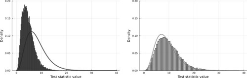
In summary, we find that a chi-squared distribution with G−2 degrees of freedom is inadequate for the HL test when there are binary replicates present in the data. For the generalized HL (GHL) test, it is generally safe to use a chi-squared distribution with G−1 degrees of freedom when the sample size is sufficiently large. These findings are additionally supported by the results of the simulation study of Section 4.

4. Simulation study

4.1. Simulation study design

We compare the performance of the HL and GHL tests by performing an additional simulation study with artificial data. Of particular interest is the rejection rate under the null hypothesis when the tests are applied to moderately large models that are fit to data with clusters or exact replicates in the covariate space. We also consider a power simulation setting to compare the performance of the HL and GHL tests when applied to such data sets. In each simulation setting, 10,000 realizations are produced. All simulations are performed using R.

For the null simulation settings, the true regression model is (3) $\mathbb{E}[Y\mid X=x]=\mathrm{logit}(\alpha +{\beta }_1{x}_1+\cdots +{\beta }_{d-1}{x}_{d-1}),$(3) with d in $\{2,3,\dots ,25\}$. In (3(3) $\mathbb{E}[Y\mid X=x]=\mathrm{logit}(\alpha +{\beta }_1{x}_1+\cdots +{\beta }_{d-1}{x}_{d-1}),$(3) ), α represents the intercept term. To produce replicates in the covariate space, $m\le n$ unique EVPs are drawn randomly from a $(d-1)$-dimensional spherical normal distribution with marginal mean 0 and marginal variance ${\sigma }^2=1$ for each simulation realization. At each EVP, n/m replicate Bernoulli trials are then created, with probabilities determined by (3(3) $\mathbb{E}[Y\mid X=x]=\mathrm{logit}(\alpha +{\beta }_1{x}_1+\cdots +{\beta }_{d-1}{x}_{d-1}),$(3) ). In our simulation study, we fix n = 500 and select $m\in \{50,100,500\}$ so that the number of replicates at each EVP, n/m, is 10, 5, and 1, respectively. We set $\alpha =0.1$ and ${\beta }_1=\cdots ={\beta }_{d-1}=0.535/\sqrt{d-1}$. This results in fitted values that rarely fall outside the interval $[0.1,0.9]$, regardless of the number of parameters in the model, so that the number of expected counts in each group is usually sufficiently large for the use of the Pearson-based test statistics. We also perform some simulations with n = 100, using smaller values of d and m than for n = 500. However, we focus on results for n = 500 because we are then able to increase the number of replicates per EVP, n/m, while still maintaining large enough m so that it is possible to create ten viable groupings.

For the power simulation settings, the true regression model is (4) $\mathbb{E}[Y\mid X=x]=\mathrm{logit}(\alpha +{\beta }_1{x}_1+\cdots +{\beta }_{24}{x}_{24}+{\beta }_{25}{x}_1^2),$(4) and the fitted model is the same as (4(4) $\mathbb{E}[Y\mid X=x]=\mathrm{logit}(\alpha +{\beta }_1{x}_1+\cdots +{\beta }_{24}{x}_{24}+{\beta }_{25}{x}_1^2),$(4) ) except that the quadratic term is not included. Similar to the null settings, we set $\alpha =0.1$, with ${\beta }_1=\cdots ={\beta }_{24}=0.535/\sqrt{24\times 1.0001}$, and vary ${\beta }_{25}\in \{0.0,0.5,1.0,\dots ,2.5\}$ to examine the power of the HL and GHL tests. The coefficients in both the null and power settings were chosen so that the fitted values take on a reasonable range of values and the expected counts in each HL group are usually sufficiently large. The n = 500 data points are generated using the same procedure as for the null simulation settings with m = 50, with an additional perturbation of zero-mean spherical normal noise with variance ${\sigma }_e^2={10}^{-4}$ to each of $x_1,x_2,\dots ,x_{24}$ to avoid issues with forming HL groups when the fitted values are not unique.

4.2. Simulation study results

4.2.1. Null simulations

Figure 2 presents plots of the sample mean and variance of the HL and GHL test statistics against the number of variables in the model, separately for each m. An analogous plot of the estimated type I error rate against the number of variables is also presented. When the HL test is applied to purely binary responses–the m = 500 case–it performs exactly as expected. Its mean, variance, and type I error rate track their respective expectations regardless of model size. However, all three measures show a clear decreasing pattern with increasing model size when replicates are present, with a sharper decrease when the number of replicates per EVP is larger. Because the estimated variance is not always twice the size of the mean, we can infer that the chi-squared approximation to the null distribution of the HL test statistic is not adequate in finite samples for these data structures. Simulation results with a sample size of n = 100 are not displayed but are quite similar.

Figure 2. Null simulation results using n = 500 Bernoulli trials spread across m different unique EVPs. Solid red lines are approximate 95% CIs. Intervals are omitted for the type I error rate plot, but can be approximated by adding and subtracting 0.005 from the estimated rejection rate. Blue horizontal lines indicate means, variances, and type I error rates expected to be seen for the HL and GHL test statistics.

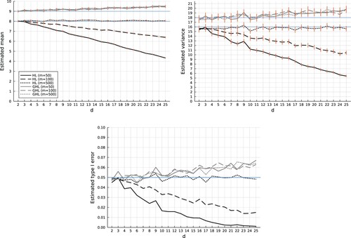
From Figure 2 we also see that the GHL test performs reasonably well in the settings considered. The estimated mean and variance of the test statistic rise slightly above the expected values G−1 = 9 and $2(G-1)=18$, respectively, as the model size grows, but the deviation is not nearly as drastic as for the HL test. Related to this, the GHL test can have an inflated type I error rate, particularly when it is applied to highly complex models. The models considered here are only moderately large, with $d\le min\{n/20,m/2\}$. If one wishes to use the GHL test to assess the quality of fit of models beyond this range, one should be wary of the potential for an inflated type I error rate that may become somewhat larger than we have observed here.

Recall from (1(1) ${\hat{C}}_G\stackrel{d}{\to }{\chi }_{G-d}^2+\sum _{j=1}^d{\lambda }_j{\chi }_{1j}^2,$(1) ) that the asymptotic ${\chi }_{G-2}^2$ distribution for the HL test proposed by [7] is based on a weighted sum of chi-squares that involves a chi-square term with G−d degrees of freedom. We investigated whether maintaining G = 10 while increasing d contributes to the phenomenon we have observed. To this end, we set G = 26 and performed a similar simulation study. However, the adverse behavior of the HL statistic still persists despite this modification.

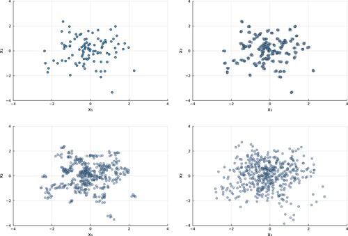
We also investigated the effect of near-replicate clustering in the covariate space. We fixed n and m as in Section 4.1, but added a small amount of random noise with marginal variance ${\sigma }_e^2$ to each replicate within the m sampled vectors. The amount of clustering was controlled by varying ${\sigma }_e^2$, as shown in Figure 3. As expected, increasing ${\sigma }_e^2$, which reduces the clustering of the Bernoulli trials, reduces the severity of the decreasing mean, variance and type I error rate for the HL test statistic. However, the undesirable behavior of the HL test is still evident while ${\sigma }_e^2/{\sigma }^2$ remains small.

Figure 3. Example of clustering in the covariate space with two predictor variables, $X_1$ and $X_2$. Top left to bottom right: ${\sigma }_e^2=0$, 0.001, 0.01, and 0.1, with ${\sigma }^2=1$.

4.2.2. Power simulations

The results of the power simulation study are presented in Table 1. The hypothesis that the undesirable behavior of the HL test under the null also results in reduced power in comparison to the GHL test seems to hold. When the model dimension is large and there is clustering of observations in the covariate space, there is evidence that the power of the regular HL test is considerably lower than that of the GHL test, at least for this particular model deviation.

Table 1. Power simulation results for the HL and GHL tests.

${\beta }_{25}$	HL	GHL
0.0	0.002	0.066
0.5	0.026	0.252
1.0	0.098	0.483
1.5	0.145	0.609
2.0	0.190	0.684
2.5	0.219	0.730

Notes: Entries in the ‘HL’ and ‘GHL’ columns indicate the estimated rejection rates for the two tests.

5. Discussion

The original HL test developed by Hosmer and Lemeshow [7] is a commonly-used test for logistic regression among researchers in biostatistics and the health sciences. Although its performance is well documented [5,6,9], we have identified an issue that does not seem to be well known, other than as speculation in [8]. For moderately large logistic regression models fit to data with binomial count responses, or with binary responses and clusters or exact replicates in the covariate space, the null distribution of the HL test statistic can fail to be adequately represented by a chi-squared distribution in finite samples. Using the original chi-squared distribution with G−2 degrees of freedom can result in a reduced type I error rate, and hence lower power to detect model misspecifications. Based on the results of the simulation study, the GHL test can perform noticeably better in such settings, albeit with a potentially inflated type I error rate.

Similar behavior of the HL test was observed in [13], where the regular HL test was naively generalized to allow for it to be used with Poisson regression models. In their setup, even without the presence of clusters or exact replicates in the covariate space, as the number of model parameters increased for a fixed sample size, the estimated type I error rate decreased. The central matrix in the GHL test statistic, ${\mathrm{\Sigma }}_n$, acts as a form of correction to the HL test statistic by standardizing and by accounting for correlations between the grouped residuals that comprise the quadratic form in both the HL and GHL tests. This is evident from (2(2) $\begin{array}{rl}{\mathrm{\Sigma }}_n& =\frac{1}{n}{G}_n^{\ast }(V_n^{\ast }-V_n^{\ast }{X}^{\ast }(X^{\ast \mathrm{\top }}{V}_n^{\ast }{X}^{\ast }{)}^{-1}{X}^{\ast \mathrm{\top }}{V}_n^{\ast })G_n^{\ast \mathrm{\top }}\\ & =\frac{1}{n}{G}_n^{\ast }{V}_n^{\ast 1/2}(I_n-V_n^{\ast 1/2}{X}^{\ast }(X^{\ast \mathrm{\top }}{V}_n^{\ast }{X}^{\ast }{)}^{-1}{X}^{\ast \mathrm{\top }}{V}_n^{\ast 1/2})V_n^{\ast 1/2}{G}_n^{\ast \mathrm{\top }},\end{array}$(2) ), which shows that ${\mathrm{\Sigma }}_n$ contains the generalized hat matrix subtracted from an identity matrix. To empirically assess the behavior of ${\mathrm{\Sigma }}_n$, we varied ${\sigma }_e^2$ in the setup with replicates and added noise, described at the end of Section 4.2. For large d and moderate n, both fixed, we found that the diagonal elements of ${\mathrm{\Sigma }}_n$ tend to shrink, on average, as ${\sigma }_e^2$ decreases. In contrast, the elements of the HL central matrix remain roughly constant. The GHL statistic seems to adapt to clustering or replicates in X, whereas the HL test statistic does not.

In logistic regression with exact replicates, grouped binary responses can be viewed as binomial responses that might be more influential than sparse binary responses. In this scenario, as d increases for a fixed sample size n, the distribution of the regular HL test statistic diverges from a single chi-squared distribution, suggesting that the standardization offered by the central GHL matrix becomes increasingly important.

The real-life implications of the reduced type I error rate (and hence power) of the regular HL test are that in models with a considerable number of variables, where the data contains clusters or exact replicates, the HL test has limited ability to detect model misspecifications. Failure to detect model misspecification can result in retaining an inadequate model, which is arguably worse than rejecting an adequate model due to an inflated type I error rate. This is particularly true when logistic regression models are used to estimate probabilities from which life-and-death decisions might be made. It also impacts a popular modeling strategy where a simple logistic regression model might be used as a starting approximation for a potentially more complex data structure, expecting to switch to a more complex model if the simpler one is found to be inadequate.

Our advice for choosing between the two GOF tests is displayed as a simple decision tree in Figure 4. The advice should be interpreted for G = 10 groups when d is less than or approximately equal to 25. With very large samples, such as $n\ge 2500$, provided that m is sufficiently large compared to d, it should generally be safe to use the GHL test. Our simulations explored models with $d\le 25$, so some caution should be exercised if the GHL test is to be used with larger models. For small or moderate samples, such as when n = 100 or 500, it is important to identify whether there are clusters or exact replicates in the covariate space. One can compute the number of unique EVPs, m, and compare this number to the sample size, n. For data without exact replicates, clusters in the covariate space can still be detected using one of many existing clustering algorithms, and the average distances between and within clusters can be compared. Informal plots of the $x_i$ projected onto a two- or three-dimensional space can also be used as an aid in this process.

Figure 4. Decision tree offering guidance on how to choose between the two GOF tests with G = 10 groups, based on sample size n, explanatory variable dimension $d\lesssim 25$, and number of unique explanatory variable patterns, m. In each decision, left=no and right=yes.

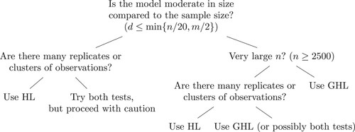
If there is no evidence of clustering or replicates, the HL test should not be disturbed by this phenomenon. On the other hand, if there is a noticeable amount of clustering, and the regression model is not too large, say $d\le min\{n/20,m/2\}$, where m also represents the number of estimated clusters, then one can use the GHL test. In the worst-case scenario with a small sample size, clustering, and a large regression model, one can use both tests as an informal aid in assessing the quality of the fit of the model, recognizing that the GHL test may overstate the lack of fit, while the HL test may understate it. If the two tests agree, then this suggests that the decision is not influenced by the properties of the tests. When they disagree, conclusions should be drawn more tentatively.

Acknowledgments

N.S. additionally acknowledges the support of a Vanier Canada Graduate Scholarship. We thank reviewers of a previous version of this manuscript who made numerous very helpful suggestions that improved the clarity and focus of the paper.

Disclosure statement

No potential conflict of interest was reported by the author(s).

Additional information

Funding

We acknowledge the support of the Natural Sciences and Engineering Research Council of Canada (NSERC), [funding reference number RGPIN-2018-04868].

References

- G. Bertolini, R. D'amico, D. Nardi, A. Tinazzi, and G. Apolone, One model, several results: The paradox of the Hosmer-Lemeshow goodness-of-fit test for the logistic regression model, J. Epidemiol. Biostat. 5 (2000), pp. 251–253.
- C.R. Bilder and T.M. Loughin, Analysis of Categorical Data with R, Chapman and Hall/CRC, Boca Raton, FL, 2014.
- J.D. Canary, L. Blizzard, R.P. Barry, D.W. Hosmer, and S.J. Quinn, Summary goodness-of-fit statistics for binary generalized linear models with noncanonical link functions, Biom. J. 58 (2016), pp. 674–690.
- T. DeHart, H. Tennen, S. Armeli, M. Todd, and G. Affleck, Drinking to regulate negative romantic relationship interactions: The moderating role of self-esteem, J. Exp. Soc. Psychol. 44 (2008), pp. 527–538.
- D.W. Hosmer and N.L. Hjort, Goodness-of-fit processes for logistic regression: Simulation results, Stat. Med. 21 (2002), pp. 2723–2738.
- D.W. Hosmer, T. Hosmer, S. Le Cessie, and S. Lemeshow, A comparison of goodness-of-fit tests for the logistic regression model, Stat. Med. 16 (1997), pp. 965–980.
- D.W. Hosmer and S. Lemeshow, Goodness of fit tests for the multiple logistic regression model, Commun. Stat. Theory Methods 9 (1980), pp. 1043–1069.
- D.W. Hosmer Jr, S. Lemeshow, and R.X. Sturdivant, Applied Logistic Regression, Vol. 398, John Wiley & Sons, Hoboken, NJ, 2013.
- S. Lemeshow and D.W. Hosmer, A review of goodness of fit statistics for use in the development of logistic regression models, Am. J. Epidemiol. 115 (1982), pp. 92–106.
- S. Lemeshow, D. Teres, J.S. Avrunin, and H. Pastides, Predicting the outcome of intensive care unit patients, J. Am. Stat. Assoc. 83 (1988), pp. 348–356.
- D.S. Moore and M.C. Spruill, Unified large-sample theory of general chi-squared statistics for tests of fit, Ann. Stat. 3 (1975), pp. 599–616.
- W. Stute and L.X. Zhu, Model checks for generalized linear models, Scand. J. Stat. 29 (2002), pp. 535–545.
- N. Surjanovic, R. Lockhart, and T.M. Loughin, A generalized Hosmer-Lemeshow goodness-of-fit test for a family of generalized linear models, preprint (2021). Available at arXiv, arXiv:2007.11049.
- A.A. Tsiatis, A note on a goodness-of-fit test for the logistic regression model, Biometrika 67 (1980), pp. 250–251.