Network-based topic structure visualization

Abstract

In the real world, many topics are inter-correlated, making it challenging to investigate their structure and relationships. Understanding the interplay between topics and their relevance can provide valuable insights for researchers, guiding their studies and informing the direction of research. In this paper, we utilize the topic-words distribution, obtained from topic models, as item-response data to model the structure of topics using a latent space item response model. By estimating the latent positions of topics based on their distances toward words, we can capture the underlying topic structure and reveal their relationships. Visualizing the latent positions of topics in Euclidean space allows for an intuitive understanding of their proximity and associations. We interpret relationships among topics by characterizing each topic based on representative words selected using a newly proposed scoring scheme. Additionally, we assess the maturity of topics by tracking their latent positions using different word sets, providing insights into the robustness of topics. To demonstrate the effectiveness of our approach, we analyze the topic composition of COVID-19 studies during the early stage of its emergence using biomedical literature in the PubMed database. The software and data used in this paper are publicly available at https://github.com/jeon9677/gViz.

Keywords:

• Latent space item response model
• topic embedding
• topic structure visualization
• text mining
• network analysis

1. Introduction

Most real-world data rarely consists of independent topics but rather multiple topics that are often inter-correlated. By exploring the relationships and dependencies among topics, researchers can gain a deeper understanding of the underlying structure and dynamics of their research domain. This understanding can help identify emerging trends, uncover research gaps, and highlight areas of high importance or potential impact. It can help researchers be knowledgeable of research areas that are emerging and/or significant to the field and allow them to put their efforts into important ones. There have been attempts to model correlated structure among topics by modeling the correlated structure within the topic model or combining the topic model with statistical models. For instance, Blei and Lafferty [3] regarded the topic of correlation as a structure of heterogeneity. To capture the heterogeneity of topics, they suggested the correlated topic model (CTM), which models topic proportions to exhibit correlation through the logistic normal distribution within Latent Dirichlet Allocation (LDA). Rusch et al. [11] combined LDA with decision trees to interpret the topic relationships from Afghanistan war logs. It classified the topics using tree structures, which helped to understand the different circumstances in the Afghanistan war. However, these approaches do not directly allow us to investigate the degree of correlation and closeness among topics. To address this, Sievert and Shirley [13] attempted to quantify the relationships and proximity between topics by calculating the distances between topics. Specifically, they used multi-dimensional scaling (MDS) to embed the topics on a metric space based on a distance matrix calculated from the output of a topic model (LDA). However, MDS requires specification of similarity and dissimilarity measures to construct the distance matrix and the results can be significantly affected by the choice of measures in spite of their ad hocness. In practice, it is often difficult to determine the appropriate measures for calculating and defining distances between topics. Hence, it is beneficial to have a unified approach to estimate the structure of topics, which allows us to avoid such ad hoc choices and guarantee more consistent results. One of the statistical methods for handling correlated structures is network analysis. Specifically, the network model estimates the relationships among nodes based on their dependency structure. Moreover, it can provide global and local representation of nodes at the same time. In this context, Mei et al. [9] tried to identify topical communities by combining a topic model with a social network approach. Specifically, it estimated topic relationships given the known network structure and tried to separate out topics based on connectivity among them. However, in this approach, the network information needs to be provided to construct and visualize the topic network, which is not a trivial task in practice.

To address this, we propose an alternative approach to examine the structure of topics using the information from the output of topic models. Specifically, our approach leverages a latent space network model, which estimates the relationships among nodes by estimating topics' latent positions. The latent positions can then be used to quantify the relationships among nodes, i.e. the distances between topics. In our study, we treat the output of the topic-words distribution as a topic-words matrix $\mathbf{X}$, which can be seen as an item-response data [5] with an inter-correlated structure. Using this matrix, we simultaneously estimate the relationship between topics and words, which yields the latent position of topics. When two topics share similar word meanings, their latent positions are located close to each other, making it easier to understand relationships between topics based on their associated words. Furthermore, when topics share common words, their latent positions tend to be located near the origin. Conversely, topics that incorporate more distinctive and exclusive words compared to other topics tend to be positioned farther away from the origin. This behavior elucidates the relationship between the words associated with topics and their respective positions in the latent space. This also enables us to visualize the structure of topics using the estimated latent positions.

In this approach, we interpret the relationships among topics by characterizing topics based on their representative words. If two topics are closely located in the latent positions, they might deliver similar meanings in documents. To make the process of selecting meaningful words within the topics more efficient and objective, it is desirable to have a score calculated based on the information provided by our analytical framework. Previously Airoldi and Bischof [1] evaluated the topics using the novel score called FREX, which quantifies words' closeness within the topic based on the word frequency and exclusivity. Here, ${\mathit{FREX}}_{\mathit{i}\mathit{,}\mathit{j}}$ reflects how word j is exclusively close to topic i compared to other topics. However, relying solely on the frequency of words in documents is not enough to identify keywords within topics that reflect the association among topics. To address this, here we propose a score that takes into account both (i) the probability of words belonging to each topic based on the frequency of associated words using the topic model; and (ii) how closely words are exclusively related to each topic by considering the relevance between topics using the network model. By putting these two pieces of information together, our analytical framework can pick up information about relativeness and exclusivity.

It is also important to acknowledge the fact that topics also vary in the sense of how mature it is and whether they are common or specific. We can evaluate this by checking whether the latent positions of topics are robust to different word sizes. This is based on the rationale that mature topics and/or those consisting of common words might remain similar and stable upon changes in word sets, compared to emerging or specific topics. Hence, to understand the changes in the latent positions of topics, we track the latent positions of topics by differing word sets. To select word sets of different sizes, we used two criteria to select informative words: high coefficient variation and high maximum probability from topic-words distribution. First, words with large variations in probabilities among topics are expected to be more important because if a word has low variation across topics, it is likely that the word does not represent any topic specifically. We used the coefficient of variation to characterize words' dispersion among topics. Second, a meaningful word should have a high probability in at least one topic. Even when a word has high variation among topics, if that word has only low probabilities across topics, it might not be informative to differentiate topics.

The rest of this article is organized as follows. In Section 2, we introduce our dataset and the Gaussian version of the latent space item response model [8], which estimates latent positions of topics based on their latent distances between words. In addition, we introduce our scoring scheme that helps to select representative words from each topic to enhance the understanding of the topic structure. In Section 3, we apply our approach to the COVID-19 literature to evaluate and demonstrate the usefulness of our approach. In Section 4, we summarize our topic structure visualization with a conclusion.

2. Methodology

2.1. Data

Since the emergence of the worldwide pandemic of COVID-19, relevant research has been published at a dazzling pace, which yields an abundant amount of big data in biomedical literature. Due to the high volume of relevant literature, it is practically impossible to follow up the research manually. Furthermore, in the early stages of research when a specific topic has not yet been established, many studies are likely to be connected to each other. Therefore, by examining which topics are being discussed together, we can more easily understand the research direction of COVID-19. For instance, if some researchers want to investigate a specific topic, say ‘COVID-19 symptoms’, we want to answer the questions like the following: (1) Which set of words are associated with ‘COVID-19 symptoms’? (2) Are there any other topics related to ‘COVID-19 symptoms’, which can be used for extending and elaborating research? (3) Is ‘COVID-19 symptoms’ a common or specific topic?

To model the COVID-19 literature, we downloaded the COVID-19 articles published from the PubMed database (https://pubmed.ncbi.nlm.nih.gov) with a time-frame between December 1st, 2019, and August 3rd, 2020, coinciding with the date of the WHO's designation of COVID-19 as a pandemic. We collected articles whose titles contained “coronavirus2”, “covid-19” or “SARS-CoV-2”, which resulted in a total of 35,585 articles. Since COVID-19 was a worldwide pandemic that spread at an unprecedented rate, some articles that examine COVID-19 have been published with only an abstract. After eliminating articles without abstracts (i.e. only titles or abstract keywords), our final text data contained a total of 15,015 abstracts.

Based on the abstracts, we constructed the corpus using the abstract keywords that concisely captured the messages delivered by the paper. To enrich the corpus, we further used the word2vec approach [10] to train against relationships between nouns from the abstract and the abstract keywords. Specifically, word2vec extracted nouns from abstracts, which were embedded near the abstract keywords, and added those selected words to the corpus. Using the trained word2vec network with 256 dimensions, we selected ten words from the abstract nouns that were near each abstract keyword. We provide the details of our training strategy for the word2vec network in the Supplemental Materials (see Appendix A). The corpus construction resulted in 9,643 words from 15,015 documents. We further filtered out noise words, including single alphabets, numbers, and other words that are not meaningful, e.g. ‘p.001’, ‘p.05’, ‘n1427’, ‘l.’, and ‘ie’. Finally, to obtain more meaningful topics, we removed common words like ‘data’, ‘analysis’, ‘fact’, and ‘disease’. We provide the full list of filtered keywords in the Supplemental Materials (see Appendix B).

To obtain the topic-words matrix, we implemented the topic modeling. Since the abstracts of the COVID-19 literature are categorized as short text, conventional topic models including LDA often suffer from poor performance due to the sparsity problem. Yan et al. [14] made important progress in the modeling of short text data, the so-called Biterm Topic Model (BTM). Unlike the LDA, BTM replaced words with bi-terms, where a bi-term is defined as a set of two words occurring in the same document. This approach attempted to compensate for the lack of words in a short text by pairing two words, thereby creating more words in the document. This is based on the observation that if two words are mentioned together, they are more likely to belong to the same topic. Using the BTM, we were able to obtain a topic-words distribution, which is essentially a matrix of topics and their associated words. In the following section, we introduce how we utilize the topic-words matrix as an input for the latent space item response model to estimate topics' interactions based on their association with words.

2.2. Estimating topic relationships using latent space item response model

Hoff et al. [6] proposed the latent space model, which expresses a relationship between actors of a network in an unobserved “social space”, so-called latent space. Inspired by Hoff et al. [6], Jeon et al. [8] proposed the latent space item response model (LSIRM) that viewed item response as a bipartite network and estimated the relationship between respondents and items using the latent space. In order to achieve our objective of estimating the topic structure and visualizing their relationships, we utilized the concept of latent positions. These latent positions allow us to estimate the relevance of topics based on the distances between topics and associated words. By measuring the closeness between topics in terms of their latent positions, we can intuitively represent their distances.

However, the original LSIRM proposed by Jeon et al. [8] is not directly applicable here because it was designed for a binary item response dataset, where each cell in the item response data is binary-valued (0 or 1). On the contrary, the output of BTM is in the form of probabilities, indicating how likely each word belongs to each topic. Furthermore, given the large number of words, there are instances where the probability is near 0. To address these issues, we employ logit transformation to prepare the input data for LSIRM. This transformation yields continuous values ranging from $(-\mathrm{\infty },+\mathrm{\infty })$ and effectively amplifies differences among probabilities. Let $\mathbf{X}$ be the logit-transformed input where each item represents a topic i and each respondent corresponds to word j for $i=1,\dots ,P$ and $j=1,\dots ,N$. Here ${\mathbf{v}}_{\mathbf{i}}\in {\mathbb{R}}^{\mathbf{d}}$ and ${\mathbf{u}}_{\mathbf{j}}\in {\mathbb{R}}^{\mathbf{d}}$ be the d-dimensional latent positions. We apply logit-transformed $\mathbf{X}$ to the continuous version of LSIRM, which can be written as $\begin{array}{rl}{x}_{i,j}\mid \mathbf{\Theta }& ={\beta }_i+{\theta }_j-||{\mathbf{v}}_i-{\mathbf{u}}_j||+{ϵ}_{i,j},\\ {ϵ}_{i,j}& \sim \text{N}(0,{\sigma }^2),\end{array}$ where $x_{i,j}$ indicates the logit-transformed probability that word j belongs to topic i. Here, ${\beta }_i$ and ${\theta }_j$ represent the intercepts for topic i and word j, respectively, and $||{\mathbf{v}}_i-{\mathbf{u}}_j||$ represents the Euclidean distance between latent positions of word j and topic i. We estimate the relevance between topics by measuring the distances between topics. Note that the distances between topics are measured based on their relationships with words. Specifically, if two topics share similar word sets, we consider them to have a close relationship and estimate their relationship accordingly. In contrast to the original LSIRM, which used a logit link function to handle the binary data, here we assume linearity between $x_{i,j}$ and the attribute part with the relevance part. We added an error term ${ϵ}_{i,j}\sim N(0,{\sigma }^2)$ to satisfy the normality equation. Given the model described above, we use Bayesian inference to estimate parameters in the Gaussian version of LSIRM. We use the notation $\mathbf{\Theta }=\{\mathit{\beta }=\{{\beta }_i{\}}_{i=1}^P,\mathit{\theta }=\{{\theta }_j{\}}_{j=1}^N,\mathbf{V}\mathbf{=}\{{\mathbf{v}}_{\mathbf{i}}\}{\}}_{\mathbf{i}\mathbf{=}\mathbf{1}}^{\mathbf{P}}\mathbf{,}\mathbf{U}\mathbf{=}\{{\mathbf{u}}_{\mathbf{j}}{\}}_{\mathbf{j}\mathbf{=}\mathbf{1}}^{\mathbf{N}}\mathbf{,}{\sigma }_{\theta }^{\mathbf{2}}\}$ for parameter set of our model. We specify prior distributions for the parameters as follows: $\begin{array}{rl}{\beta }_i& \sim \mathrm{N}(0,1),\\ {\theta }_j|{\sigma }_{\theta }^2& \sim \mathrm{N}(0,{\sigma }_{\theta }^2),{\sigma }^2>0\\ {\sigma }^2& \sim \mathrm{Inv}-\mathrm{Gamma}(a,b),a_{>}0,b>0\\ {\sigma }_{\theta }^2& \sim \mathrm{Inv}-\mathrm{Gamma}(a_{\sigma },b_{\sigma }),a_{\sigma }>0,b_{\sigma }>0\\ {\mathbf{u}}_{\mathbf{j}}& \sim {\mathrm{MVN}}_d({\mathbf{0}\mathbf{,}\mathbf{I}}_d)\\ {\mathbf{v}}_{\mathbf{i}}& \sim {\mathrm{MVN}}_d({\mathbf{0}\mathbf{,}\mathbf{I}}_d),\end{array}$ where $\mathbf{0}$ is a length-d vector of zeros and ${\mathbf{I}}_d$ is the $d\times d$ identify matrix. We treat ${\beta }_i$ as a fixed effect and ${\theta }_j$ as a random effect in order to account for the variability among words. By including a random effect, the model acknowledges that different words may exhibit unique patterns and behaviors toward specific topics. The posterior distribution of LSIRM is $\pi (\mathbf{\Theta },{\sigma }^2|\mathbf{X}\mathbf{)}\propto \prod _{\mathbf{j}}\prod _{\mathbf{i}}\mathbb{P}\left({\mathbf{x}}_{\mathbf{i}\mathbf{,}\mathbf{j}}\mathbf{|}\mathbf{\Theta }\right)\prod _{\mathbf{j}}\pi \mathbf{(}{\mathit{\theta }}_{\mathbf{j}}\mathbf{|}{\sigma }_{\theta }^{\mathbf{2}}\mathbf{)}\pi \mathbf{(}{\sigma }_{\theta }^{\mathbf{2}}\mathbf{)}\prod _{\mathbf{i}}\pi \mathbf{(}{\mathit{\beta }}_{\mathbf{i}}\mathbf{)}\prod _{\mathbf{j}}\pi \mathbf{(}{\mathbf{u}}_{\mathbf{j}}\mathbf{)}\prod _{\mathbf{i}}\pi \mathbf{(}{\mathbf{v}}_{\mathbf{i}}\mathbf{)}\pi \mathbf{(}{\sigma }^{\mathbf{2}}\mathbf{)}$ and we use Markov Chain Montel Carlo (MCMC) to estimate the parameters of LSIRM. We provide the full inference of MCMC steps in the Appendix D of the Supplemental Materials. In this way, we can obtain latent positions of ${\mathbf{u}}_j$ and ${\mathbf{v}}_i$ on the ${\mathbf{R}}^d$. Since we are interested in constructing the topic network, we utilize ${\mathbf{v}}_i,i=1,\dots ,P$ and make it as matrices of $\mathbf{A}\in {\mathbf{R}}^{P\times d}$ where row indicates P number of topics and column indicates d number of dimension of coordinates.

The latent positions of topics are assumed to follow a standard normal distribution. As a result, there is a tendency for these latent positions to spread out from the origin. Specifically, when topics share common words, their latent positions tend to be located near the origin, indicating their similarity. On the other hand, topics with more distinctive and exclusive words compared to other topics tend to be positioned farther away from the origin, indicating their uniqueness. This behavior illustrates the relationship between the words associated with topics and their corresponding positions in the latent space. Therefore, latent positions of topics not only enable us to visualize the dependency structure of topics but also help us understand the topic structure through their spreading tendency.

Here we further improve the interpretation of relationships among topics by tracing how topics' latent positions evolve with increasing word size. Let ${\mathbf{X}}_k$ denote the topic-words matrix where the subscript k indicates the $k\mathrm{\%}$ inclusion probability of words. Therefore, as the value of $k\mathrm{\%}$ increases, more words are included in the topic-words matrix ${\mathbf{X}}_k$. After proceeding with the LSIRM model with various sets of matrices ${\mathbf{X}}_k$, we can obtain matrices of ${\mathbf{A}}_k$, composed of coordinates of each topic. Since the distances between pairs of words and topics, which are crucial for inferring latent positions, can be subject to variations due to rotation, translation, and reflection, multiple possible realizations of latent positions can exist. These variations in the likelihood function necessitate careful consideration to ensure accurate estimation and inference [6,12].

To tackle this invariance property for determining latent positions, we implement Procrustes matching [4] as post-processing two times: (1) within-matrix Procrustes matching and (2) between-matrix Procrustes matching. First, we implement so-called within-matrix matching within the MCMC samples for each topic's latent positions generated from LSIRM. Second, we implemented so-called between-matrix matching for the estimated matrices to locate topics in the same quadrant. To align the latent positions of topics, we need to set up the baseline matrix, denoted as ${\mathbf{A}}_{max}$, which maximizes the dependency structure among topics. To measure the degree of dependency structure, we take the average of the distances of topics' latent positions from the origin. The longer distance of latent positions from the origin implies a stronger dependency on the network. It helps nicely show the change of topics' latent positions because those rotated positions ${\mathbf{A}}_k$ from each matrix ${\mathbf{X}}_k$ are based on the most stretched-out network from the origin. As a result, we can obtain the re-positioned matrices ${\mathbf{A}}_k^{\ast }$, which still maintain the dependency structure among topics but are located in the same quadrant.

With the oblique rotation, the interpretation of axes can be further improved and topics can be categorized based on these axes. For this purpose, we applied the oblim rotation [7] to the estimated topic position matrix ${\mathbf{A}}_k^{\ast }$, using the R package GPAroation [2]. We denote the rotated topic position metric by ${\mathbf{B}}_k$. To interpret the trajectory plot showing traces of topics' latent positions, we extracted the rotation information matrix ($\mathbf{R}$) resulting from an oblique rotation as the baseline matrix ${\mathbf{B}}_{\mathrm{base}}$. Then, we multiplied each matrix (${\mathbf{B}}_k$) by the rotation matrix ($\mathbf{R}$) to plot the topics' latent positions.

2.3. Scoring the words relation to topics

By combining the idea from Airoldi and Bischof [1] with the relevance information among topics in our problem, here we propose the score $s_{i,j}$ which measures the exclusiveness of word j in the topic i. We define score $s_{i,j}$ as (1) $\begin{array}{rl}{s}_{i,j}& =\left(\frac{w_1}{2-{\mathrm{ECDF}}_{{\mathit{\delta }}_{.,j}}({\delta }_{i,j})}\right)+\left(\frac{w_2}{2-{\mathrm{ECDF}}_{{\mathit{\delta }}_{i,.}}({\delta }_{i,j})}\right)\\ & +\left(\frac{w_3}{1+{\mathrm{ECDF}}_{{\mathit{\gamma }}_{.,j}}({\gamma }_{i,j})}\right)+\left(\frac{w_4}{1+{\mathrm{ECDF}}_{{\mathit{\gamma }}_{i,.}}({\gamma }_{i,j})}\right),\end{array}$(1) where $w_i$, i = 1, 2, 3, 4, represents the weights for exclusivity, and $\mathrm{ECDF}$ denotes the empirical CDF function. To provide an intuitive interpretation of the score value, we normalize the score to range between 0 and 1 by ensuring that $\sum _{i=1}^4{w}_i=1$. Without prior knowledge, one can assign equal weight to each term in the score by setting $w_1=w_2=w_3=w_4=0.25$. However, when dealing with a corpus that includes redundant words, the probability derived from topic models might reduce the exclusivity of word j within topic i. In such cases, incorporating distances between latent positions may offer a more suitable measure of the exclusiveness of word j in topic i. Since our approach focuses on selecting meaningful words and estimating interactions between word j and topic i, assigning higher values to $w_3$ and $w_4$ could be beneficial in such scenarios. Here, ${\delta }_{i,j}$ denotes the probability of word j belonging to topic i given by BTM, and ${\gamma }_{i,j}$ is the distance between the latent position of word j and topic i estimated by LSIRM. The higher value of ${\delta }_{i,j}$ indicates the closer relationship between word j and topic i, and the smaller value of ${\gamma }_{i,j}$ indicates the shorter distance between word j and topic i. To make the meaning of the shorter distance and the higher probability consistent as both contribute to the higher scores, first, we subtracted ${\mathrm{ECDF}}_{{\mathit{\delta }}_{.,j}}({\delta }_{i,j})$ and ${\mathrm{ECDF}}_{{\mathit{\delta }}_{i,.}}({\delta }_{i,j})$ from 2. Note that here we use 2 to avoid the zero in the denominator. For example, if ${\delta }_{i,j}$ has a higher probability within the topic i and between the other topics and word j, then both $2-{\mathrm{ECDF}}_{{\mathit{\delta }}_{.,j}({\delta }_{i,j})}$ and $2-{\mathrm{ECDF}}_{{\mathit{\delta }}_{i,.}({\delta }_{i,j})}$ will have smaller values. This means that the word j is distinctive enough to represent the meaning of topic i. Second, if the latent distance between word j and topic i has the shorter distance within topic i than between the other topics and word j, then both $1+{\mathrm{ECDF}}_{{\mathit{\gamma }}_{.,j}({\gamma }_{i,j})}$ and $1+{\mathrm{ECDF}}_{{\mathit{\gamma }}_{i,.}({\gamma }_{i,j})}$ have the smaller values contributing to a higher score $s_{i,j}$. Here we added 1 to each denominator term, preventing the denominator from becoming zero. Based on $s_{i,j}$, we can determine whether the word j and the topic i are close enough to be mentioned in the same document. By collecting the high-score words, we can characterize the topics.

3. Application

3.1. Topic-words matrix of COVID-19 biomedical literature using BTM

To implement BTM, we set the topic number to 20. For the hyper-parameters, we assigned $\alpha =3$ and $\beta =0.01$. Since our main goal is to estimate the topic structure, we empirically searched and determined the hyper-parameters of BTM. We explain the details of the modeling of the topic model in the Supplemental Materials (see Appendix C). The posterior distribution of the topic-words was estimated using the Gibbs sampler. Specifically, we generated samples with 50,000 iterations after the 20,000 burn-in iterations and then implemented thinning for every ${100}^{\mathrm{th}}$ iteration.

In each topic-words distribution obtained from BTM, words with high probabilities characterize the topic. Since the topic-words distribution contains all the word sets from the corpus, using all word sets can lead to redundancy. To confirm this, we draw a histogram of log-transformed probabilities and it shows bimodal topic-words distributions. This pattern indicates that some words had low probabilities of belonging to a specific topic, whereas the mode in the center corresponds to the words that have probabilities high enough to characterize the meaning of the topic. Therefore, it might be more desirable to estimate topic structure using only the words corresponding to the mode in the center rather than all the words. On the other hand, our exploratory analysis indicated that more than 1000 words are needed to represent topics properly. Based on this rationale, we decided to use at least 1000 words to estimate the positions of topics in the latent space based on the positions of words. Given the selected minimum number of words, we extracted meaningful words that can characterize topics based on the coefficient of variation and maximum probability.

Given the coefficient of variation and maximum probability, we obtained multiple matrices corresponding to the top 60% to 40% of words determined based on the two criteria. The numbers of words corresponding to the ${60}^{\mathrm{th}}$ and ${40}^{\mathrm{th}}$ percentiles were 2,648 and 1,095, respectively. We applied a logit transformation to the values in these matrices, which originally ranged between 0 and 1, to convert them into continuous values ranging from $-\mathrm{\infty }$ to ∞. Therefore, we used 21 sets of logit-transformed matrices, ${\mathbf{X}}_k(k=40\mathrm{\%},\dots ,60\mathrm{\%})$, as the LSIRM input data, where their dimensions were ranged from $2,648\times 20$ to $1095\times 20$. In this way, we obtained the 21 sets of matrices ${\mathbf{X}}_k$ and we considered 20 topics for all the matrix sets.

3.2. LSIRM for topic-words matrix

To run the LSIRM, MCMC was implemented to estimate topics' latent positions $\mathbf{V}\mathbf{=}\{{\mathbf{v}}_{\mathbf{i}}\}$ where $i=1,\dots ,20$. The MCMC ran 55,000 iterations, and the first 5000 iterations were discarded as burned-in processes. Then, from the remaining 50,000 iterations, we collected 10,000 samples using a thinning of 5. To visualize relationships among topics, we used two-dimensional Euclidean space. Additionally, we set 0.28 for $\mathit{\beta }$ jumping rule, 1 for $\mathit{\theta }$ jumping rule, and 0.06 for ${\mathbf{u}}_j$ and ${\mathbf{v}}_i$ jumping rules. Here, we fixed prior $\mathit{\beta }\sim N(0,1)$. On the other hand, we set $a_{\sigma }=b_{\sigma }=0.001$ and a = b = 0.001 for non-informative prior for ${\sigma }_{\theta }^2$ and ${\sigma }^2$.

LSIRM takes each matrix ${\mathbf{X}}_k$ as input and provides the ${\mathbf{A}}_k$ matrix as output after the Procrustes-matching within the model. Since we calculated topics' distance on the 2-dimensional Euclidean space, ${\mathbf{A}}_k$ is of dimension $20\times 2$. We visualized the topic structure using the baseline matrix ${\mathbf{A}}_{max}$ so that we can compare topics' latent positions without having identifiable issues from the invariance property. From ${\mathbf{A}}_k$, we calculated the distance between the origin and each topic's coordinates. The closer distance of a topic position from the origin indicates a weaker dependency on other topics. In our interrogation of ${\mathbf{A}}_k$, we found that the dependency structure among topics starts to be built up from ${\mathbf{A}}_{47\mathrm{\%}}$. There are two possibilities that can lead to low dependency. First, it is possible that a small number of words could distinguish the characteristics of their topics from the other topics. Second, it is possible that most of the words were commonly shared with other topics. We provide the distance plot of ${\mathbf{A}}_k$ in the Supplemental Materials (see Appendix E). Based on this rationale, we chose ${\mathbf{A}}_{47\mathrm{\%}}$ as the baseline matrix ${\mathbf{A}}_{max}$. With this baseline matrix ${\mathbf{A}}_{47\mathrm{\%}}$, we implemented the Procrustes matching to align the direction of the topic's latent positions from each matrix ${\mathbf{A}}_k$. Using this process, we could obtain the ${\mathbf{A}}_k^{\ast }$ matrix matched to the baseline matrix ${\mathbf{A}}_{47\mathrm{\%}}$. We named the identified topics based on top-ranking words using the ${\mathbf{A}}_{47\mathrm{\%}}$ matrix because the baseline matrix ${\mathbf{A}}_{47\mathrm{\%}}$ has the most substantial dependency structure. We applied oblimin rotation to the estimated topic position matrix ${\mathbf{A}}_{k\mathrm{\%}}^{\ast }$ using the R package GPArotation[2], and obtained matrix ${\mathbf{B}}_k$ $k=40\mathrm{\%},\dots ,60\mathrm{\%}$ with the rotation matrix $\mathbf{R}$. By rotating the original latent space, we could obtain more interpretable axes for the identified latent space (e.g. determining the meaning of a topic's transition based on the X-axis or Y-axis).

3.3. Words selection for each topic based on the score

We calculated the score $s_{i,j}$ for each word j with topic i based on each ${\mathbf{B}}_{\mathbf{k}}$ for $k=40\mathrm{\%},\dots ,60\mathrm{\%}$. In our application, we assigned equal weight to each term, by setting $w_1=w_2=w_3=w_4=0.25$. This choice reflects a balanced consideration of both the probability from topic models and the distances between latent positions in determining the exclusivity of words within topics. The resulting score and affinity plot for each topic from ${\mathbf{B}}_{47\mathrm{\%}}$ can be found in Appendix F of the Supplemental Materials. To further explore the impact of different weight assignments on the exclusivity score and affinity plot, we provide additional visualizations for each topic using varying weights in Appendix G of the Supplemental Materials. Figure 1 shows the two different scenarios of the plot of $s_{i,j}$ and affinity ($\exp (-{\gamma }_{i,j})$) in ${\mathbf{B}}_{47\mathrm{\%}}$; one with a high score and higher affinity, and the other with a high score but lower affinity. Figure 1(a) shows the estimated latent positions of topics obtained from ${\mathbf{B}}_{47\mathrm{\%}}$. We can see that topics 2, 7, 13, 14, 19, and 20 are located around the origin, indicating their general nature and similarity in terms of their word composition. These common topics share many words in common with other nearby topics, making it challenging to discern their unique characteristics solely based on word probabilities (Figure 1(b)). On the other hand, the remaining topics are positioned away from the origin, indicating that they have distinctive characteristics compared to other topics (Figure 1(c)). For these topics, it is important to understand their direction and identify which topics are closely related. We extracted the top 20% of words with high values in score to interpret each topic and we collected the meaningful words that commonly appear at the top of the list among every portion of words set ${\mathbf{B}}_k,k=40\mathrm{\%},\dots ,60\mathrm{\%}$. Table 1 shows the interpretation of each topic made based on the selected words with its top score words.

Figure 1. If topics are located in the center in latent position (a), two distinct subgroups are observed in the score and affinity plot (b). Otherwise, such subgroup patterns are not observed in the score and affinity plot (c). In (b) and (c), the orange color (id of 1) indicates the top 20% of words of high score words while the green color (id of 0) indicates the remaining words. (a) Topics' latent positions of ${\mathbf{B}}_{47\mathrm{\%}}$. (b) The score and affinity plot of Topic 19 in ${\mathbf{B}}_{47\mathrm{\%}}$ and (c) The score and affinity plot of Topic 3 in ${\mathbf{B}}_{47\mathrm{\%}}$.

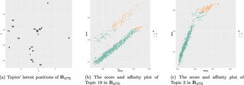
Table 1. Interpretation of the topic based on ${\mathbf{A}}_{47\mathrm{\%}}^{\ast }$ matrix.

Topic	Name	Top score words
1	Lung Scan (Imaging)	subpleural	crazy paving	bronchogram
		(0.963)	(0.957)	(0.950)
2	Compound and Drug	Protein Data Bank	papain-like	intermolecular
		(0.938)	(0.936)	(0.934)
3	Microbiome	${\mathrm{DHA}}^{\ast }$	biofilm	vancomycin-resistant
		(0.968)	(0.968)	(0.967)
4	Treatment of Other Diseases	sarcoma	arthroplasty	neoadjuvant
		(0.948)	(0.944)	(0.943)
5	Cardiovascular (Symptom)	vein	antithrombotic	${\mathrm{VTE}}^{\ast }$
		(0.906)	(0.899)	(0.898)
6	Molecular-level Response to Infection	${\mathrm{NLRP}3}^{\ast }$	metalloproteinase	upregulation
		(0.929)	(0.927)	(0.926)
7	COVID-19 Risk Prediction Markers	alanin	${\mathrm{BUN}}^{\ast }$	prealbumin
		(0.976)	(0.972)	(0.969)
8	Literature Review	Prospero DB	Wanfang DB	meta-analys
		(0.967)	(0.966)	(0.944)
9	Symptom and Comorbidity	petechiae	guillain-barre syndrome	ageusia
		(0.958)	(0.955)	(0.952)
10	Cardiovascular	infarction	thromboprophylaxis	${\mathrm{VTE}}^{\ast }$
		(0.912)	(0.909)	(0.909)
11	Social Impact	classroom	pedagogy	zoom
		(0.925)	(0.911)	(0.906)
12	Financial and Economical Impact	macroeconomics	monetary	profit
		(0.929)	(0.928)	(0.928)
13	Statistical Modeling	Weibull	least-square	${\mathrm{MAE}}^{\ast }$
		(0.984)	(0.975)	(0.966)
14	COVID-19 Test	${\mathrm{LFIAs}}^{\ast }$	transcription-${\mathrm{PCR}}^{\ast }$	Wantai
		(0.979)	(0.974)	(0.972)
15	Mental Issues	anxious	${\mathrm{PTSD}}^{\ast }$	post-traumatic
		(0.942)	(0.940)	(0.935)
16	Lung Scan	procalcitonin	ground-glass	opacity
		(0.924)	(0.922)	(0.916)
17	Treatment of COVID-19	reintubation	multi-centric	Hydroxychloroquine
		(0.943)	(0.943)	(0.937)
18	Respiration	laryngoscope	facepiece	supraglottic
		(0.978)	(0.978)	(0.975)
19	Prevention of COVID-19	alcohol-based	decontamination	rub
		(0.944)	(0.941)	(0.919)
20	Immunology and Virus	${\mathrm{MHC}}^{\ast }$	multi-epitope	immunodominant
		(0.976)	(0.975)	(0.973)

Note: The abbreviation is marked by an asterisk and a more detailed interpretation can be found in the Supplemental Materials (see Appendix H).

3.4. COVID-19 topic structure visualization

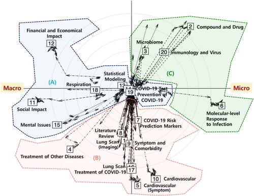
We interrogated what kinds of topics have been extensively studied in the biomedical literature on COVID-19. In addition, we also studied how those topics were related to each other, based on their closeness in the sense of latent positions. We also partially clustered the topics based on their relationships using the quadrants. This allows us to check which studies about COVID-19 are relevant to each other and could be integrated. Figure 2 displays the trajectory plot and it shows how topics were positioned on the latent space and how these topics make the transition across word sets of different sizes. Here the direction of arrows refers to how topics' coordinates changed as a function of the number of words, where each arrow moved from ${\mathbf{B}}_{60\mathrm{\%}}$ to ${\mathbf{B}}_{40\mathrm{\%}}$ as the number of words decreased.

Figure 2. Topic architecture visualization of COVID-19 literature with three topic clusters (A)–(C). The arrow indicates the direction of latent positions by increasing the word size. (A) COVID-19 and its impacts on different areas. (B) Symptoms and treatment of COVID-19 and relevant studies. (C) Molecular studies associated with the COVID-19 infection.

It is important to note that we named the topics based on their top-scoring words and observed that topics with similar meanings tend to have similar directions, with their latent positions located closely together. For example, the twentieth topic is related to immunology and viruses, which includes words like ‘major histocompatibility complex(MHC)(0.976)’, ‘multi-epitope(0.975)’, and ‘immunodominant(0.973)’, all of which are associated with the antigen peptide recognition and relevant immune response. The second topic discusses compounds and drugs, which include words like ‘protein data bank(PDB)(0.938)’ and ‘Papain-like protease(0.936)’ (which is an essential coronavirus enzyme), and ‘inter-molecular(0.934)’. The third topic is related to microbiome in the context of COVID-19 and includes words such as ‘docosahexaenoic(DHA)(0.968)’, ‘biofilm(0.968)’, and ‘vancomycin-resistant(0.967)’ (which is related to antibiotic-resistance). The latent positions of these three topics are closely located, which is sensible given the interaction between the immune system and viral infections, and the role of microbiota as a key component of this interaction.

Furthermore, the latent positions of the seventh, ninth, and seventeenth topics align in a coherent trajectory, reflecting a continuum from risk assessment to treatment in the context of COVID-19. The seventeenth topic is about COVID-19 risk prediction markers and includes words like ‘alanin(0.976)’, ‘Blood Urea Nitrogen(BUN)(0.972)’, and ‘prealbumin(0.969)’. This topic provides insight into medical indicators crucial for assessing the risk associated with the disease. The ninth topic describes COVID-19 symptoms and comorbidity such as ‘petechiae(0.958)’, ‘Guillain-Barre syndrome(0.955)’ (the condition that the immune system attacks the nerves), and ‘aguesia(0.952)’ (loss of taste experienced by COVID-19 patients). The seventeenth topic is about the treatment of COVID-19 and includes words like ‘reintubation(0.943)’ (a common complication in critically ill patients requiring mechanical ventilation), ‘multi-centric(0.943)’, and ‘hydroxychloroquine(HCQ)(0.937)’, which are considered to be the interventions and strategies employed to manage and mitigate the effects of the disease. Although there are limitations to directly validating the top-scoring words, we can indirectly gauge the significance of our topic naming by examining the proximity of latent positions, which correlates with the context and coherence of each topic's meaning.

According to Figure 2, we observed three distinct patterns. The first pattern consists of topics that have common words shared among them, while the second and third patterns consist of topics that have their own distinct words but are different in recursion. First, the topics ‘Statistical Modeling’, ‘COVID-19 Test’, and ‘Prevention of COVID-19’ (Topics 13, 14, and 19, respectively) were located in the center of the plot (the former group). This indicates that no matter how many words were used to estimate the topics' latent positions, those topics remained as general topics and shared many words with other topics. Second, the topics ‘Financial and Economical Impact’, ‘Social Impact’, ‘Cardiovascular’, and ‘Molecular-level Response to Infection’ (Topics 12, 11, 10, and 6, respectively) were located away from the center of the plot (the latter group), which implies their dependency structures with other topics. These topics usually stay on the boundary of the plot regardless of the number of words because they mainly consist of unique words. Finally, topics like ‘Mental Issues’, ‘Treatment of Other Diseases’, and ‘Compound and Drug’ (Topics 15, 4, and 2, respectively) start from the origin, move away from the origin for a while, and then return to the origin. This implies that it could not maintain the nature of the topic when fewer words were considered, and those topics are likely either ongoing research or burgeoning topics that have not been studied enough yet.

Next, we interpreted the topics' meanings based on their latent positions, specifically using subsets of topics divided by directions. Since we implemented the oblique rotation that maximizes each axis' distinct meaning, we can render meaning to a direction. Figure 2 indicates that there are three topic clusters. First, the center cluster denoted as (A) in Figure 2 is about the testing and prevention of COVID-19, statistical modeling, and impacts of COVID-19 on different areas, including general social, financial, or economic problems, and the mental pain of facing the pandemic shock of COVID-19. Second, the topics located at the bottom of the plot (cluster (B) in Figure 2) are related to the symptoms of COVID-19 and their treatment. For instance, there are studies of COVID-19 related to their symptoms, such as cardiovascular diseases and lung scan images. Additionally, there are topics related to treatment and risk prediction markers for COVID-19. These subjects pertain to ‘Literature Review (8)’, ‘Lung Scan (Imaging) (1)’, ‘Symptom and Comorbidity (9)’, ‘Lung Scan (16)’, ‘Treatment of COVID-19 (17)’, ‘Cardiovascular (Symptom) (5)’, ‘Treatment of Other Diseases (4)’, ‘COVID-19 Risk Prediction Markers (7)’, and ‘Cardiovascular (10)’. Finally, cluster (C) is related to what happens inside our body in response to COVID-19, e.g. ‘Molecular-level Response to Infection (6)’, ‘Immunology and Virus (20)’, ‘Compound and Drug (2)’, and ‘Microbiome (3)’.

In summary, we identified three main groups of the COVID-19 literature; the testing and prevention of COVID-19 and its effects on society, the studies of symptoms and treatment of COVID-19, and the impacts of COVID-19 on our body, including molecular changes caused by COVID-19 infection. We can derive another insight from the locations of clusters. Specifically, from Cluster (A) to Cluster (C), we can observe a counter-clockwise transition from macro perspectives to micro perspectives. Specifically, this flow starts with the center Cluster (A) related to the testing and prevention of COVID-19 and the social impact of COVID-19, followed by studies of the symptoms and treatment of COVID-19 (Cluster (B)) and then ends with Cluster (C), which are related to events at the molecular level, e.g. how the immune system responds to upon the COVID-19 infection.

4. Conclusion

We utilize the latent space item response model to estimate the topic structure in this manuscript. First, by estimating the latent positions of topics, we are able to visualize the topic structure in Euclidean space. Specifically, we apply this approach to the COVID-19 biomedical literature, which helps improve our understanding of COVID-19 knowledge in the biomedical literature by evaluating the networks of topics via their latent positions derived from topic-sharing patterns with words. Additionally, visualization of the topic structure provides an intuitive depiction of the relationships among topics. This embedded derivation of topic relationships will reduce the burden on data analysts because it does not require prior knowledge about relationships between topics, e.g. a connectivity matrix or distance matrix.

Second, we introduce a score, denoted by $s_{i,j}$, that aids in interpreting the topics without requiring expert knowledge. Without such a scoring scheme, topics can be misinterpreted due to the inter-correlated structure of some topics, which can make estimated probabilities from topic models inaccurately reflect the exclusivity of words associated with each topic. Moreover, without such a scoring scheme, identifying meaningful words for each topic and characterizing the topic using those words often requires significant expert knowledge. Our approach overcomes these challenges by providing a means to determine the exclusiveness of word j with topic i without relying on subjective interpretation.

Third, we interpret the topic structure by tracing their latent positions as a function of different levels of word richness. This feature has two important properties: (1) it could measure the main location of the topic, which is steadily positioned in a similar place in spite of differing network structures; and (2) we could distinguish popular topics mentioned across articles from recently emerging topics by scanning the latent position of each topic. Specifically, if a particular topic shares most of the words with other topics, it is more likely to be located in the center. In contrast, if a specific topic consists mostly of words unique to that topic (e.g. a rare topic or an independent topic containing its own referring words), it is more likely to be located away from the center. For example, in the context of COVID-19, it is more likely that common subjects like ‘outbreak’ and ‘diagnosis’ are located in the center, while more specific subjects like ‘Cytokine Storm’ are located outside.

Our approach is not limited to a specific domain; instead, it can be effectively applied to various fields where prompt discussion of emergent topics is crucial. By quickly analyzing literature abstracts and summarizing recently discussed topics, our model enables researchers to stay up-to-date with the latest developments and make informed decisions about the direction of their research. Furthermore, by offering relevant words to elucidate these topics, our approach guides researchers toward promising areas of investigation and helps them formulate pertinent research questions.

However, the proposed framework can still be further improved in several ways. First, we select the top 20% of high-scoring words to highlight the most informative terms within each topic. However, this cutoff value was chosen arbitrarily, and establishing a more principled criterion would enhance the interpretability and reproducibility of our approach. Although the distance between each topic and relevant words is taken into account in our model when estimating topics' latent positions, simultaneous representation and visualization of words are still not embedded in the current framework. We believe that adopting a variable selection procedure to determine keywords can potentially address this issue. Furthermore, incorporating the time factor into the model to measure the dynamics of topic evolution over time could provide a better understanding of topic maturity, and this will be an interesting avenue for future research.

Disclosure statement

No potential conflict of interest was reported by the author(s).

Additional information

Funding

This work was supported by the National Institutes of Health [grant numbers National Human Genome Research Institute R21-HG012482, National Cancer Institute R21-CA209848, National Institute on Drug Abuse U01-DA045300, National Institute of General Medical Sciences R01-GM122078, National Institute on Aging U54-AG075931 awarded to DC], Yonsei University Research Fund [grant number 2019-22-0210 awarded to IHJ], International Joint Research Grant by Yonsei Graduate School [awarded to YJ and JP] and the National Research Foundation of Korea [grant number NRF 2020R1A2C1A01009881 and RS-2023-00217705; Basic Science Research Program awarded to IHJ]. The funders had no role in study design, data collection and analysis, decision to publish, or preparation of the manuscript.

References

- E.M. Airoldi and J.M. Bischof, Improving and evaluating topic models and other models of text, J. Am. Stat. Assoc. 111 (2016), pp. 1381–1403.
- C.A. Bernaards and R.I. Jennrich, Gradient projection algorithms and software for arbitrary rotation criteria in factor analysis, Educ. Psychol. Meas. 65 (2005), pp. 676–696.
- D.M. Blei and J.D. Lafferty, A correlated topic model of science, Ann. Appl. Stat. 1 (2007), pp. 17–35.
- I. Borg and P.J. Groenen, Modern Multidimensional Scaling: Theory and Applications, Springer Science & Business Media, Berlin, 2005.
- S.E. Embretson and S.P. Reise, Item Response Theory, Psychology Press, London, 2013.
- P.D. Hoff, A.E. Raftery, and M.S. Handcock, Latent space approaches to social network analysis, J. Am. Stat. Assoc. 97 (2002), pp. 1090–1098.
- R.I. Jennrich, A simple general method for oblique rotation, Psychometrika 67 (2002), pp. 7–19.
- M. Jeon, I. Jin, M. Schweinberger, and S. Baugh, Mapping unobserved item–respondent interactions: A latent space item response model with interaction map, Psychometrika 86 (2021), pp. 378–403.
- Q. Mei, D. Cai, D. Zhang, and C. Zhai, Topic modeling with network regularization. in Proceedings of the 17th International Conference on World Wide Web, Beijing, China, 2008, pp. 101–110..
- T. Mikolov, K. Chen, G. Corrado, and J. Dean, Efficient estimation of word representations in vector space, preprint (2013), arXiv:1301.3781.
- T. Rusch, P. Hofmarcher, R. Hatzinger, and K. Hornik, Model trees with topic model preprocessing: An approach for data journalism illustrated with the wikileaks afghanistan war logs, Ann. Appl. Stat. 7 (2013), pp. 613–639.
- S. Shortreed, M.S. Handcock, and P. Hoff, Positional estimation within a latent space model for networks, Methodology 2 (2006), pp. 24–33.
- C. Sievert and K. Shirley, Ldavis: A method for visualizing and interpreting topics. in Proceedings of the Workshop on Interactive Language Learning, Visualization, and Interfaces, Baltimore, Maryland, USA, 2014, pp. 63–70.
- X. Yan, J. Guo, Y. Lan, and X. Cheng, A biterm topic model for short texts. in Proceedings of the 22nd International Conference on World Wide Web, Rio de Janeiro, Brazil, 2013, pp. 1445–1456.