Assessing the implementation of machine learning models for thermal treatments design

ABSTRACT

The latest progress in machine learning (ML) algorithms enabled to predict some steel physical properties previously modelled by linear regression (LR), such as the Ms temperature. Authors claimed that the performance given by ML models could improve the one of previous LR models, although they did not include fair comparisons. In this work, a large database was used to train different ML algorithms, whose Ms temperature predictions were compared to the ones of previous literature empirical models. ML methods were proved to require longer computational times and wider knowledge, while leading to similar results. Therefore, we recommend that ML methods are not always considered as the first option when trying to solve easy problems that can be modelled by LR techniques.

KEYWORDS:

• Machine learning
• martensite start temperature
• predictions

Introduction

During the last decades, the design of thermal treatments has become an issue of importance due to the high mechanical requirements demanded in the market, which leads to the need of microstructural optimisation. Although the most precise way of designing a heat treatment for a specific steel involves the experimental estimation of the steel critical temperatures, it is undeniable that this estimation is very time and resource-consuming, which, eventually, means an increased price of the final product. In this context, the development of models for the prediction of such critical temperatures can save money. During the last century, many researchers have devoted their work to develop empirical models for the prediction of steel critical temperatures, especially the martensite start temperature (Ms), claiming to be able to obtain excellent predictions [1–17]. The latest progress in machine learning (ML) algorithms opens a window on whether these algorithms could improve the predictions of steel critical temperatures even more.

ML methods are recently developed algorithms that are fitted with large databases and that are currently being implemented in the steel industry. Whereas such methods have been used to solve very time consuming problems that could not be automatised by traditional methods, such as image analysis [18–24] or properties–microstructure relationship predictions [25–27], they have also been presented as a tool to predict other steel physical properties that had been previously modelled by standard modelling methods, such as steel critical temperatures, claiming that the performance could be improved in this way [28–33]. During the last decade of the twentieth century and the first decade of the twenty-first century, Vermeulen et al. [34], Capdevila et al. [30,31], Sourmail et al. [32,33] and Garcia-Mateo et al. [29] developed several artificial neural network (ANN) models for the determination of the Ms temperature for which they obtained good predictions. In 2019, Rahaman et al. [28] published an article in which the Ms prediction was assessed by ML methods other than ANNs. They used a larger database, which they subjected to extensive cleaning, removing entries which they suspected had undissolved precipitates or wrong data. Finally, they fitted five different ML models with their database and suggested a prediction algorithm that would consider the predictions given by all those models, which finally led to low errors.

Although the developers of all those ML models claimed that their models led to the best fit, most of those works did not include fair comparisons of their model results with predictions given by previously developed linear regression (LR) models. For instance, Vermeulen et al. [34] compared the results given by their ANN model with the predictions given by models such as Andrews’ [1], Payson and Savage’s [2] and Carapella’s [10], among others, using a database including elements such as V, Cu or Al, where such elements are not considered by the mentioned models. Whereas neither Capdevila et al.’s [30,31] nor Garcia-Mateo et al.’s [29] works included comparisons with previous models, Sourmail et al. [32,33] only (fairly) compared their obtained results with the ones given by the ANN models by Capdevila et al. [30,31] and Ghosh and Olsen’s thermodynamic model [35,36]. Finally, the most recent publication by Rahaman et al. [28] included a validation of their algorithm by using the thermodynamics-based model from Stormvinter et al. [37], but it did not mention whether their algorithm led to improved predictions as compared to LR models. Therefore, it is unclear whether the implementation of ML algorithms to solve relatively simple problems as the prediction of the Ms temperature could really be advantageous in comparison with previously developed empirical models, considering all, the model error, the complexity of the model fitting and the computation time.

In this work, the database by Sourmail and Garcia-Mateo [32] was used to train different ML algorithms. Subsequently, such ML models predictions were compared to the ones given by previously developed empirical models found in the literature, always considering the literature model compositional ranges. Results were discussed in terms of prediction errors, computational time and complexity of the model.

Methodology

Data treatment

In this work, a database was used to train several different ML regression models, whose results were compared to the ones given by traditional empirical equations. The data treatment was realised by using the programming language Python, especially the ML module called Scikit-learn [38], which enables the user to train and test all kind of ML algorithms, among many other functionalities. Additional information about this Python module can be found in Ref. [39].

Database and machine learning models fitting

The database within the materials algorithm project (MAP) [40], created by Sourmail and Garcia-Mateo [32], was used. The database included 1100 entries, containing neither duplicates nor missing data. The presence of precipitates was considered by using Ghosh and Olson’s thermodynamic model for the prediction of the Ms temperature [35,36]. To do so, the necessary thermodynamic energies were calculated by MTDATA [41]. It was assumed that, as long as the precipitates were dissolved, the predictions given by Gosh and Olson’s model [35] were accurate. Therefore, any steel containing Nb, V, Ti or W and leading to an inaccurate prediction (with an absolute error higher than 50°C) was removed from the database. In total, 138 entries were removed. Thermodynamic models have been previously considered as the most accurate models to predict the Ms temperature and thus, used for these same purposes [28]. After cleaning the data, the number of alloys containing each of the elements and the chemical ranges of each of those elements were checked. The number of elements including B, Ti or Nb was very scarce (lower than 25 data-points), their ranges were very small, and their corresponding data were not homogenously distributed. This meant these data would not be representative of steels including those elements.

For that reason, it was decided not to consider the steels including these elements for the models’ training. The final database included a wide range of compositions, as can be seen in Table 1, where the number of data-points including each of the elements was also added. Note that the number of steels including W is now only 17. However, the W contents are well distributed in the range 0–5.46 wt-% and their range makes these data representative enough.

Table 1. Compositional ranges of the database used in the current work and some empirical Ms models in the literature. No. stands for number of data-points including a given element.

Element		Current database	Steven and Haynes [9]	Payson and Savage [2]	Andrews [1]	Kung and Rayment [15]	van Bohemen [6]	Barbier [7]
C	Min.		0.10	0.46	0.11		0.15	0.002
	Max.	1.80	0.55	0.55	0.60	0.50	1.80	1.86
	No.	886
Mn	Min.		0.20	0.30	0.04		0.04
	Max.	10.24	1.74	4.87	4.87	2.10	3.00	10.24
	No	812
Si	Min.		0.10	0.26	0.11
	Max.	3.8	0.35	1.06	1.89	3.20	1.57	1.90
	No	628
Cr	Min.			0.98
	Max.	17.98	3.50	4.61	4.61	12.20	4.00	17.98
	No	615
Ni	Min.			1.16
	Max.	31.54	5.00	4.83	5.04	12.50	4.03	29.55
	No	582
Mo	Min.			1.05
	Max.	8.00	1.00	5.40	5.40	4.20	0.65	5.40
	No	540
V	Min.
	Max.	2.10						1.19
	No	162
Co	Min.
	Max.	16.08				9.00		16.08
	No	36
Al	Min.
	Max.	3.00						3.01
	No	99
W	Min.			1.04
	Max.	5.46		4.78
	No	17
Cu	Min.
	Max.	3.04						2.17
	No	103
Nb	Min.
	Max.							0.11
	No	0
Ti	Min.
	Max.							1.61
	No	0
B	Min.
	Max.							0.004
	No	0
N	Min.
	Max.	2.65
	No	88

Several supervised ML regression models were selected for this work:

1. The ANN, probably the most known ML algorithm, which consists of several layers of nodes or neurons, where the output of one layer is used input of the next one. Each node performs a basic mathematical operation and the mathematical coefficients that define such a mathematical operation are iteratively modified by the back-propagation method until the model error is minimised [42,43]. The main hyper-parameters of ANN are the number of layers and the number of node in each layer.

2. The random forests (RF) algorithm is an algorithm consisting of many decision trees [44]. A decision tree is an algorithm consisting of several branches, where each branch represents a possible decision [45,46]. The RF algorithm consists in building and training many decision trees, where each of them is trained with a database subset (where entries are drawn with replacement, i.e. entries can be duplicated). The prediction given by the RF algorithm is the average of the outputs given by all trained decision trees [44]. The main hyper-parameter of this algorithm is the number of decision trees.

3. The adaptive boosting (AdaBoost) algorithm is also based on decision tree algorithms. However, in this case, the decision trees are connected in series so that an inaccurate result output by a given decision tree can be improved by the next decision tree [47,48]. The main hyper-parameters of this algorithm are the number of decision trees, the learning rate (weight applied to each regressor at each boosting iteration) and the dimensions of the decision trees, defined by their maximum depth.

Additionally, it was decided to fit the data to a simple LR model by using the same procedure that was used for the previously mentioned models. The LR model was used as a reference.

Once the ML algorithms to use were selected, they were trained and their model errors were calculated. The followed procedure is illustrated in Figure 1. First, the database was randomly divided into three smaller subsets: the training database (75%), the validation database (6%) and the testing database (19%). Each of these databases has an aim: the training database is used to train the model, the validation database is used to tune some hyper-parameters characteristic of the corresponding ML model (if needed) and the testing database is used to calculate the model error [49].

Figure 1. Procedure followed to optimise the model parameters (*, if necessary) and to calculate the model error.

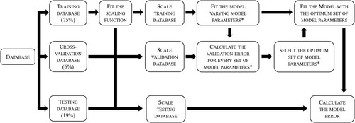
Once the datasets were divided, they were subjected to data scaling. It has been proven that data scaling can improve an ML model performance, reduce the computational time and avoid the possibilities of getting stuck in local minima [50]. A standard scaling function, that standardised the features by removing the mean and scaling to the unit variance, was used. This scaling function was trained by using the training dataset and later applied to the validation and the testing.

After scaling the datasets, the parameters of each of the mentioned models (except the LR model) were tuned. The corresponding hyper-parameters (number of layers and number of nodes per layer for the ANN algorithm, number of decision trees for the RF algorithm and number of trees, decision tree maximum depth and learning rate for the AdaBoost algorithm) were varied over a wide range. For each set of hyper-parameters, the corresponding model was fitted by using the training dataset. After that, the validation error (mean absolute error, MAE) corresponding to that set of hyper-parameters was computed by using the validation database. The optimum set of parameters was selected as the one which would lead to the lowest validation MAE. Once the optimum set of model hyper-parameters was known, the model could be finally fitted with the training dataset and the model MAE could be evaluated by using the testing dataset. The computational time taken for the model hyper-parameters to be optimised and for the final model to be trained were recorded.

Comparing the developed models to previous literature models

Finally, the previously trained models were compared to the empirical models proposed by Steven and Haynes (Equation (1)) [9], Payson and Savage (Equation (2)) [2], Andrews (Equations (3) and (4)) [1], Kung and Rayment (Equations (5) and (6)) [15], van Bohemen (Equation (7)) [6] and Barbier (Equation (8)) [7]. Note that Andrews proposed two different equations, which were named as linear and product models [1]. Also, Kung and Rayment proposed two different models: model 1 and model 2 [15]. (1) $\begin{array}{rl}\text{Ms}& =561.1-473.9w_C-16.7(w_{\text{Cr}}+w_{\text{Ni}})\\ & -21.1w_{\text{Mo}}-33w_{\text{Mn}}\end{array}$(1) (2) $\begin{array}{rl}\text{Ms}& =498.9-316.7w_C-33.3w_{\text{Mn}}-27.8w_{\text{Cr}}\\ & -16.7\ast w_{\text{Ni}}-11.1(w_{\text{Si}}+w_{\text{Mo}}+w_W)\end{array}$(2) (3) $\begin{array}{rl}\text{Ms}& =539-423w_C-30.4w_{\text{Mn}}-17.7w_{\text{Ni}}\\ & -12.1w_{\text{Cr}}-7.5w_{\text{Mo}}\end{array}$(3) (4) $\begin{array}{rl}\text{Ms}& =512-453w_C-16.9w_{\text{Ni}}+15w_{\text{Cr}}-9.5w_{\text{Mo}}\\ & +217w_C^2-71.5w_C\cdot w_{\text{Mn}}-67.6w_C\cdot w_{\text{Cr}}\end{array}$(4) (5) $\begin{array}{rl}\text{Ms}& =539-423w_C-30.4w_{\text{Mn}}-12.1w_{\text{Cr}}\\ & -17.7w_{\text{Ni}}-7.5w_{\text{Mo}}+10w_{\text{Co}}-7.5w_{\text{Si}}\end{array}$(5) (6) $\begin{array}{rl}\text{Ms }& =561-476w_C-33w_{\text{Mn}}-17w_{\text{Cr}}\\ & -17w_{\text{Ni}}-21w_{\text{Mo}}+10w_{\text{Co}}-7.5w_{\text{Si}}\end{array}$(6) (7) $\begin{array}{rl}\text{Ms}& =565-600\ast (1-e^{-0.96w_C})-31w_{\text{Mn}}\\ & -13w_{\text{Si}}-10w_{\text{Cr}}-8w_{\text{Ni}}-12w_{\text{Mo}}\end{array}$(7) (8) $\begin{array}{rl}\text{Ms}& =545-601.2(1-e^{-0.868w_C})-34.4w_{\text{Mn}}\\ & -13.7w_{\text{Si}}-9.2w_{\text{Cr}}-17.3w_{\text{Ni}}-15.4w_{\text{Mo}}\\ & +10.8w_V+4.7w_{\text{Co}}-1.4w_{\text{Al}}-16.3w_{\text{Cu}}\\ & -361w_{\text{Nb}}-2.44w_{\text{Ti}}-3448w_B\end{array}$(8)

These models were built by using very different databases, where their compositional ranges are included in Table 1. As can be observed, most of these models reported in the literature are not valid for many micro-alloying elements, as opposite to the ML models fitted in this work, except the model by Barbier [7]. Because it would not be fair to apply those models to the whole database, for each model, the database (before removing the chemical compositions including Ti, Nb and B) was filtered according to the corresponding literature model compositional range. In that way, for example, alloys including V would not be used to test the accuracy of the Steven and Haynes’ model. Subsequently, the ML models’ MAE and the corresponding literature model’s MAE were evaluated for the filtered database.

Results

Model training and testing

The mentioned ML models were fitted as previously described. The ANN model’s number of hidden layers was selected as 3, where the hidden layers had 5,5 and 3 nodes, respectively. The number of decision trees for the RF model was chosen to be 50. Finally, the AdaBoost model number of decision trees, learning rate and decision tree maximum depth were set as 500, 0.6 and 9, respectively. Table 2 includes the time that was needed to optimise those parameters, considered as the time needed for the calculation of the MAE values given by the different sets of model parameters. As can be seen, the optimisation of the ANN hyper-parameters is more time consuming than the one of the AdaBoost and the RF hyper-parameters, in decreasing order, as it is necessary to optimise more parameters. The LR model does not require of an optimisation.

Table 2. Computational times necessary to optimise the model parameters and to train the ML models used in this work.

	Computational time for
Condition	Model parameters optimisation (s)	Model training (s)
LR	0	0.01
ANN	946.78	9.90
RF	139.50	1.66
AdaBoost	787.32	1.61

Subsequently, models were trained and tested. The trained LR model can be found in Equation (9). The remaining trained models cannot be expressed by equations, as their architecture is more complex. 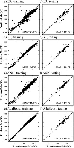(9) $\begin{array}{rl}\text{Ms}& =512-331.3w_C-211.5w_N-31.7w_{\text{Mn}}\\ & -18.1w_{\text{Si}}-8.8w_{\text{Cr}}-16.6w_{\text{Ni}}\\ & -6.8w_{\text{Mo}}+5.5w_V+3.2w_{\text{Co}}-13.3w_{\text{Al}}\\ & -3.0w_W-9.2w_{\text{Cu}}\end{array}$(9) Table 2 includes the time that was needed to train the models, where it can be observed that all of them are very low. Figure 2 includes the predicted vs. experimental Ms plots for all three model, corresponding to the training and to the testing databases. As can be seen, all models fit well the training data, since they all present low training MAE values, always lower than 28°C. The MAE values given when using the testing database are slightly higher, although always similar to the training MAE values, which proves that the models were not over-fitted.

Figure 2. Predicted vs. experimental Ms according to the LR (a, b) ANN (c, d), the RF (e, f) and the AdaBoost (g, h) models. Plots correspond to the training (a, c, e, g) and the testing (b, d, f, h) databases. The dashed lines represent the perfect fit.

Comparison to literature models

Finally, the developed models were compared to previous models in the literature, as previously detailed.

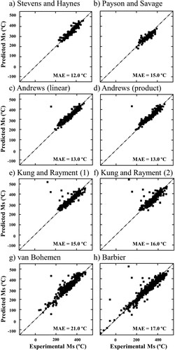
Figure 3 shows a comparison of the MAE values given by the mentioned literature models, always considering the compositional range to which they were built. As can be observed, all MAE values are of the same order of magnitude, regardless of the used model.

Figure 3. MAE values obtained for some literature models, where calculations are made by using a different filtered database for each literature model: (a) Steven and Haynes (213 data-points), (b) Payson and Savage (203 data-points), (c) Andrews (linear model, 307 data-points), (d) Andrews (product model, 307 data-points), (e) Kung and Rayment (model 1, 431 data-points), (f) Kung and Rayment (model 2, 431 data-points), (g) van Bohemen (500 data-points), (h) Barbier (772 data-points). The dashed lines represent the perfect fit.

Discussion

In the last section, three ML models were developed, showing rather low MAE values, of the same order of magnitude than the MAE values obtained by Rahaman et al. [28] when building ML models for the Ms temperature prediction. Although one cannot say what maximum MAE value is acceptable, as it depends on the purpose of the prediction, if one considers any MAE value below 30°C as an indicator of accurate predictions, it can be seen that all the obtained MAE values for the fitted ML models lie in this range. Moreover, the MAE values were always of the same order of magnitude than the LR model. In addition, the results given by the ML models were also very similar to the results given by LR models included in the literature.

With respect to the computational times, it can be noted that the time taken to train the models in this work was negligible, whereas the times taken to optimise the model hyper-parameters was higher, although still not very significant (always lower than 16 min). However, they can be useful as a comparison among the different models, as larger databases can lead to much higher computational times. It is clear that the development of complex ML models requires higher computational times than an LR model.

In addition, the knowledge required to fit an LR model is not as advanced as the knowledge that must be acquired for ML modelling. While both types of models require to know about mathematics and require to understand the relationship among the variables of study, the level of mathematics and coding that is required for ML models is more advanced. Moreover, basic LR models require neither the separation of the database into several datasets nor the optimisation of hyper-parameters. Further understanding on the data can also be done based on ML techniques, which may enable, for instance, to obtain the uncertainty of modelling [51].

The current work has proved that, if the compositional ranges of the database used to build a model are considered, using ML methods does not increase the accuracy of the predictions significantly. Therefore, even though many authors claimed in the past that the performance of models for the prediction of critical temperatures, such as the Ms temperature, can be significantly improved by these recent techniques, it was made clear that these methods are not always necessary. We do not aim to claim that ML modelling is not useful, we think that its capabilities are very wide and this type of models enables to analyse data that could not be analysed before. They can be useful for image recognition and object detection, for identification or use microstructural data or for connecting these microstructural data to processing conditions and property outcomes. However, we think that these models should not be directly considered to be the most accurate ones for problems that can be solved by easier methodologies, such as to prove a relationship between variables or to make inferences from data.

Conclusions

Although it is not denied that ML can be useful for complex problems in materials science, such as image recognition, identification of microstructural data or connection of microstructural data to processing conditions and property outcomes, this work has proved that using ML methods for simple problems, such as the prediction of the Ms temperature, is not necessary. ML methods were proved to require longer computational times, require wider knowledge and lead to similar results, in terms of MAE values. Therefore, we recommend that ML methods are not always considered as the first option when trying to solve easy problems that can be modelled by LR techniques.

Acknowledgements

The authors gratefully acknowledge the support for this work by the European Research Fund for Coal and Steel under the Contract RFCS-2019-899251.

Disclosure statement

No potential conflict of interest was reported by the author(s).

Additional information

Funding

This work was supported by Ministerio de Ciencia e Innovación (MCIN/ AEI /10.13039/501100011033): [Grant Number PID2019-109334RB-C31]; Ministerio de Economía y Competitividad: [Grant Number BES-2017-080945]; Research Fund for Coal and Steel: [Grant Number RFCS-2019-899251]; Research Fund for Coal and Steel: [Grant Number RFCS-2019- 899268].

References

- Andrews KW. Empirical formulae for the calculation of some transformation temperatures. J Iron Steel Inst. 1965;203:721–727.
- Payson P, Savage H. Martensite reactions in alloy steels. Trans Am Soc Met. 1944;33:261–280.
- Peet M. 2007. Materials algorithms project program library. http://www.phase-trans.msm.cam.ac.uk/map/steel/programs/ms-empirical2014.html
- Peet M. Prediction of martensite start temperature. Mater Sci Technol (United Kingdom). 2015;31:1370–1375.
- Sverdlin A V, Ness AR. The effects of alloying elements on the heat treatment of steel. Steel Heat Treat Handb. 1997: 45–91.
- Van Bohemen SMC. Bainite and martensite start temperature calculated with exponential carbon dependence. Mater Sci Technol. 2012;28:487–495.
- Barbier D. Extension of the martensite transformation temperature relation to larger alloying elements and contents. Adv Eng Mater. 2014;16:122–127.
- Wang J, van der Wolk PJ, van der Zwaag S. Determination of martensite start temperature in engineering steels part I. empirical relations describing the effect of steel chemistry. Mater Trans JIM. 2000;41:761–768.
- Steven W, Haynes AGG. The temperature of formation of martensite and bainite in low-alloy steels. J Iron Steel Inst. 1956;183:349–359.
- Carapella LA. Computing A” or ms (transformation temperature on quenching) from analysis. Met Prog. 1944;46(108.
- Grange RA, Stewart HM. The temperature range of martensite formation. Trans ASM AIME. 1946;167:467–501.
- Nehrenberg AE. The temperature range of martensite formation. Trans AIME. 1946;167:494–498.
- Rowland SRL ES. The application of the Ms points to case depth measurements. Trans Of the ASM. 1945;37:27–46.
- Eldis GT, Hagel WC. Effects of microalloying on the hardenability of steel. In: Doane D V, Kirkaldy JS, editor.. hardenability concepts with appl to steel. Chicago, IL: Metallurgical Society of AIME; 1977. p. 397.
- Kung CY, Rayment JJ. An examination of the validity of existing empirical formulae for the calculation of Ms temperature. Met Trans. A. 1982;13.
- Kunitake T. Prediction of Ac1, Ac3 and Ms temperature of steels by empirical formulas. J Japan Soc Heat Treat. 2001;41:164–169.
- Kunitake T, Ohtani H. Calculating the continuous cooling transformation characteristics of steel from its chemical composition. SUMITOMO SEARCH. 1969;2:18–21.
- DeCost BL, Francis T, Holm EA. Exploring the microstructure manifold: image texture representations applied to ultrahigh carbon steel microstructures. Acta Mater. 2017;133:30–40.
- Kusche C, Reclik T, Freund M, et al. Large-area, high-resolution characterisation and classification of damage mechanisms in dual-phase steel using deep learning. PLoS One. 2019;14:e0216493.
- Mulewicz B, Korpala G, Kusiak J, et al. Autonomous interpretation of the microstructure of steels and special alloys. Mater Sci Forum. Trans Tech Publ. 2019;949: 24–31.
- Naik DL, Sajid HU, Kiran R. Texture-based metallurgical phase identification in structural steels: a supervised machine learning approach. Metals (Basel). 2019;9:546.
- Bulgarevich DS, Tsukamoto S, Kasuya T, et al. Automatic steel labeling on certain microstructural constituents with image processing and machine learning tools. Sci Technol Adv Mater. 2019;20:532–542.
- Bulgarevich DS, Tsukamoto S, Kasuya T, et al. Pattern recognition with machine learning on optical microscopy images of typical metallurgical microstructures. Sci Rep. 2018;8:1–8.
- Azimi SM, Britz D, Engstler M, et al. Advanced steel microstructural classification by deep learning methods. Sci Rep. 2018;8:1–14.
- Wang Z, Ogawa T, Adachi Y. Property predictions for dual-phase steels using persistent homology and machine learning. Adv Theory Simulations. 2020;3:1900227.
- Wang Z-L, Ogawa T, Adachi Y. Properties-to-microstructure-to-processing inverse analysis for steels via machine learning. ISIJ Int. 2019.
- Wang Z-L, Adachi Y. Property prediction and properties-to-microstructure inverse analysis of steels by a machine-learning approach. Mater Sci Eng A. 2019;744:661–670.
- Rahaman M, Mu W, Odqvist J, et al. Machine learning to predict the martensite start temperature in steels. Metall Mater Trans A. 2019;50:2081–2091.
- Garcia-Mateo C, Capdevila C, Garcia Caballero F, et al. Artificial neural network modeling for the prediction of critical transformation temperatures in steels. J Mater Sci. 2007;42:5391–5397.
- Capdevila C, Caballero FG, De Andrés CG, et al. Determination of Ms temperature in steels: A Bayesian neural network model. ISIJ Int [Internet. 2002;42:894–902. Available from: http://www.scopus.com/inward/record.url?eid=2-s2.0-0036392448&partnerID=40&md5=6fa2e1747e827795cc91d6634580286a.
- Capdevila C, Caballero FG, de Andrés CG. Analysis of effect of alloying elements on martensite start temperature of steels. Mater Sci Technol. 2003;19:581–586.
- Sourmail T, Garcia-Mateo C. A model for predicting the Ms temperatures of steels. Comput Mater Sci. 2005;34:213–218.
- Sourmail T, Garcia-Mateo C. Critical assessment of models for predicting the Ms temperature of steels. Comput Mater Sci. 2005;34:323–334.
- Vermeulen WG, Morris PF, Weijer Ad, et al. Prediction of the martensite start temperature using artificial neural networks. Ironmak Steelmak. 1996;23:433.
- Ghosh G, Olson GB. Kinetics of FCC→ BCC heterogeneous martensitic nucleation—I. The critical driving force for athermal nucleation. Acta Metall Mater. 1994;42:3361–3370.
- Ghosh G, Olson GB. Kinetics of FCC→ BCC heterogeneous martensitic nucleation—II. thermal activation. Acta Metall Mater. 1994;42:3371–3379.
- Stormvinter A, Borgenstam A, Ågren J. Thermodynamically based prediction of the martensite start temperature for commercial steels. Metall Mater Trans A. 2012;43:3870–3879.
- Pedregosa F, Varoquaux G, Gramfort A, et al. Scikit-learn: machine learning in python. J Mach Learn Res. 2011;12:2825–2830.
- Buitinck L, Louppe G, Blondel M, et al. API design for machine learning software: experiences from the scikit-learn project. arXiv Prepr arXiv13090238. 2013.
- Sourmail T, Garcia-Mateo C. MAP_DATA_STEEL_MS_ (2004). [Internet]. Mater. Algorithms Proj. 2004 [cited 2021 Mar 1]. Available from: https://www.phase-trans.msm.cam.ac.uk/map/data/materials/Ms_data_2004.html.
- Laboratory NPL. MTDATA. Teddington, Middlesex, UK, TW11 0LW; 2003.
- Rumelhart DE, Hinton GE, Williams RJ. Learning representations by back-propagating errors. Nature. 1986;323:533–536.
- LeCun YA, Bottou L, Orr GB, et al. Efficient backprop. neural networks: tricks of the trade. Springer. 2012: 9–48.
- Breiman L. Random forests. Mach Learn. 2001;45:5–32.
- Rokach L, Maimon OZ. Data mining with decision trees: theory and applications. Singapore: World scientific; 2014.
- Breiman L, Friedman J, Stone CJ, et al. Classification and regression trees. London: CRC press; 1984.
- Freund Y, Schapire RE. A decision-theoretic generalization of on-line learning and an application to boosting. J Comput Syst Sci. 1997;55:119–139.
- Drucker H. Improving regressors using boosting techniques. ICML. Citeseer. 1997: 107–115.
- Ripley BD. Pattern recognition and neural networks. Cambridge: Cambridge University Press; 2007.
- Bishop CM. Neural networks for pattern recognition. Oxford: Oxford University Press; 1995.
- Bhadeshia H. Neural networks and information in materials science. Stat Anal Data Min ASA Data Sci J. 2009;1:296–305.