From molecular to continuum modelling of bistable liquid crystal devices

ABSTRACT

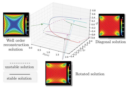
We study nematic equilibria on a square with tangent Dirichlet conditions on the edges, in three different modelling frameworks: (i) the off-lattice Hard Gaussian Overlap and Gay–Berne models; (ii) the lattice-based Lebwohl–Lasher model; and the (iii) two-dimensional Landau-de Gennes model. We compare the modelling predictions, identify regimes of agreement and in the Landau-de Gennes case, find up to 21 different equilibria. Of these, two are physically stable.

GRAPHICAL ABSTRACT

KEYWORDS:

• Bistable liquid crystals
• bifurcation
• Hard Gaussian Overlap (HGO)
• Gay–Berne
• Lebwohl–Lasher
• Landau-de Gennes

1. Introduction

Nematic liquid crystals (LCs) are complex anisotropic liquids that combine the fluidity of liquids with a degree of long-range orientational order characteristic of solids, that is, the constituent nematic molecules typically align along some preferred directions, referred to as directors in the literature [1,2]. Nematics, like most complex materials, can be modelled using both microscopic molecular-level models and continuum phenomenological models. Continuum theories, such as the Oseen–Frank theory or the Landau-de Gennes (LdG) theory, have been hugely successful for nematic LCs, especially in the context of spatially inhomogeneous confined systems. Molecular-level theories that incorporate details about the molecular shape and molecular interactions have also been used to simulate spatially homogeneous systems to estimate bulk properties or transition temperatures [3,4]. As experimentalists are able to design severely confined systems, it is desirable to simulate spatially inhomogeneous systems with more detailed molecular-level models which are computationally intensive, since the validity of continuum descriptions is not clear for small systems. We model a toy confined nematic system with boundaries using three different approaches – two off-lattice molecular-level models, one lattice-based mesoscopic-level model and the continuum (macroscopic) LdG model, ordered in terms of decreasing detail. The purpose is to firstly simulate an inhomogeneous system with molecular-level models on a regular desktop computer and ascertain the limits of what can be achieved and then compare it to less detailed computational approaches. Secondly, we want to identify regimes of correspondence between the three different modelling regimes, that is, where do the model predictions match, where do they differ, and how do we interpret the differences. Such exercises may allow us to precisely define limits of applicability for coarse-grained theories and design new multiscale methods that can effectively couple molecular, lattice-based and continuum approaches [5,6].

We re-visit the square wells filled with nematic LCs, reported by Tsakonas et al. [7], where the authors design a prototype LC system comprising a periodic array of three-dimensional (3D) shallow wells filled with nematic LCs. The experimental work is accompanied by two-dimensional (2D) LdG modelling in [7] and the authors numerically reproduce the diagonal and rotated solutions. These wells have a square cross section and are typically shallow with the vertical dimension being smaller than the cross-section dimension. Typical well dimensions are or μm. The well surfaces are treated so as to induce planar degenerate conditions on the well surfaces i.e. the nematic molecules on the surfaces prefer to be in the plane of the surfaces. Therefore, the molecules are preferentially tangent to the edges where two well surfaces meet i.e. if we orient a square well along a standard Cartesian frame of reference centred at the bottom left well vertex, then the molecules prefer to align in the x-direction on the edges common to the faces in the xy and xz-planes. This induces a natural mismatch in the molecular orientations at the well vertices where three edges intersect.

Tsakonas et al. [7] experimentally observe at least two nematic equilibria, both of which have long-term stability without an external field. They observe that the experimentally observed profiles are invariant across the height of the well, for shallow square wells and it suffices to examine the profile on the bottom square cross section. They observe a diagonal solution where the molecules, on average, align along a diagonal on the square cross section and a rotated solution for which the molecules, on average, rotate by radians between a pair of opposite square edges. There are two diagonal solutions and four rotated solutions, so the wells are truly multistable. The experimental work in Tsakonas et al. [7] is accompanied by two-dimensional (2D) LdG modelling and the authors numerically reproduce the diagonal and rotated solutions.

The work in Tsakonas et al. [7] has been vigorously followed up in the continuum framework. The continuum theories generally have an associated energy functional and the experimentally observed equilibria are modelled by energy minimisers although there may be multiple unstable equilibria that correspond to non-energy minimising critical points of the continuum energy. Lewis et al. [8] report similar experimental observations for viruses confined to rectangular chambers and the authors compute semi-analytic expressions for the diagonal and rotated solutions in the simpler continuum Oseen–Frank framework. Luo et al. [9] study the diagonal and rotated solutions as a function of the anchoring strength in a 2D LdG framework, which is a measure of how strongly the tangent conditions are enforced on the well surfaces. They compute a bifurcation diagram which suggests that the rotated solutions can only be observed if the anchoring is greater than a material-dependent and temperature-dependent critical threshold and hence, rotated solutions are not as ubiquitous as the diagonal solutions. Kusumaatmaja and Majumdar [10] study the solution landscape in the 2D LdG framework and compute the transient states or unstable critical points of the LdG energy that connect the stable diagonal and rotated solutions in the LdG framework. Kralj and Majumdar [11] adopt a 3D LdG model and find a novel well-order reconstruction solution (WORS), in addition to the conventional diagonal and rotated solutions, when the well cross section is comparable to a material-dependent and temperature-dependent characteristic length scale, referred to as the biaxial correlation length , that is, when the well cross section, D, is and the critical depends on both the material and the temperature. In some cases, could be 7 and in other cases, could be as large as 20. The work in Tsakonas et al. [7] has motivated authors to consider more complex geometries and the effects of nematic confinement therein [12] and to study patterned geometries with mixed boundary conditions such as a combination of tangent and normal boundary conditions [13]. Davidson and Mottram [14] use a Schwarz–Christoffel conformal mapping technique to show that these methods can be used to simulate switching behaviour of a nematic confined in a 2D square well. Gârlea and Mulder [15] simulate long rod-like lyotropic molecules in a quasi-2D square geometry, using a Metropolis Monte Carlo method and hard rods with length times the size of the domain. They found a single fixed lens-shaped pattern similar to the diagonal solution in [7]. Slavinec et al. [16] use a 3D molecular-level Lebwohl–Lasher (LL) model in a confined square well to show that the nematic structure is effectively two-dimensional. Most of the modelling to date has been done in the continuum framework and the continuum modelling reveals the rich solution landscape and how the landscape can be manipulated by geometry, temperature, material properties, boundary effects and external fields.

This paper compares both molecular-level and continuum LdG models of these nematic-filled wells, using off-lattice molecular-level Hard Gaussian Overlap (HGO) and Gay–Berne (GB) models, a lattice-based LL model and a continuum LdG model. These models are ordered in terms of decreasing detail and decreasing computational complexity. The molecular-level models contain information about the molecular shape and nature of molecular interactions and are therefore well-suited to describe the effect of microscopic interactions on averaged quantities of interest. The LdG model parameters are largely phenomenological and we have not been able to trace clear empirical relations between the LdG model parameters and the parameters in the molecular-level models. These models are described in detail in the next sections. We take our computational domain to be a square in all cases and compute averaged quantities of interest in the molecular framework and the macroscopic order parameter fields in the LdG framework. We do not recover the rotated solution with the off-lattice models but only observe the diagonal and 2D variants of the WORS in the off-lattice case. This is consistent with continuum results which show that rotated solutions have higher energies than diagonal solutions and are unstable at small well sizes. We perform a temperature sweep of the LL model and study the emergence of diagonal and rotated solutions from disordered solutions as the temperature decreases. In the 2D LdG framework, we compute a detailed bifurcation diagram of the LdG solutions as a function of the well size. We numerically demonstrate the existence of hitherto unreported LdG equilibria, which have multiple interior defects and though unstable, can be of importance in transient dynamics. In a particular case, we find 81 LdG equilibria on a square with tangent boundary conditions, of which only the conventional diagonal and rotated solutions are stable. Whilst performing three parallel numerical studies, we identify regimes of qualitative agreement between the molecular-level, mesoscopic and continuum models and we hope that the presented results will constitute the foundation for more detailed model comparisons in the future.

2. Microscopic and mesoscopic molecular-level models

In this section, we review two off-lattice molecular-level models: the HGO [17] and GB models [18], respectively, and one lattice-based mesoscopic model, the LL model [19] for nematic LCs. In the off-lattice and lattice-based simulations, we measure length in units of , where nm is the assumed width of the nematic molecules. The computational domain is a square box with side length, for the off-lattice simulations and for the lattice-based simulation, and the number of molecules, N, is calculated in terms of average density to be . We impose a molecular version of planar Dirichlet boundary conditions along the square edges, that is, we place a line of molecules along each edge whose orientations are tangent to the edge in question and the position and orientation of these boundary molecules are fixed in time. For both classes of models, we compute nematic equilibria on squares, with the fixed planar boundary conditions on the edges using Markov chain Monte Carlo (MCMC) methods that are described in detail in Section 3. We only find the diagonal solution or some variant of the diagonal solution with the off-lattice simulations and do not recover the rotated solution. A further interesting feature of the off-lattice simulations is the asymmetric nature of the corner defects i.e. the off-lattice simulations show that some corner defects are more pronounced than others in the sense that the associated regions of reduced nematic order are larger for some corners than for others and this has not been previously captured by continuum simulations. Continuum simulations show that all four vertices are equivalent. The lattice-based simulations are less computationally demanding and we perform a more systematic parameter sweep with the LL model, capturing the emergence of both the diagonal and rotated solution branches as we vary model parameters.

2.1 HGO and GB models

The off-lattice models describe the nematic state by the molecular positions and orientations, , where is the location of the ith molecule and the unit vector, , is the orientation of the ith molecule, N, see Figure 1(a).

Figure 1. (a) A schematic of off-lattice HGO and GB models. The potential between two particles is described using their orientations ( and ) and relative position . The width of each particle is set to . (b) A schematic of lattice-based LL model. The orientation of particle i is given by and the lattice spacing is set to .

The HGO model is a hard particle model based on purely repulsive forces and excluded-volume effects between the interacting LC molecules; see [4] for applications of the HGO model in the context of LCs. The HGO model prescribes an intermolecular potential which is infinite for overlapping molecules and is zero for non-overlapping molecules. In Section 3, we apply MCMC simulations to estimate the equilibrium properties of the HGO model. If we considered time-dependent simulations, the HGO intermolecular potential would translate into a free movement of a molecule until it collides with another molecule [20]. By only considering equilibrium properties, the molecular-level model requires less parameters, but it cannot provide dynamic information. The same is also true for continuum models. For example, Luo et al. [9] propose a dynamic model for the switching mechanisms between rotated and diagonal states in the LdG framework by introducing an additional parameter, effectively controlling the characteristic timescale.

LC molecules are labelled as being overlapping when the distance between their centres of masses is less than an explicitly prescribed shape parameter, . We take the shape parameter, , of the HGO model to be identical to the GB shape parameter and hence, one can compare the HGO and GB models. The HGO potential, , between a pair of molecules, i and j, is a function of the molecular orientations , and , where and are positions of molecules and , and is given by

where and . The shape parameter , also referred to as the range parameter, is the interaction distance between two ellipsoids taken from the Gaussian overlap model of Berne [21]:

(1)

The parameter is a molecular property, related to the shape anisotropy by

where is a measure of the molecular aspect ratio and , are proportional to the length and width of the molecules, respectively. More precisely, and are the distances at which the GB potential (see Equation (2)) is zero when the two interacting molecules are in the end-to-end or the side-by-side configurations, respectively.

The GB model is one of the most successful off-lattice models for nematic LCs. It has (at least) four tuning parameters and has thus the potential of simulating a wide range of liquid crystalline materials, perhaps more so than the HGO model which has fewer tunable parameters. The GB intermolecular potential, , is a soft-core Lennard–Jones type potential, with both attractive and repulsive components, given in [18] by

(2)

The first term is an energetic term and the second term is a Lennard–Jones type contribution with both attractive and repulsive contributions. Here

where the range parameter is identical to Equation (1) in the HGO model. The energy term in Equation (2) is written as

where

and

where is the well-depth ratio for the end-to-end and side-by-side configurations, and well-depth refers to the depth of the Lennard–Jones potential well.

The four tuning parameters of the GB model are , and we work with the commonly used set of values [4]. These values have been successfully used to reproduce the nematic-isotropic phase transition in homogeneous samples [22], and it is reasonable to use them to simulate inhomogeneous samples too. We note that the GB model has more parameters and a complex energetic structure compared to the HGO model, and although we use the same algorithm to simulate both models, we cannot expect the same results. In fact, the differences between the two sets of results may be useful for understanding the relative importance of the tunable parameters in the GB model.

2.2 LL lattice-based model

The LL model is a lattice-based model for nematic LCs, based on the principle that clusters of molecules are pinned at the sites of a regularly spaced lattice and interact with their nearest neighbours [19]. Such models suppress the translational freedom of molecules and inevitably contain less physics than the off-lattice models, but are relatively computationally tractable, making them a good compromise or even a (mesoscopic) bridge between molecular (microscopic) and continuum (macroscopic) theories. In Figure 1(b), we impose a 2D square lattice of spacing (in units of ) on the computational domain and the LL potential is then given by

where L is a measure of the strength of intermolecular interactions (we take ), i, j are indices for neighbouring lattice sites, and are the respective cluster orientations and the sum is taken over all pairs of connected lattice sites. The potential, , is minimised when for all i and j, that is, in the case of perfect alignment.

The LL model is one the simplest lattice models in the literature and there are several variants and generalisations which include more complex interactions [23,24]. However, the presented LL model is a good benchmark for lattice-based approaches (i.e. how do they compare to other approaches) and suffices for the purposes of this paper.

3. Numerical methods: Monte Carlo simulations

We use a MCMC method to find minimisers of the HGO, GB and LL potentials, using the Metropolis–Hastings algorithm [25]. This algorithm takes individual samples from a high-dimensional probability distribution representing the likelihood of different particle configurations. Each sample is close (in configuration space) to the previous sample in the chain, but the particular chain of samples does not represent physical time. Nevertheless, the analogy comparing the chain of samples to time is a useful one, and we will make use of this for the remainder of the paper. For example, ‘transient behaviour’ refers to changes in particle configuration along the chain of samples, and ‘temporal averaging’ refers to averaging over a section of this chain.

For the off-lattice models (HGO and GB), at each step of the algorithm, we randomly choose a molecule i and alter its position and orientation using random variables uniformly distributed between and , respectively. The lattice case operates similarly but without altering the position. We define the corresponding perturbations by and , respectively, and the updated positions and orientations are given by

The change in potential energy, , is given by

where and . The proposed move is accepted with probability (for ), where T is a dimensionless re-scaled temperature [26] and rejected otherwise (for ). For the off-lattice simulations, we use in our acceptance criterion, following the values used in [26]; we do not relate this temperature to physical temperature or the temperature variables used in continuum models. If the move is accepted, then we continue the algorithm with the updated positions and orientations, and if not, the previous values of are retained.

We perform passes of the MCMC algorithm and each pass comprises N random moves, where N is the number of nematic molecules. We perform spatial averaging over the molecular orientations to obtain a Q-tensor (see next paragraph) after every 10 passes. At the end of the algorithm, we take the arithmetic average of the Q-tensor fields to yield a temporally averaged configuration. We expect the temporally averaged configuration, computed at the end of passes, to approximate the stationary solutions for sufficiently large . Our simulations suggest that we typically need to compute stationary solutions or solutions which seem to be in equilibrium for off-lattice models.

We compute the spatially averaged two-dimensional Q-tensor over an artificial lattice with spacing , and calculate a spatial average within a circle of fixed diameter around each lattice site, to obtain the Q-tensor, where m is the particle orientation and is the Kronecker delta symbol. By means of comparison with the continuum LdG theory, the Q-tensor can be rewritten in terms of the scalar order parameter s, a measure of the degree of orientational order, and the director n, or the locally preferred average orientation i.e. where n is the principal eigenvector with the positive eigenvalue, s. The averaging procedure yields Q, with two independent components, and . We extract s and n from the numerical data by using the relations

If , then we simply set . From the averaged definition of Q above, and describes isotropic or disordered regions that are typically associated with defects. We present some prototypical simulation results for the off-lattice models in Section 4.

In the case of the lattice-based LL model, we use the same MCMC algorithm as for the off-lattice models. The temperature in the acceptance criterion of the LL model cannot be related to the acceptance criterion in the GB model, since the LL temperature is weighted by the interaction parameter L and we cannot precisely relate L to the GB parameters. As in the off-lattice case, we perform spatial and temporal averaging to obtain the director, n, and order parameter, s, as outlined above. Here, the spatial averaging is done over neighbouring lattice sites (as opposed to a disc in the off-lattice case) and the temporal averaging is done after passes of the MCMC algorithm.

4. Results of MCMC simulations

The off-lattice simulations are computationally expensive and the runs can take up to a week on a regular desktop computer. We typically need passes to attain a quasi-stationary configuration and there is no perceptible change or movement in the temporally averaged Q-tensor after passes. We terminate the algorithm after passes. The number of molecules, and , for this set of parameter values. We have performed some parallel simulations with in the off-lattice framework and the qualitative conclusions remain unchanged (compare Figures 2 and 3).

Figure 2. Typical configuration for HGO off-lattice model. After averaging over passes, the solutions are not stationary and the top and bottom rows show two example configurations. Plots on the left show a single particle configuration, while plots on the right show the spatially and temporally averaged s and director fields over the passes. Parameters are , , and .

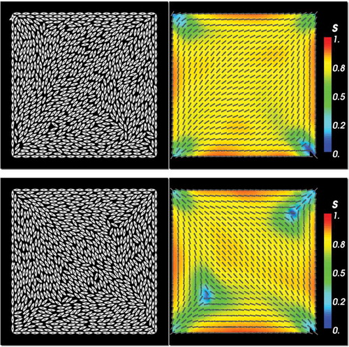
In Figure 2, we plot two different particle configurations for the HGO model in the left column and the spatially and temporally averaged n and s fields after passes in the right column. The solutions are not stationary after 10⁵ passes. The instantaneous molecular configurations do not exhibit a noticeable degree of ordering for the ellipsoidal particles. The averaged configurations exhibit a largely diagonally oriented pattern for n, with away from the four vertices. The order parameter drops drastically near the vertices, with near the corners. Further, the regions of reduced order fluctuate in size, as can be seen by comparing the two snapshots in the right column, and individual defects of reduced order can break away from the corner and move into the centre of the domain. In both cases, the regions of reduced order are asymmetrically distributed between the four vertices and there is a distinct difference between ‘splay’ vertices and ‘bend’ vertices. The splay vertices are associated with a radial or splay director profile (see the bottom right and top left vertex in the bottom right snapshot in Figure 2) and the director field bends around a bend vertex, as in the bottom left and top right vertices of the bottom right panel in Figure 2. The ‘bend’ vertices have a larger neighbourhood of reduced order and these regions can stretch along almost a third of the domain width (e.g. lower right plot in Figure 2), or retreat to become point defects at the corners (e.g. upper right plot in Figure 2). This is in line with the diagonal solutions reported in experimental work and macroscopic LdG models for this problem [9], and we expect to see reduced order near the vertices, originating from the mismatch in molecular alignments at the vertices.

We increase the number of MCMC passes to and find a stationary n field, as shown in Figure 4(a). This shows a clear diagonal ordering pattern with corner defects. In contrast to the numerical results for LdG models in the literature [9], the vertex profiles vary significantly. There are two pairs of vertices as described above. The ‘splay’ vertices are highly localised neighbourhoods of reduced order whereas there are clear defect lines (with ) emanating from the ‘bend’ vertices, and the neighbourhoods of reduced order (i.e. with lower s) are larger than for the ‘splay’ vertices. We have not observed the rotated solution in the HGO simulations.

Figure 3. Typical configuration for HGO off-lattice model for a larger number, , of simulated molecules. The plot on the left shows a single particle configuration, while the plot on the right shows the spatially and temporally averaged s and director fields over the passes. Other parameters are as in Figure 2.

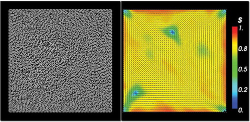
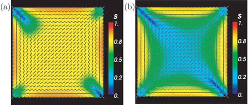
Figure 4. (a) Stationary configuration for HGO off-lattice model. Stationary s and director fields are obtained by averaging over an increased number of passes . Parameters are , , and . (b) Stationary configuration for the GB off-lattice model. Parameters are , , , , , , , and .

We repeat the same simulations (using ) with the GB model. The results are qualitatively similar to the HGO model, in the sense that we obtain a non-stationary diagonal orientation pattern for passes with point defects and defect lines emanating from each vertex, some of which are longer than those observed in the HGO model and traverse almost half the diagonal length, see Figure 5. We obtain a stationary solution for passes, as illustrated in Figure 4(b). There are differences compared to the HGO stationary solution. The diagonal pattern is localised near the centre of the square surrounded by a constant eigenframe pattern where the molecules are effectively oriented tangent to the edges. There is reduced order near the centre of the square, there are defect lines emanating from the ‘bend’ vertices and the asymmetry between the splay and bend vertices is evident. The degree of order is maximal near the edges. We can provide a partial explanation for this stationary pattern based on numerical observations of the MCMC iterations. 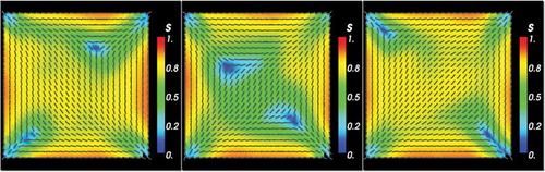The diagonal pattern switches its primary orientation by 90° after approximately passes, halfway through the cycle of 10⁸ passes, as shown in Figure 6. We conjecture that the reduced order near the square centre and the constant eigenframe away from the centre (such that n effectively follows the square edges in this region) could follow from the superposition of the two different diagonal solutions. This could be a microscopic explanation for the WORS reported for the continuum LdG model in [11].

Figure 5. Typical configuration for GB off-lattice model. After averaging over passes, the solutions are not stationary and the top and bottom rows show two example configurations. Plots on the left show a single particle configuration, while plots on the right show the spatially and temporally averaged s and director fields over the passes. Parameters are , , , , , , and .

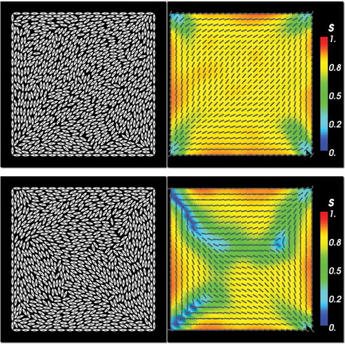
Figure 6. Sequence of averaged configurations showing switching between diagonal solutions in the GB off-lattice model. The plots show a sequence of three different averages, each using passes, over a total of passes of the MCMC algorithm. Parameters are , , , , , , and .

In both cases (HGO and GB models), we fail to recover the rotated solution and both models suggest differences between the defect structures at ‘splay’ and ‘bend’ vertices. The ‘bend’ vertices have a longer persistence length for reduced order. The two off-lattice models yield somewhat different stationary solutions. The HGO model yields the conventional diagonal solution whilst the GB model yields a superposition of two different diagonal solutions, with a reduced square of smaller s near the centre. The GB stationary solution is more reminiscent of the continuum WORS. We conjecture that the HGO and GB models (for the parameter values employed here) correspond to different parameter regimes of the continuum approach and hence, yield different stationary solutions. In the absence of a rigorous off-lattice to continuum derivation, it is difficult to give precise reasons for these differences.

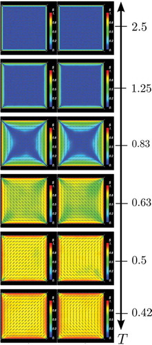
The mesoscopic lattice-based LL model can yield both the diagonal and rotated solutions, see bottom left and right panels in Figure 7, respectively, although diagonal solutions are still more common. For example, we have performed 100 simulations using different random initial conditions for the lattice director in the LL framework, at a fixed temperature . In 88 out of these 100 simulations, we have found a stationary diagonal solution and for the remaining 12, we have found a stationary rotated solution. In Figure 7, we report results of a temperature sweep, where we compute the stationary equilibria of the LL model as the system temperature T is varied between . There is no systematic reason for this choice of temperatures except that the sweep captures the transition from disordered equilibria at high temperatures to the conventional diagonal and rotated solutions at lower temperatures. For each temperature, we run two simulations, with a diagonal and rotated initial condition respectively. These initial conditions are obtained from the continuum LdG model solved in Section 5. For higher temperatures around or higher, the system tends towards a largely disordered steady state with almost everywhere, except near the edges where we have imposed a molecular version of Dirichlet boundary conditions. As the temperature is decreased to , we recover the GB stationary solution in the sense we have a constant eigenframe near the edges and an interior square-like region of low order and largely diagonal director field. There is no visible asymmetry between the four vertices and we cannot make a distinction between ‘splay’ and ‘bend’ vertices. For , the disordered regions with disappear and the order parameter over the whole domain. We solely recover the diagonal solution in this regime, irrespective of the initial condition. As T further decreases, say for , the steady state randomly approaches either a diagonal or a rotated solution. There are no marked differences between the vertex profiles at the ‘splay’ and ‘bend’ vertices. For , we recover the familiar diagonal and rotated solutions as seen in the continuum model and the stationary solution is dictated by the initial condition, that is, if the initial condition is the continuum diagonal solution, the final stationary LL solution is also the diagonal solution and similar remarks apply to the rotated solution.

Figure 7. In each column, temperature parameter sweep for the lattice-based LL model. In each row, the MCMC simulations were run with either a D1-solution (left column) or a R1-solution (right column) of the continuum LdG model used as the initial condition. Each row corresponds with a different value for the (dimensionless and re-scaled) temperature T. Parameters are , and .

5. LdG model

The last part of this paper focuses on the LdG model in two dimensions. As mentioned in Section 1, the LdG theory is one of the most successful continuum theories for nematic LCs and describes the state of a nematic by a macroscopic order parameter, the Q-tensor, which is defined in terms of macroscopic quantities such as the dielectric anisotropy or the magnetic susceptibility [1]. The LdG Q-tensor can be viewed as a macroscopic measure of anisotropy or degree of orientational order. The LdG Q-tensor need not necessarily agree with the mean-field Q-tensor defined in Section 3. In fact, the LdG order parameters can take values greater than unity for low temperatures [27] whereas the mean-field order parameters are less than unity, and the LdG theory is known to fail near critical temperatures, near defects and interfaces. In spite of some limitations, the LdG theory has been used in the literature to study nematic equilibria in square wells [7,9,11,28]. We build on the existing work by conducting a numerical study of solution branches and their stability as a function of domain size and this yields novel insight into the emergence of bistability and multistability in these devices.

We adopt a strictly 2D approach to LdG equilibria on the square domain, that is, we describe the nematic state by a symmetric, traceless 2 × 2 matrix, which can be written as

with two degrees of freedom, . This can be thought of as a modified Ericksen approach for uniaxial nematic phases, that can be fully described by a 2D unit-vector field, n, and a scalar order parameter, s, that accounts for the degree of orientational order about n; similar approaches have been successfully used in [7,9] and [10]. The degrees of freedom vector, , is related to the director, , and the scalar order parameter, s, by and The LdG theory is a variational theory and observable equilibria correspond to minimisers of an appropriately defined LdG energy [2]. We work with a particularly simple form of the LdG energy density, comprising the one-constant elastic energy density and a non-convex bulk potential as shown in the following:

where , is the square edge length in units of micrometres and

L is a material-dependent elastic constant, A is the re-scaled temperature and and are positive material-dependent constants. For such 2 × 2 matrices, and . We work at a fixed temperature below the critical supercooling temperature so that and the bulk potential, , is a minimum for . We non-dimensionalise the LdG energy using the scalings , , and define the following dimensionless LdG energy [9]:

(3)

where is the gradient with respect to the re-scaled coordinates, is the unit square and . In what follows, we fix , L and vary D; this has the same effect as varying the temperature A if D and L were kept fixed. In other words, we can either increase D or increase (move to lower temperatures) and both parameter sweeps are equivalent to decreasing and investigating structural changes in the limit.

On the boundary, we prescribe Dirichlet boundary conditions, consistent with the tangent boundary conditions which require that is an integer multiple of on the horizontal edges and that is an odd integer multiple of on the vertical edges. Following [9], these conditions translate to: for horizontal edges, for vertical edges and for . Local minimisers of Equation (3) are solutions of the corresponding weak formulation [9], given by

(4)

(5)

where and are arbitrary test functions. There are generally six different solutions to Equations (4) and (5), two diagonal, D1–D2, and four rotated, R1–R4, states. Examples of D1 and R1 can be seen in the bottom row of Figure 8, and the remainder (D2, R2–R4) are simply rotated versions of D1 and R1. All six solutions can be generated using a finite element discretisation, with suitable initial conditions [9] by computing solutions of the Laplace equation subject to the boundary conditions shown in Table 1. The initial Q tensor field is then constructed from , where at the interior nodes and at the boundary nodes. As in [9], we define g by a trapezoidal function that smoothly decays to zero at each vertex, to avoid discontinuities at the square vertices:

Table 1. Dirichlet boundary conditions resulting in optimal solutions D1–D2 and R1–R4.

Solution
D1			0	0
D2
R1				0
R2			0
R3
R4

where

Once we define the six distinct initial Q-tensor conditions, we use these initial fields to solve Equations (4) and (5) using the FEniCS package [29,30]. Lagrange elements of order 1 are used for the spatial discritisation, and the resulting non-linear system of equations are solved using a Newton solver (with a linear LU solver for each iteration).

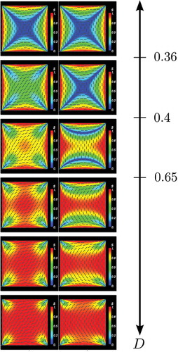
Figure 8. Bifurcation solutions for the LdG model for a D1-solution (left column) and for a R1-solution (right column). The values for D for each column are 0.90, 1.20 μm. The tick marks on the D-axis show the approximate locations of the solution bifurcations, for example, the first bifurcation from the single stable WORS solution to the stable diagonal and unstable WORS solutions occurs at .

We have performed a similar parameter sweep as has been done for the LL model in Figure 7. The results for the LdG model are reported in Figure 8. The LdG model is at a fixed temperature below the nematic–isotropic phase transition and we investigate structural changes by varying the domain size D. We use typical values , Nm and N/m [31] in the definition of above. We perform a continuous parameter sweep in terms of μm, using two different initial conditions – the D1 and R1 initial Q-tensor fields constructed above (refer to Table 1). For μm, we uniquely recover a 2D (2D) version of WORS reported in [11], irrespective of the initial condition. This 2D WORS is characterised by an isotropic cross (with ) connecting the four square vertices along the two square diagonals. The cross partitions the square into four quadrants and n is constant in each quadrant, that is, n is either the unit-vector in the x-direction if the quadrant contains a horizontal edge or n is the unit-vector in the y-direction if the quadrant contains a vertical edge. For μm, we get the diagonal solution with the D1 initial condition and the rotated solution with the R1 initial condition as expected and there are no appreciable structural changes for larger values of D.

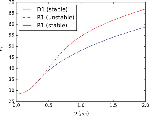
For each value of D, we calculate the stability of the final solution in terms of the smallest real eigenvalue of the Jacobian of the right-hand side (RHS) of Equations (4) and (5). This is comparable to a linear stability analysis and we interpret a zero or positive eigenvalue as a signature of instability and a spectrum of negative eigenvalues as a numerical demonstration of linear stability. A sample of solutions with varying D is shown in Figure 8 for both initial conditions and we compare the respective energies, versus D in Figure 9. It is clear the D1 and R1 solutions branches coincide for small D, separate at some critical value of D and the R1 branch always has higher energy than the D1 branch, consistent with the fact that the D1 solution is more frequently observed in experiments than the R1 solution [8].

Figure 9. (Colour online) Total LdG energy for the R1 and D1 solutions plotted against domain size D. The blue/red lines correspond to the diagonal/rotated solutions presented in Figure 8 (left/right column). Solid lines indicate a stable solution branch, while dashed lines indicate an unstable solution branch.

Next, we discuss the diagonal and rotated solution branches separately. For small D, the D1 initial condition converges to the 2D WORS. This is expected since one can analytically prove that there is a unique equilibrium in the limit. Moreover, Majumdar et al. [32] prove the existence of a 3D WORS on a square with tangent boundary conditions for all values of D. On similar grounds, one would expect that the 2D WORS exists for all values of D and is the unique globally stable equilibrium for small D.

As D increases, the D1 initial condition converges to a more diagonally ordered solution with isotropic lines originating from the four vertices. In contrast to the off-lattice (HGO or GB) simulations, all four vertices have identical order profiles. For example, for μm, the D1 solution has almost everywhere in the square domain except near the vertices. As D further increases, the D1 solutions maintain the diagonal profile but have enhanced interior order and the regions of low order retreat to the vertices. As D further increases, the interior order parameter almost approaches the maximal value 1, the director profile is prominently diagonal and there are localised small regions of reduced order near the vertices. The D1 solutions are always numerically stable and have lower energy than the corresponding R1 solutions (see Figure 8).

We perform a parallel numerical study of LdG equilibria with the R1 initial conditions. The R1 branch converges to the 2D WORS for small D. From Figure 8, we deduce that there exists a bifurcation point at some μm such that the 2D WORS is the unique solution (and hence stable) for , is unstable for (from numerical computations the 2D WORS exists for all ) and the stable D1 solution branch appears for . There are multiple equilibria for and the R1 branch and the D1 branch separate at . The R1 solutions are unstable for intermediate values of D or for D close to ; they separate from the 2D WORS branch and lose the isotropic cross as D increases. As D increases, the isotropic cross deforms to localised transition layers (with ) near a pair of opposite square edges. The transition layers partition the square into three distinct regions and n is approximately constant in each region, determined by whether the region contains horizontal or vertical square edges (see third panel in Figure 8).

For m, the R1 solution converges to the familiar rotated solution. The director has a visibly rotated profile, the order parameter s is approximately unity in the square interior and there are localised regions of reduced order near the vertices, originating from the mismatch in the imposed Dirichlet conditions. Again, there is no perceptible asymmetry in the order profiles for the four vertices. For D close to 1 μm, the R1 solutions are numerically stable (see Figure 9). Hence, our numerical search suggests that the R1 solutions follow the 2D WORS for , follow a different unstable solution branch characterised by localised edge transition layers for and then follow the stable rotated solution branch, which seems to exist only for .

In the continuum simulations, we do not find solutions that demonstrate an interior diagonally ordered profile (with small s) surrounded by a constant eigenframe solution, with n tangent to the square boundary as in the GB simulations or some of the LL simulations at intermediate temperatures. The 2D WORS could be interpreted as the continuum counterpart of these molecular solutions, in the sense that the 2D WORS has an interior region of reduced order (small values of s) around the centre of the square and has a constant eigenframe (i.e. n is constant) almost everywhere inside the square.

We conclude this section by computing a bifurcation diagram of the LdG solution branches as a function of D. We start be defining two new measures and , and then solve the LdG equations using, as initial conditions, each of the six previously identified solutions (i.e. D1–D2 and R1–R4). We then calculate and from the final solution and plot these measures versus D, again using solid/dashed lines for stable/unstable branches. Using the new measures and enables us to visualise each solution branch separately. The detailed bifurcation diagram in Figure 9 illustrates the qualitative features mentioned above: the unique 2D WORS for small D, a bifurcation at some critical ; the 2D WORS exists as an unstable solution branch for and there are two further new stable solution and unstable solutions branches, respectively. The rotated solution branches in Figure 7 follow the unstable solution branches. There is at least another critical value, at which each unstable solution branch bifurcates into two stable solution branches. These stable solution branches are the conventional rotated solutions, yielding a total of four numerically stable rotated solutions for as expected.

The solution landscape and the multiplicity of equilibria near the critical point is not clear from Figure 9. In an attempt to identify the distinct equilibria of the system as D is varied, we apply the deflated continuation algorithm of Farrell et al. [33] to the LdG model. In contrast to the classical bifurcation analysis algorithm of Keller [34], deflated continuation is capable of computing connected and disconnected bifurcation diagrams and does not require the solution of nonscalable subproblems, allowing it to scale to fine discretisations of partial differential equations.

At the heart of the algorithm is a deflation technique for discovering distinct solutions to nonlinear problems [35]. Let be the discretised residual of a nonlinear PDE, and suppose that k distinct solutions are known for this problem, that is, for all . We construct a new nonlinear problem via

This deflated problem has two properties of interest. First, any solution of G not in is also a solution of F. Second, Newton’s method will not converge to the known solutions Q from any initial guess, as long as each known solution satisfies some mild regularity conditions. Thus, if Newton’s method converges from some initial guess, it must have converged to a previously unknown solution; this solution can also be deflated and the process repeated. In this way, deflation allows for the discovery of several solutions from the same initial guess. Deflation and nested iteration were combined in [36] to investigate distinct solutions of an Oseen–Frank LC model.

This is used to compute bifurcation diagrams as follows. Given a set of solutions at parameter value , we wish to compute the set of solutions for . The algorithm proceeds in two phases. In the first phase, each known branch is continued from to : each previous solution is used as initial guess for Newton’s method, yielding . In the second phase, new solutions are sought, such as those arising via a bifurcation on a known branch, or on other disconnected branches that have come into existence between and . All known solutions for are deflated, and each solution at is used again as initial guess for Newton’s method. If Newton’s method succeeds, a new solution has been discovered, and Newton’s method is attempted from that initial guess once more. When Newton’s method has failed from all available initial guesses, the algorithm increments the value of D and repeats the process. For more details, see [33].

For the bifurcation problem of current interest, it is reasonable to start from the single known WORS solution at small D and apply deflated continuation to compute the solutions for larger values of D. Using deflated continuation we find 81 different LdG equilibria at μm, of which only the conventional diagonal and rotated solutions are stable. Once rotational symmetries are discarded, 21 solutions remain, which are shown in Figure 11 ordered by increasingly large values for the largest eigenvalue of the Jacobian of the RHS of Equations (4) and (5) (values of are given in Table 2). We expect that those equilibria with lesser eigenvalues (i.e. ordered soonest) will contribute more to the transient dynamics.

Table 2. The largest eigenvalue of the Jacobian of the RHS of equation Equations (4) and (5) is given here for each panel of Figure 10, where the panel numbers are ordered from left to right and top to bottom.

Panel no.		Panel no.
1	–16.0	12	64.5
2	–15.6	13	65.2
3	10.6	14	66.0
4	11.4	15	92.1
5	11.4	16	115.1
6	15.3	17	120.9
7	15.3	18	121.0
8	22.1	19	121.7
9	22.1	20	121.7
10	30.9	21	225.6
11	60.0

Figure 10. (Colour online) Bifurcation diagram for the LdG model, plotting averaged quantities and versus domain side D in order to show all the solution branches. (Top) Plot of and versus D. (Bottom) Orthogonal 2D projections of the full 3D plot. Solid red/blue lines: stable D1/D2 solutions. Solid black/purple/green/cyan lines: stable R1/R2/R3/R4 solutions. Dashed lines: unstable solutions leading to rotated branches. Solid dark cyan line (for ): stable WORS solution.

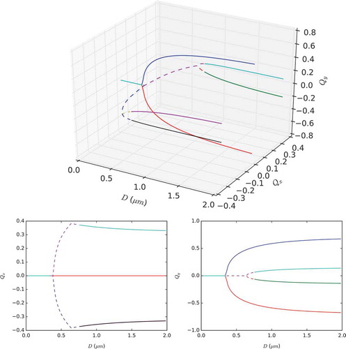
Figure 11. (Colour online) The deflation technique finds 81 equilibria for the LdG model at μm. Once rotational symmetries are discarded, 21 equilibria remain, which are depicted above ordered from left to right and top to bottom by the largest eigenvalue of the Jacobian of the RHS of Equations (4) and (5) (values of are given in Table 2). The first two equilibria are the diagonal and rotated solutions, with negative eigenvalues (i.e. stable), the remainder have positive eigenvalues (i.e. unstable). The equilibria are shown coloured by the order parameter s (blue at , increasing to red at ) and transparent white lines indicate the director direction n.

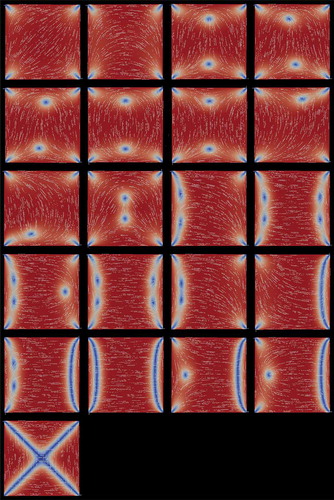
In the order presented in Figure 11, the 21 solutions can be classified into the following groups:

1. The first two panels show the familiar rotated and diagonal solutions, which have negative eigenvalues and are therefore stable. They have two splay vertices and two bend vertices each. Associating a topological charge of +1/4 to a splay vertex and a topological charge of – 1/4 to a bend vertex, it can be seen that the total topological charge is zero (the topological charge has to be zero in all cases).

2. In panels 3–5, we see the same number of splay and bend vertices and a pair of roughly aligned +1/2 and – 1/2 defects. These solutions (and all those in the following) have positive eigenvalues and are unstable.

3. In panels 6–7, we see four splay or four bend vertices accompanied by a pair of interior – 1/2 or +1/2 defects.

4. In panels 8–9, we see three splay (bend) vertices, one bend (splay) vertex and one −1/2 (+1/2) interior defect close to the bottom left vertex.

5. The solution in panel 10 has two splay and two bend vertices and a pair of +1/2 and – 1/2 defects close to the square centre, almost annihilating each other.

6. In panels 11–12 and 14–15, we see the two splay and two bend vertices along with a pair of +1/2 and – 1/2 defects localised along either one edge or a pair of opposite edges.

7. The 13th panel is slightly different. There is a pair of +1/2 and – 1/2 defects near the left edge and a + 1/2 defect near the right edge, neutralising the two corner bend defects of charge – 1/4 each. The remaining corners contain one splay and one bend defect.

8. In the remaining six panels (16–21), we see clear defect lines connecting the square vertices.

Lewis [37] analytically constructs nematic equilibria with interior defects on a square within the simpler continuum Oseen–Frank framework. We believe that there may be additional equilibria featured by a richer configuration of defects and whilst they are necessarily unstable, such equilibria can certainly be important for transient dynamics or may even be stabilised with external forces.

6. Discussion

We have numerically investigated off-lattice, lattice-based and continuum models for inhomogeneous nematic equilibria in square wells, subject to tangent Dirichlet boundary conditions. More specifically, we have studied the microscopic HGO and GB models, mesoscopic LL model and macroscopic LdG model for this confined system. Each approach provides different and complementary modelling perspectives. The off-lattice models are physically the most realistic with a large number of parameters that can be tuned to a wide variety of materials. Unlike LdG model, they do not fail near defects or near critical temperatures and can be used to probe critical phenomena. However, they are also the most computationally demanding with long simulation times, making it expensive to perform parameter sweeps with such models.

At the other end of the spectrum, it is easier to obtain stationary solutions for continuum PDE-based models such as LdG model, and thus these models are far more amenable to parameter sweeps. In addition, standard tools such as stability analysis are available and can provide further insights into solution properties. These models are widely used but their validity in extreme regimes, where geometrical and material length-scales become comparable (say on the nanometre scale when the domain size is comparable to the molecular size), is questionable. Lattice-based models offer an intermediate approach between the off-lattice and continuum approaches but they suppress the translational degrees of molecular freedom and are probably not effective in situations with fluid flow.

For nematics confined to square boxes as studied in this paper, both the off-lattice HGO and GB models fail to recover the familiar rotated solution. This is explained by the stability analysis in the LdG framework which clearly shows that the stable rotated solution branches only exist above a certain critical size, if the temperature and material constants are kept fixed. The square boxes in the HGO and GB simulations are smaller than this critical size and this is one explanation for the absence of the rotated solution in the off-lattice simulations. Since we do not have well-defined mappings between the GB parameters and the LdG elastic constants and temperature variable, it is difficult to make precise comparisons at this stage. A further feature is the clear difference in the order profiles of ‘splay’ and ‘bend’ vertices in the off-lattice models. This has not been picked up by either the lattice-based or continuum simulations. This could be a distinctive feature that is captured by the more realistic off-lattice models or the off-lattice models naturally correspond to materials with elastic anisotropy and hence, should be compared to LdG energies with elastic anisotropy or unequal material elastic constants, unlike the one-constant LdG energy used in this paper.

The LL simulations demonstrate a clear transition from a disordered state to the familiar diagonal and rotated solutions, induced by gradually decreasing the temperature. The GB stationary solution in Figure 4(b) is comparable to the third panel with in the LL simulations in Figure 7. On comparing the GB, LL and LdG simulations, we speculate that the models can be compared in the regimes specified by Figure 3(b), the third panel of Figure 7 and the first two rows of the right panel of Figure 7 for which all models converge to a solution which has reduced order near the centre of the square and has a constant eigenframe away from the centre. On comparing the HGO, LL and LdG simulations, we speculate that these models are comparable in the regimes specified by Figure 4(a), the fourth row of Figure 7 and the second row of the left panel in Figure 8. In future work, one could investigate these specific parameter regimes more exhaustively to understand the correspondences more closely.

We conclude this discussion by comparing the 2D WORS with the GB stationary pattern. The 2D WORS is a continuum LdG solution that is globally stable for small nanoscale wells (wells that are typically tens of nanometres in lateral dimension for prototype LC materials). The 2D WORS has a constant eigenframe everywhere on the square domain whereas the GB stationary solution has a constant eigenframe away from the centre of the square. Both solutions have a region of reduced order near the centre of the square and the GB stationary solution exhibits diagonal ordering within the region of reduced order. One could argue that the director profile in regions of low order is not of importance and since the GB and 2D WORS profiles match away from the centre, in regions of enhanced order, these are the same solutions. We further speculate that the constant eigenframe arises from the averaging of two different diagonal solutions in the GB or molecular framework. This does raise a natural question – are there truly molecular-level solutions with a constant eigenframe everywhere as the 2D WORS or is the 2D WORS a macroscopic approximation of the GB stationary solutions? It is equally possible that had we used different parameter values for the GB and LL simulations, we would recover a one-to-one correspondence with the 2D WORS, in the sense that we get a molecular-level solution with an approximately constant eigenframe everywhere inside the square domain. This numerical study raises several interesting questions about the relationships between molecular-level and continuum modelling, and we hope to pursue these questions in future work.

Disclosure statement

No potential conflict of interest was reported by the authors.

Additional information

Funding

This publication arises from research funded by the John Fell Oxford University Press (OUP) Research Fund (M.R., R.E.). R.E. would also like to thank the Royal Society for a University Research Fellowship. P.E.F. would like to acknowledge EPSRC grant EP/K030930/1, a Center of Excellence grant from the Research Council of Norway to the Center for Biomedical Computing at Simula Research Laboratory, project number 179578, and the generous support of Sir Michael Moritz and Harriet Heyman. A.M. is supported by an EPSRC Career Acceleration Fellowship EP/J001686/1 and EP/J001686/2. AM thanks the Mathematical Institute, University of Oxford for an OCIAM Visiting Fellowship which facilitated this collaboration.

References

- de Gennes PG, Prost J. The Physics of Liquid Crystals. New York (NY): Oxford University Press Inc.; 1974.
- Virga EG. Variational theories for liquid crystals. Vol. 8. London: Chapman & Hall; 1995.
- Berardi R, Lintuvuori JS, Wilson MR, et al. Phase diagram of the uniaxial and biaxial soft-core Gay-Berne model. J Chem Phys. 2011;135(13):134119.
- Care C, Cleaver D. Computer simulation of liquid crystals. Rep Prog Phys. 2005;68(11):2665–2700.
- Robinson M, Andrews SS, Erban R. Multiscale reaction-diffusion simulations with Smoldyn. Bioinfor- Matics. 2015;31(14):2406–2408.
- Erban R. Coupling all-atom molecular dynamics simulations of ions in water with Brownian dynamics. Proc R Soc A. 2016;472(2186):20150556.
- Tsakonas C, Davidson AJ, Brown CV, et al. Multistable alignment states in nematic liquid crystal filled wells. Appl Phys Lett. 2007;90(11):1913.
- Lewis AH, Garlea I, Alvarado J, et al. Colloidal liquid crystals in rectangular confinement: theory and experiment. Soft Matter. 2014;10(39):7865–7873.
- Luo C, Majumdar A, Erban R. Multistability in planar liquid crystal wells. Phys Rev E. 2012;85(6):061702.
- Kusumaatmaja H, Majumdar A. Free energy pathways of a multistable liquid crystal device. Soft Matter. 2015;11(24):4809–4817.
- Kralj S, Majumdar A. Order reconstruction patterns in nematic liquid crystal wells. Proc R Soc A. 2014;470(2169):20140276.
- Ladak S, Davidson A, Brown C, et al. Sidewall control of static azimuthal bistable nematic alignment states. J Phys D: Appl Phys. 2009;42(8):085114.
- Anquetil-Deck C, Cleaver DJ, Atherton TJ. Competing alignments of nematic liquid crystals on square- patterned substrates. Phys Rev E. 2012;86(4):041707.
- Davidson AJ, Mottram NJ. Conformal mapping techniques for the modelling of liquid crystal devices. Eur J Appl Math. 2012;23(01):99–119.
- Gˆarlea IC, Mulder BM. Defect structures mediate the isotropicnematic transition in strongly confined liquid crystals. Soft Matter. 2015;11(3):608–614.
- Slavinec M, Klemen EII, Ambro MDI, et al. Impact of nanoparticles on nematic ordering in square wells. Adv Cond Matter Phys. 2015;2015.
- Allen MP, Wilson MR. Computer simulation of liquid crystals. J Comput Aided Mol Des. 1989;3(4):335–353.
- Gay J, Berne B. Modification of the overlap potential to mimic a linear site–site potential. J Chem Phys. 1981;74(6):3316–3319.
- Lebwohl P, Lasher G. Nematic-liquid-crystal order–A Monte Carlo calculation. Phys Rev A. 1972;6(1):426–429.
- Erban R. From molecular dynamics to Brownian dynamics. Proc R Soc A. 2014;470(2167):20140036.
- Berne BJ. Gaussian model potentials for molecular interactions. J Chem Phys. 1972;56(8):4213.
- Berardi R, Emerson APJ, Zannoni C. Monte Carlo investigations of a Gay-Berne liquid crystal. J Chem Soc Faraday Trans. 1993;89(22):4069–4078.
- Luckhurst G, Simpson P. Computer simulation studies of anisotropic systems: VIII. the Lebwohl-Lasher model of nematogens revisited. Mol Phys. 1982;47(2):251–265.
- Chiccoli C, Pasini P, Zannoni C. A Monte Carlo simulation of the inhomogeneous Lebwohl-Lasher lattice model. Liq Cryst. 1987;2(1):39–54.
- Hastings WK. Monte Carlo sampling methods using Markov chains and their applications. Biometrika. 1970;57(1):97–109.
- Billeter J, Smondyrev A, Loriot G, et al. Phase-ordering dynamics of the Gay-Berne nematic liquid crystal. Phys Rev E. 1999;60(6):6831–6840.
- Majumdar A. Equilibrium order parameters of nematic liquid crystals in the Landau-de Gennes theory. Eur J Appl Math. 2010;21(02):181–203.
- Anquetil-Deck C, Cleaver D. Nematic liquid-crystal alignment on stripe-patterned substrates. Phys Rev E. 2010;82(3):031709.
- Logg A, Mardal KA, Wells GE. Automated solution of differential equations by the finite element method: the FEniCS book. Vol. 84. Springer Science & Business Media; 2012.
- Alnæs M, Blechta J, Hake J, et al. The FEniCS project version 1.5. Arch Numer Softw. 2015;3(100):9–23.
- Mottram NJ, Newton CJ Introduction to Q-tensor theory. arXiv preprint arXiv:14093542. 2014.
- Majumdar A, Milewski PA, Spicer A. Front propagation at the nematic-isotropic transition temperature. SIAM J Appl Math. 2016;76:1296–1320.
- Farrell PE, Beentjes CHL, Birkisson A The computation of disconnected bifurcation diagrams. 2016; arXiv:1603.00809 [math.NA].
- Keller HB. Numerical solution of bifurcation and nonlinear eigenvalue problems. In: Rabinowitz PH, editor. Applications of bifurcation theory. New York: Academic Press; 1977. p. 359–384.
- Farrell PE, Birkisson A, Funke SW. Deflation techniques for finding distinct solutions of nonlinear partial differential equations. SIAM J Sci Comput. 2015;37(4):A2026–A2045.
- Adler JH, Emerson DB, Farrell PE, et al. A deflation technique for detecting multiple liquid crystal equilibrium states. arXiv preprint arXiv:160107383. 2016.
- Lewis A. Defects in liquid crystals: mathematical and experimental studies [dissertation]. University of Oxford; 2016.