
ABSTRACT
Two top-down coarse-grained molecular simulation models for a chromonic liquid crystal, 3,6,7,10,11-hexa-(1,4,7-trioxa-octyl)-triphenylene, are tested. We use an extension of the well-known MARTINI model and develop a new coarse-grained model based on statistical associating fluid theory (SAFT)-γ perturbation theory. For both models, we demonstrate self-assembly in the isotropic phase of the chromonic and we test the effectiveness of both models in terms of the structures of the chromonic aggregates that are produced in solution and the thermodynamics of association. The latter is tested by calculations of the potential of mean force for dimers in solution, which measures the strength of molecular association. SAFT-γ provides valuable insights into the thermodynamics of assembly. Exploration of a range of interactions between unlike sites demonstrates that chromonic self-assembly only occurs in a small parameter space where the hydrophilic–lipophilic balance between aromatic core and ethylene oxide chains is optimal. Outside of this balance, chromonic self-assembly is replaced by the formation of conglomerates of molecules or short stacks.
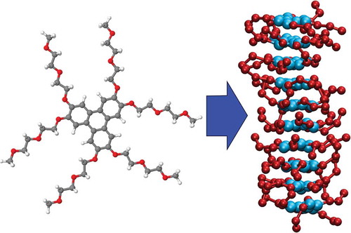
Graphical Abstract
1. Introduction
There has been considerable recent interest in chromonic liquid crystals. Chromonics are a non-conventional form of lyotropic liquid crystal [Citation1–Citation4]. Typically, chromonic mesogens are composed of a hydrophobic core (often a planar aromatic disc) with attached hydrophilic groups. This arrangement leads to molecules aggregating in aqueous solution to form stacks, which, at higher concentrations, self-organise to form lyotropic liquid crystal phases. Chromonic phases were initially found in groups of drug and dye molecules, with ionic functional groups providing the hydrophilic interactions [Citation5,Citation6]. However, there are also a small number of non-ionic chromonic molecules in which non-ionic groups, such as ethylene oxide chains, are sufficiently hydrophilic to provide the right hydrophobic–hydrophilic balance for aggregation in water without phase separation or crystallisation. An example is the well-known chromonic mesogen, 3,6,7,10,11-hexa-(1,4,7-trioxa-octyl)-triphenylene (TP6EO2M) [Citation7–Citation9], the structure of which is shown in . The recent increased interest in chromonic systems arises from potential applications in a range of areas including controllable self-assembly of gold nanorods [Citation10], biosensors [Citation11,Citation12] and as functional materials for fabricating highly ordered thin films [Citation13,Citation14].
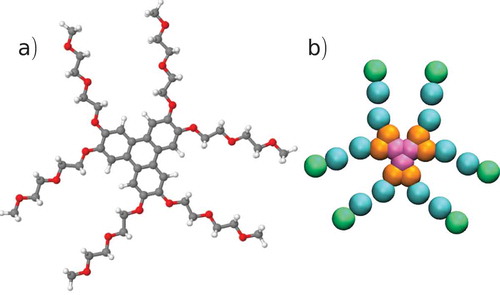
Figure 1. (Colour online) (a) Molecular structure of the chromonic liquid crystal, TP6EO2M. (b) Coarse-grained mapping used in this work, showing four bead types: CC – pink, CO – orange, AI – blue, AO – green.
From a simulation perspective, chromonic systems are extremely challenging. Self-assembly into stacks occurs over periods of tens or, in most cases, hundreds of nanoseconds. Moreover, formation of liquid crystal mesophases, by self-organisation of stacks, takes place over time scales that are considerably longer. In two recent studies, progress has been made in understanding and validating the structures expected in short chromonic stacks via long atomistic simulations [Citation15,Citation16]. There have also been previous attempts to produce coarse-grained models of chromonics. Chromonic self-assembly and phases have been seen in simple disc models [Citation17–Citation19] and, at longer length scales, dissipative particle dynamics studies have recently demonstrated the first full simulations of chromonic liquid crystal phase diagrams using up to 5000 mesogens in water [Citation20,Citation21].
However, there is a real challenge to produce coarse-grained models that capture the key structural features responsible for the local molecular packing within stacks and yet are computationally tractable, allowing longer time scale events to be seen. Such a model would provide a bridge between atom the valistic models and simple phenomenological models and would potentially shed light on many of the intriguing questions posed by chromonic self-assembly. For example, can simulations rationalise the architecture of complex stacks with multiple molecule cross-sections and/or unusual self-assembly behaviour [Citation22,Citation23], or can simulations unravel the structure of large aggregate structures, such as hollow cylinders [Citation24], which have been reported in some systems?
In this paper, we attempt to produce a new effective coarse-grained model for the chromonic mesogen, TP6EO2M, that bridges the gap between atomistic and highly coarse-grained simulation studies. Ideally, a new model should have chemical specificity so that results can be linked quantitatively to the system being studied. However, the model should also be sufficiently coarse-grained to allow for the simulation of large systems. In this study, we adapt the MARTINI force field, which was originally produced for lipids [Citation25] and peptides [Citation26] to act as a top-down coarse-grained force field for chromonic systems. Additionally, we attempt to develop a new top-down force field using statistical associating fluid theory (SAFT-γ) [Citation27], in which the coarse-grained nonbonded terms are obtained by fitting of thermodynamic data to produce generalised Lennard-Jones parameters (Mie potentials) to be used in molecular simulation.
2. Computational methods
2.1. MARTINI model
The coarse-grained MARTINI force field was originally developed for the simulation of lipids [Citation25] but has since been extended to other systems such as proteins [Citation26] and polymers [Citation28]. MARTINI consists of a number of distinct particle types, each of which represents a particular type of chemical group. These particles interact via Lennard-Jones 12:6 potentials, with the parameters used depending on the groups involved
with and
, for Lennard-Jones well depth
and distance parameter,
.
MARTINI is parametrised to reproduce the water/octanol partitioning free energies of a wide range of compounds. The mapping is usually four heavy atoms to one coarse-grained bead, although this has been altered for some particle types. Due to its relative ease of use and transferability, particularly compared to bottom-up coarse graining methods [Citation29,Citation30], MARTINI has been very widely used particularly in the simulation of biological systems. It has allowed simulations to reach higher time and length scales than fully atomistic models and usually provides qualitative or semi-quantitative accuracy for these systems.
Our initial coarse-grained model for TP6EO2M is based on the mapping shown in , which uses four types of coarse-grained sites: CC, CO, AI, AO plus water beads P4 and BP4. Each water bead represents four water molecules within a MARTINI simulation. As MARTINI is a 12:6 potential, and hence rather more repulsive at close distances than many coarse-grained water interactions, it does not have the liquid stability range of real water and is apt to freeze in contact with organic systems. Hence, as previously employed in many biological simulations, we use anti-freeze particles, BP4 sites, which interact in the same way with the TP6EO2M, as normal water cluster sites but which have a larger effective radius when interacting with normal water, P4 sites. (Without the anti-freeze particles, the presence of a chromonic stack is found to nucleate the freezing of MARTINI water.) The nonbonded interaction parameters for the model were taken from the MARTINI benzene and polyethylene oxide (PEO) models. In the original PEO model, each bead represents a single monomer. However, the hydrophilic arm in TP6EO2M is actually a methoxy group, and the mass of the end bead was altered to reflect this. In the benzene model, a bead represents a C2H2 unit; the mass of the beads in the aromatic core was therefore altered according to the number of hydrogen atoms associated with that bead. contains the Lennard-Jones parameters for the interactions in this system. Cross interactions were determined using the usual mixing rules: and
.
Table 1. MARTINI nonbonded parameters used in this study.
Bonds and angles were described by simple harmonic potentials, with bond lengths and angles taken from the energy minimised atomistic structure, mapped onto a coarse grained representation. Six improper dihedrals were required to keep the core of the molecule planar, but no other dihedral interactions were used in this model. The GROMACS topology file for the system is provided in the Supporting information. Bond interactions are used in preference to LINCS constraint bonds, as the highly interconnected nature of the core makes satisfying all of the constraints extremely difficult. Intramolecular interaction parameters are given in –.
Table 2. MARTINI angle parameters used in this study.
Table 3. MARTINI bond parameters used in this study.
Table 4. MARTINI improper dihedral parameters used in this study.
2.2. SAFT-γ model
The SAFT version used in this work is SAFT-γ Mie [Citation31], which is based on a version of SAFT suitable for potentials of variable range (SAFT-VR [Citation32]). The theory uses Mie (generalised Lennard-Jones) potentials as developed by Lafitte et al. [Citation33].
In the non-associating form of the theory, the Helmholtz free energy can be expressed as
where accounts for the ideal kinetic and translational energy contributions,
for the change in free energy due to attractive and repulsive interactions of the CG beads and
for the free energy contribution by forming chains.
The molecular model in the SAFT-γ Mie equation of state (EoS) is a chain of tangentially connected beads interacting through Mie potentials
with
where and
are, respectively, the well depth and the segment diameter,
and
are the repulsive and attractive exponents, for which
and
is the usual form of the Lennard-Jones potential.
We follow the strategy used by Müller, Jackson and co-workers for using SAFT to parameterise the nonbonded parts of a coarse-grained model [Citation34]. This has recently been successfully applied to lyotropic liquid crystal surfactants [Citation35]. The SAFT model for TP6EO2M was built by combining Mie potential parameters that were fitted to experimental vapour–liquid equilibria over a wide range of temperatures. The 3-bead benzene model by Lafitte et al. [Citation36] was used for the core beads and the PEO bead by Lobanova [Citation37] was used for the side chains. For the water beads, the coarse-grained biowater model by Lobanova et al. [Citation38] was used, which is optimised for the saturated-liquid density and surface tension at ambient conditions. Ref. [Citation37] also provides unlike interactions between the water and an EO bead, which were fitted to experimental excess enthalpies. However, in this work, we refitted all cross-interaction terms for our model, as described below, using the combining rules as a starting point to the fitting of Mie potentials to reproduce thermodynamic data.
The usual combining rules for contact distances give , for repulsive and attractive exponents [Citation33],
and well depth
Here, the parameter measures the extent of preferred interactions between species. For species that are chemically incompatible, for entropic or enthalpic reasons,
, and
for species where one group is well solvated by another.
In the current work, the EO–aromatic (EO–Ar) site interaction was fitted to 1,2-dimethoxyethane/benzene ((EO)2–benzene) enthalpies [Citation39,Citation40] of mixing with as the best fit. Aromatic–water (Ar–W) interactions were fitted to benzene–water liquid–liquid equilibrium compositions [Citation41–Citation43] with
as the best fit. EO–water (EO–W) interactions were fitted to triethylene glycol dimethyl ether/water ((EO)4–W) enthalpies of mixing [Citation44,Citation45] with
as the best fit. Thus, interactions involving EO are more attractive (EO–Ar, EO–W) than the combining rules suggest, while the Ar–W interaction is considerably less attractive than the combining rule predicts. The solubility and excess enthalpy calculations of the SAFT models were performed using the SAFT-γ Mie EoS and numerical solvers provided by the gSAFT package (Process Systems Enterprise Ltd. [Citation46]).
The Mie potentials () were used as nonbonded interactions in the MD simulations, in combination with intramolecular parameters derived from the MARTINI force field. In our initial SAFT model, the values obtained from nonbonded potentials were used as equilibrium bond lengths (in the spirit of the SAFT theory which uses tangentially bonded spheres) in combination with the same force constants used in the MARTINI model. The angle potentials used were identical to the MARTINI model. The same improper dihedral potentials were also used in the SAFT model, but with a five times stronger (150 kJ mol−1) force constant to keep the core planar. In a later development of the SAFT model, we used the same bond lengths as used in MARTINI, in combination with SAFT nonbonded parameters.
Table 5. SAFT nonbonded parameters used in this study.
2.3. Coarse-grained simulations
All molecular dynamics simulations were carried out using GROMACS 4.6.7. The equations of motion were solved using the leap-frog integrator with a time step of 2 fs (MARTINI) and 5 fs (SAFT). All simulations were carried out at a temperature of 280 K and a pressure of 1 bar, using the Nosé–Hoover thermostat and the Parrinello–Rahman barostat. The van der Waals, neighbour list and coulomb cut-offs were set to 1.2 nm (MARTINI) and 1.5 nm (SAFT). Simulations of a stacked MARTINI configuration were prepared by initially creating a stack of 10 TP6EO2M molecules, and solvating with 4709 water beads and 523 antifreeze beads. An energy minimisation was carried out, and the structure was equilibrated for 400 ps in the constant-NVT ensemble. A production run was then carried out in the constant-NPT ensemble for 100 ns.
MARTINI simulations were also carried out from a dispersed starting configuration. Ten TP6EO2M molecules were placed randomly in a simulation box and solvated with 3917 water beads and 435 antifreeze beads. The energy of the system was minimised, and a 10-ns equilibration run was carried out in the NVT ensemble. A 100-ns production was then carried out in the NPT ensemble.
For the SAFT-γ simulations, a randomly generated vapour configuration of 10 TP6EO2M molecules and 16,740 water beads was prepared. The system was compressed at 500 bar and 450 K for 1000 ps and equilibrated at 280 K and 1 bar for 500 ps using the Berendsen thermostat and Berendsen barostat in the NPT ensemble. A production run was carried out of at least 100 ns with the Nosé–Hoover thermostat and the Parrinello–Rahman barostat.
2.4. Potential of mean force calculations
The potential of mean force (PMF) for a TP6EO2M dimer was calculated by constraining the separation distance between the centres of mass (COMs) of the cores of two TP6EO2M molecules at a range of distances from 0.35 to 2.35 nm and calculating the average constraint force, . For each distance,
was calculated by integrating over the separation distance, using:
where is Boltzmann’s constant and T is the temperature.
First, a dimer was placed in a simulation box with 6914 water beads and 798 antifreeze beads, and the structure was energy minimised. The system was equilibrated in the constant-NPT ensemble for 1 ns with the Berendsen thermostat and barostat, followed by 5 ns with the Nosé–Hoover thermostat and the Parrinello–Rahman barostat. A further 5-ns constant-NVT equilibration was carried out at the equilibrium density from the constant-NPT simulations. An initial pull simulation was carried out, with the distance between the COMs of the aromatic cores of the two molecules constrained and increased from 0.35 nm at a rate of 0.01 nm ps−1. Frames were then selected from this simulation at a range of distances, clustered more closely around the expected energy minimum. At each of these distances, a 25-ns simulation was carried out with COM–COM distance constrained, the last 20 ns of which was used to generate data for the PMF calculation.
3. Results
3.1. MARTINI model
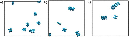
shows a series of snapshots taken from an initially dispersed TP6EO2M system in water. The system spontaneously self-assembles over time to form short chromonic stacks, with aggregates (H-aggregates) growing through addition of a monomer or merging of two short stacks. If a stack is pre-assembled and solvated, it is stable for long simulation times (>100 ns). An equilibrated self-assembled stack shows the same structure as that seen atomistically for TP6EO2M, with the molecules exhibiting liquid crystalline, rather than crystalline, order.
Figure 2. (Colour online) A series of snapshots taken from the simulation of the MARTINI model of TP6EO2M in water at 280 K, showing the central aromatic core of molecules, taken at (a) the start of the simulation, (b) 50 ns and (c) 90 ns. The simulation trajectory shows the spontaneous self-assembly of short chromonic stacks.
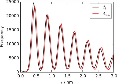
Two distinct measures of the distance between two molecules in a stack have been used in previous studies of TP6EO2M. The first, , is simply the distance between the COMs of two molecules, while the stacking distance,
, is the distance between the molecules projected along the average of the vectors normal to the cores of the two molecules. Probability distributions for the two distances are shown in . The maximum of the peak
for adjacent molecules is 0.42 nm. The distribution for
is shifted so that the maximum is at 0.46 nm. This reflects the fact that there is a slight offset between molecules in the stack. This stacking demonstrates H-aggregation, rather than J-aggregation. The latter would have a larger systematic offset. It is noted that the peaks do not have a long tail at higher distances, as there are no distinct bends in the stack. As expected, the stacking distances between molecules are close to the contact distance of the MARTINI nonbonded potentials for the CG sites. These separations are the minimum possible for this model due to the size of beads used but are (of course) slightly larger than the experimental and atomistic value of
, which correspond to the distance of separation for single aromatic carbon atoms.
Figure 3. (Colour online) Probability distributions for the pair distances, , and
for a single chromonic stack simulated at 280 K using the MARTINI model for TP6EO2M.
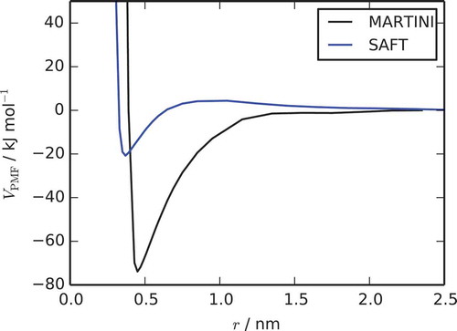
The PMF for the separation of a TP6EO2M dimer is given in . The PMF has a similar shape to that reported for the atomistic system by Akinshina et al., with a short range repulsive and a long range attractive part. The free energy of association, , for the formation of a dimer can be obtained from the maximum well depth of the PMF. For this model, ΔG = −73.9 ± 1.5 kJ mol−1 at a concentration of
, which is higher than the value of −40.7 ± 1.4 kJ mol−1 for a PMF obtained for the atomistic system. Therefore, the MARTINI model provides only semi-quantitative thermodynamic data.
Figure 4. (Colour online) Potential of mean force curves calculated for the separation of a dimer of two molecules for the MARTINI model and the SAFT-γ model.
We note that coarse graining, as desired, allows for a huge speed-up in observing chromonic assembly, with savings arising from a faster exploration of phase space in addition to a large reduction in the number of sites simulated. TP6EO2M reduces from 138 sites to 27 (a factor of and four water molecules (12 sites) reduce to 1 site.
3.2. SAFT-γ model
Using the initial SAFT-γ model developed above, which includes fitted cross-interactions, we see chromonic stacking, as seen in the MARTINI model. Molecular spacings in a stack are corresponding to the smaller coarse-grained sites arising in SAFT-γ. It is interesting to note that if instead of fitted cross-interactions, we use instead interactions generated by standard combining rules for Lennard-Jones interactions, then SAFT-γ TP6EO2M molecules are perfectly soluble in water, with no association over
. Association into chromonic stacks therefore arises when there are less favourable interactions between aromatic groups and water. Noting that part of this unfavourable interaction includes the hydrophobic interaction from release of water when aromatic groups interact, which is incorporated into the nonbonded interaction parameters within a coarse-grained model.
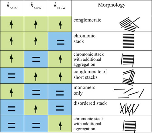
To investigate this further, we looked at a range of SAFT-γ models, as shown in . For these models, we consider only combination of cases where or 0.0. The former value corresponds to unfavourable interactions relative to the combining rules. Here, as shown in , a range of different aggregation behaviour is possible, from no aggregation where molecules are perfectly soluble, to conventional chromonic stacking, to effective phase separation with formation of non-equilibrium conglomerates of molecules or short stacks.
Figure 5. (Colour online) The influence of unfavourable cross-interactions on chromonic stacking. Up arrows indicate interactions that are less favourable than mixing rules with . Equal signs indicate
. Chromonic stacks are found when aromatic group interactions with both ethylene oxide and water are unfavourable, apart from when ethylene oxide and water interactions are also unfavourable.
In SAFT, equilibrium bond lengths, , between coarse-grained sites are usually set to the same value as
for a given pair of atom types. This means that while the bulk properties are correct, the internal structure is less faithful to an underlying atomistic framework. If SAFT is used to generate parameters for a simple polymer or oligomer chain or used for a simple linear surfactant, this is unlikely to be a problematic. However, for TP6EO2M, we noted the presence of some configurations where a dimer was able to sample the arrangement shown in . We particularly noted this in PMF calculations, when the core–core distance was constrained to relatively small distances. The structure seen here is unphysical and can be attributed to the relatively large
ratio. To eliminate these configurations, we took the fitted SAFT model and further modified it to use the same bond lengths as used in the MARTINI model. After this modification, the interdigitated structure of was no longer observed (see Supplementary data).
Figure 6. (Colour online) Simulation snapshot of a dimer using the original SAFT model with unadjusted bond lengths, with the core–core distance constrained at 0.55 nm. Only the aromatic cores are shown.

The PMF generated with this final SAFT model is shown in . As with MARTINI, a deep attractive potential well is seen, which is responsible for spontaneous aggregation in solution. The slight net repulsion seen at longer COM distances reflects the slight preference for EO groups to be fully solvated in water rather than to be in contact with each other. In contrast to MARTINI, SAFT underestimates the free energy of association. It is possible that improvements to the SAFT well-depth may be possible if appropriate free energies were available for fitting of ethylene oxide cross-interaction terms (see Section 4), and also if we were able to move to the fitting of free energies for the interaction of extended aromatic systems instead of benzene.
4. Discussion
At first glance, the non-ionic chromonic system, TP6EO2M, appears to be quite a simple system to model, i.e. representable by two types of Lennard-Jones beads. However, the simplicity of the chemical structure hides a wealth of subtle complexities arising from modelling the right hydrophilic–lipophilic balance within different parts of the molecule. The initial clue to the complexity lies in the earlier atomistic simulation work of Akinshina et al. [Citation16]. In this paper, it was shown that the contribution to association-free energy arises from both entropic and enthalpic contributions and these are similar in magnitude ( and
to
). Favourable enthalpic interactions arise when discs self-assemble but there is also a strong hydrophobic interaction arising from the release of solvent. Moreover, the balance of interactions between chains and solvent, and between aromatic cores and solvent, is also important. For example, changing the atomistic force field from OPLS to GAFF leads to reduced hydration of ethylene oxide chains and consequently to association which is too strong to lead to the formation of fully hydrated chromonic stacks.
In this coarse-grained study, the same balance of interactions is found to be absolutely crucial. Moreover, within a coarse-grained representation, the coarse-graining procedure changes the balance between enthalpic and entropic interactions. Coarse-grained water has a lower gain in entropy, in comparison with real water, when freed from interaction with a chromonic molecule. Consequently, the free energy balance within a coarse-grained model must be represented by more favourable enthalpic interactions favouring association. One initial consequence of this observation is that in coarse graining, matching enthalpic interactions to an atomistic reference in a chromonic (or related) system is going to lead to poorer thermodynamics than if free-energies are used in the coarse-graining procedure. We note also the early work of Klein and co-workers who used transfer free energies as part of the development of early successful coarse-grained surfactant models [Citation47].
The reason for the simple MARTINI model being successful, in terms of capturing chromonic assembly, is therefore very apparent. The nonbonded interactions within MARTINI are designed to model the partitioning (and hence the transfer free energy) from water to octanol. MARTINI is therefore able to do a reasonably good job of capturing both the overall hydrophilic–lipophilic balance for a chromonic molecule in water, and the relative hydrophilic–lipophilic balance between the different parts of the molecule.
Coarse graining using SAFT-γ provides further insights. shows that across a small parameter range for the unlike interactions, one can achieve a range of aggregation behaviour, with chromonic self-assembly only occurring at the right balance of hydrophilic and lipophilic interactions for the aromatic and ethylene oxide components. If the balance of interactions is wrong, the self-assembly process may not be observed within a reasonable simulation time, either due to a lack of self-assembly, or the formation of other conglomerates.
The ability of the SAFT-γ procedure to fit to free energy, enthalpy, entropy and free-energy dependent data provides a powerful mechanism to match the correct hydrophilic–lipophilic balance. To ensure a correct balance, free energy (or free-energy dependent) experimental data have to be available for all interactions of interest. For the SAFT-γ model in this work, we have used free energy and free-energy dependent data for four out of six interactions (one out of three unlike interactions), while for the water–ethylene oxide and the aromatic–ethylene oxide interactions, we have used enthalpies of mixing due to lack of other experimental data. The shortcomings of the SAFT-γ are at least partially attributed to not ensuring the correct entropic contributions in those two ethylene oxide interactions.
We have also highlighted another weakness to the SAFT-γ approach to coarse-graining. In order to obtain an accurate structure for the TP6EO2M molecule, we manually changed the bond lengths to match the atomistic structure. While successful for a dimer or stack system solvated with water, this approach would be likely to cause issues if dealing with a bulk system, because the model has been parametrised to match bulk quantities, such as densities, on the basis that and
are equal. This suggests that the current ability to construct models for complex chemical systems with SAFT-γ is limited by its structural accuracy, and this is something that must be addressed in future work. Moreover, for complex chemical structures, such as TP6EO2M, a small contribution to the balance of hydrophilic/hydrophobic/lipophilic interactions arises from the parts of configurational space that are accessible (or inaccessible) in a dimer interaction. In this example, the accessible configurational space can be modified by the bond lengths used in representing complex structures.
Finally, it is worth commenting on a comparison of the methodologies adopted here and alternative bottom-up strategies, which rely on a fit to an underlying atomistic reference system. The two most commonly used bottom-up methods are the multi-scale coarse-grained (MS-CG) method of Voth and co-workers [Citation48–Citation50] (often referred to as force matching) and the iterative Boltzmann inversion (IBI) method [Citation51]. IBI potentials are traditionally fitted to reproduce distribution functions in the atomistic reference system, so would be able to reproduce the structure of a chromonic stack given that structure within an atomistic system. However, good fitting is difficult to achieve in IBI when there are multiple partial radial distribution functions (RDFs) to fit arising from cross-interactions. Moreover, for systems such as this, the reproduction of thermodynamic quantities, particularly association free energies, tends to be poor, and it is unlikely that the same IBI model can reproduce both the correct structure of a chromonic stack and the correct self-assembly behaviour seen in dilute solution. The MS-CG method is, in principle, easier to fit to an atomistic reference system for a chromonic than multiple partial RDFs. However, here transferability between different concentrations and/or different aggregate states would be expected to be rather poor. In addition, as with IBI, there is no strong expectation that the thermodynamics of assembly, seen to be so crucial in the current study, could be easily reproduced.
In preliminary work, we have tested the MS-CG approach for the TP6EO2M/water system using an underlying atomistic reference composed of dispersed monomers, dimers and trimer stacks, solvated with water. This reference was chosen due to the tightly bound nature of the molecules in a chromonic stack, which led to poor sampling of the forces between atoms for many distances and orientations. The MS-CG scheme does not necessarily guarantee that the CG model will recover the reference atomistic structure, due to the assumptions made in trying to map all of the interactions in the atomistic system onto two-body coarse grained potentials. In practice, we found that using this MS-CG model, TP6EO2M tends to induce crystallisation of the CG water, so the correct aggregation behaviour is not seen. Running CG simulations without water, using the same MS-CG force field, led to the rapid collapse of a stacked starting configuration into a disordered conglomerate.
Hence, the modelling methods suggested in the present study currently seem to be the best realistic approach for designing coarse-grained models of chromonic systems when it is necessary to capture specific molecular interactions.
5. Conclusions
We have successfully produced two coarse-grained models to study molecular association in the non-ionic chromonic TP6EO2M/water system. The MARTINI model, extended to chromonics, is shown to work well in modelling self-assembly in solution, giving reasonably good PMF interactions for molecular association. In this model, considerable speed-ups are accessible in comparison to atomistic models. These are achieved via a considerable reduction in the number of interaction sites for the coarse-grained model: a reduction in sites of is achieved, depending on system size and concentrations, leading to a dramatic reduction in pair interactions
. Second, a speed-up in dynamics occurs as coarse-grained models move more quickly through phase space than their atomistic counterparts.
We show also that SAFT-γ perturbation theory provides a powerful methodology to carry out coarse-graining of the intermolecular interactions. We are able to use SAFT-γ fitting to experimental data to produce a coarse-grained model to describe TP6EO2M self-assembly in water. SAFT provides molecular insight into the nature of the interactions which are responsible for chromonic phase behaviour. Moreover, we see that the correct hydrophilic–lipophilic balance is absolutely crucial for chromonic association to take place in water, and this statement applies to the interactions of component parts of a chromonic molecule within water, in addition to the molecule as a whole.
In future, we suggest that the coarse-graining approaches we use here, which are both fast and effective, could be used for screening molecules for chromonic behaviour and designing new chromonic systems with desired self-assembly behaviour.
Acknowledgements
The authors would like to acknowledge the support of the Engineering and Physical Sciences Research Council (EPSRC) in the United Kingdom: [Grant Number EP/J004413/1] and Durham University for the use of its HPC facility, Hamilton. TDP would like to thank EPSRC for the award of a studentship. The authors would like to thank PSE Ltd. for the use of its numerical solvers provided by the gSAFT package.
Disclosure statement
No potential conflict of interest was reported by the authors.
Supplemental data
Supplemental data for this article can be accessed here.
Additional information
Funding
References
- Lydon J. Chromonic liquid crystalline phases. Liq Cryst. 2011;38(11–12):1663–1681.
- Lydon J. Chromonic review. J Mater Chem. 2010;20(45):10071–10099.
- Lydon J. Chromonic mesophases. Curr Opin Colloid Interface Sci. 2004;8(6):480–490.
- Lydon J. Chromonic liquid crystal phases. Curr Opin Colloid Interface Sci. 1998;3(5):458–466.
- Sandqvist H. Anisotropic aqueous solution. Ber Dtsch Chem Ges. 1915;48:2054–2055.
- Hartshorne NH, Woodard GD. Mesomorphism in the system disodium chromoglycate-water. Mol Cryst Liq Cryst. 1973;23(3–4):343–368.
- Boden N, Bushby R, Hardy C, et al. Phase behaviour and structure of a non-ionic discoidal amphiphile in water. Chem Phys Lett. 1986;123(5):359–364.
- Boden N, Bushby R, Hardy C. New mesophases formed by water soluble discoidal amphiphiles. J Physique Lett. 1985;46(7):325–328.
- Boden N, Bushby RJ, Ferris L, et al. Designing new lyotropic amphiphilic mesogens to optimize the stability of nematic phases. Liq Cryst. 1986;1(2):109–125.
- Park HS, Agarwal A, Kotov NA, et al. Controllable side-by-side and end-to-end assembly of Au nanorods by lyotropic chromonic materials. Langmuir. 2008;24(24):13833–13837.
- Shiyanovskii SV, Schneider T, Smalyukh II, et al. Real-time microbe detection based on director distortions around growing immune complexes in lyotropic chromonic liquid crystals. Phys Rev E. 2005;71(2):20702.
- Shiyanovskii SV, Lavrentovich OD, Schneider T, et al. Lyotropic chromonic liquid crystals for biological sensing applications. Mol Cryst Liq Cryst. 2005;434:587–598.
- Kaznatcheev KV, Dudin P, Lavrentovich OD, et al. X-ray microscopy study of chromonic liquid crystal dry film texture. Phys Rev E. 2007;76(6):61703.
- Olivier Y, Muccioli L, Lemaur V, et al. Theoretical characterization of the structural and hole transport dynamics in liquid-crystalline phthalocyanine stacks. J Phys Chem B. 2009;113(43):14102–14111.
- Chami F, Wilson MR. Molecular order in a chromonic liquid crystal: a molecular simulation study of the anionic azo dye sunset yellow. J Am Chem Soc. 2010;132(22):7794–7802.
- Akinshina A, Walker M, Wilson MR, et al. Thermodynamics of the self-assembly of non-ionic chromonic molecules using atomistic simulations. The case of TP6EO2M in aqueous solution. Soft Matter. 2015;11(4):680–691.
- Edwards RG, Henderson JR, Pinning RL. Simulation of self-assembly and lyotropic liquid-crystal phases in model discotic solutions. Mol Phys. 1995;86(4):567–598.
- Al-Lawati ZH, Alkhairalla B, Bramble JP, et al. Alignment of discotic lyotropic liquid crystals at hydrophobic and hydrophilic self-assembled monolayers. J Phys Chem C. 2012;116(23):12627–12635.
- Maiti P, Lansac Y, Glaser M, et al. Isodesmic self-assembly in lyotropic chromonic systems. Liq Cryst. 2002;29(5):619–626.
- Walker M, Masters AJ, Wilson MR. Self-assembly and mesophase formation in a non-ionic chromonic liquid crystal system: insights from dissipative particle dynamics simulations. Phys Chem Chem Phys. 2014;16(42):23074–23081.
- Walker M, Wilson MR. Formation of complex self-assembled aggregates in non-ionic chromonics: dimer and trimer columns, layer structures and spontaneous chirality. Soft Matter. 2016;12:8588–8594.
- Collings PJ, Goldstein JN, Hamilton EJ, et al. The nature of the assembly process in chromonic liquid crystals. Liq Cryst Rev. 2015;3(1):1–27.
- Mercado BR, Nieser KJ, Collings PJ. Cooperativity of the assembly process in a low concentration chromonic liquid crystal. J Phys Chem B. 2014;118(46):13312–13320.
- Berlepsch H, Ludwig K, Böttcher C. Pinacyanol chloride forms mesoscopic H-and J-aggregates in aqueous solution–a spectroscopic and cryo-transmission electron microscopy study. Phys Chem Chem Phys. 2014;16(22):10659–10668.
- Marrink S, Risselada HJ, Yefimov S, et al. The MARTINI force field. J Phys Chem B. 2007;111(27):7812.
- Monticelli L, Kandasamy SK, Periole X, et al. The MARTINI coarse-grained force field: extension to proteins. J Chem Theory Comput. 2008;4(5):819–834.
- Lymperiadis A, Adjiman CS, Galindo A, et al. A group contribution method for associating chain molecules based on the statistical associating fluid theory (SAFT-). J Chem Phys. 2007;127(23):234903.
- Nawaz S, Carbone P. Coarse-graining poly(ethylene oxide)–poly(propylene oxide)–poly(ethylene oxide) (PEO–PPO–PEO) block copolymers using the MARTINI force field. J Phys Chem B. 2014;118(6):1648–1659.
- Peter C, Kremer K. Multiscale simulation of soft matter systems. Faraday Discuss. 2010;144:9–24.
- Peter C, Kremer K. Multiscale simulation of soft matter systems – from the atomistic to the coarse-grained level and back. Soft Matter. 2009;5(22):4357.
- Papaioannou V, Lafitte T, Avendaño C, et al. Group contribution methodology based on the statistical associating fluid theory for heteronuclear molecules formed from Mie segments. Journal of Chemical Physics. 2014;140(5):054107.
- Gil-Villegas A, Galindo A, Whitehead PJ, et al. Statistical associating fluid theory for chain molecules with attractive potentials of variable range. J Chem Phys. 1997;106(10):4168–4186.
- Lafitte T, Apostolakou A, Avendaño C, et al. Accurate statistical associating fluid theory for chain molecules formed from Mie segments. J Chem Phys. 2013;139(15):154504.
- Müller EA, Jackson G. Force-field parameters from the SAFT- equation of state for use in coarse-grained molecular simulations. Ann Rev Chem Biomolec Eng. 2014;5:405–427.
- Herdes C, Santiso EE, James C, et al. Modelling the interfacial behaviour of dilute light-switching surfactant solutions. J Colloid Interface Sci. 2015;445:16–23.
- Lafitte T, Avendaño C, Papaioannou V, et al. SAFT- force field for the simulation of molecular fluids: 3. Coarse-grained models of benzene and hetero-group models of n-decylbenzene. Mol Phys. 2012;110(11–12):1189–1203.
- Lobanova O Development of coarse-grained force fields from a molecular based equation of state for thermodynamic and structural properties of complex fluids [dissertation]. Imperial College London; 2014.
- Lobanova O, Avendano C, Lafitte T, et al. SAFT- force field for the simulation of molecular fluids: 4. A single-site coarse-grained model of water applicable over a wide temperature range. Mol Phys. 2015;113(9–10):1228–1249.
- Koldobskaya LL, Gaile AA, Semenov L, et al. Enthalpy of Mixing of Hydrocarbons with Oxygen and Nitrogen Containing Polar Solvents. Deposited Doc. VINITI. 1987. p. 1–17.
- Kehiaian H, Sosnkows H. Enthalpy of mixing of ethers with hydrocarbons at 25 degrees c and its analysis in terms of molecular surface interactions. J Chim Phys-Chim Biol. 1971;68(6):922–934.
- Bittrich H, Gedan H, Feix G. Influencing the solubility of hydrocarbons in water. Z Phys Chem Leipzig. 1979;260(5):1009–1013.
- Moule DC, Thurston WMA. Method for the determination of water in nonpolar liquids; the solubility of water in benzene. Can J Chem. 1966 Jun;44(12):1361–1367.
- Tare J, Thurston S, Kher M. Indian Chem. Eng. studies in ternary phase (liquid) equilibrium. 1976;18(4):27–30.
- Burgdorf R. oCLC: 75622577. Untersuchungen thermophysikalischer Eigenschaften ausgewählter organischer Flüssigkeitsgemische. Als ms. gedr ed. Berichte aus der Verfahrenstechnik:Aachen:Shaker;1995.
- Dohnal V, Roux AH, Hynek V. Limiting partial molar excess enthalpies by flow calorimetry: some organic solvents in water. J Solution Chem. 1994 Aug;23(8):889–900.
- gSAFT Advanced Thermodynamics, https://www.psenterprise.com/products/gsaft/. 2017. [Cited 2017 Mar 20].
- Shinoda W, DeVane R, Klein ML. Multi-property fitting and parameterization of a coarse grained model for aqueous surfactants. Mol Simul. 2007;33(1–2):27–36.
- Izvekov S, Voth GA. A multiscale coarse-graining method for biomolecular systems. J Phys Chem B. 2005;109(7):2469–2473.
- Izvekov S, Violi A, Voth GA. Systematic coarse-graining of nanoparticle interactions in molecular dynamics simulation. J Phys Chem B. 2005;109(36):17019–17024.
- Noid W, Chu JW, Ayton GS, et al. Multiscale coarse-graining and structural correlations: connections to liquid state theory. J Phys Chem B. 2007;111(16):4116–4127.
- Reith D, Pütz M, Müller-Plathe F. Deriving effective mesoscale potentials from atomistic simulations. J Comput Chem. 2003;24(13):1624–1636.