Considerations in the determination of orientational order parameters from X-ray scattering experiments

ABSTRACT

An assessment of the data processing and analysis methods used to obtain the second- and fourth-rank orientational order parameters of liquid crystals from X-ray scattering experiments has been carried out, using experimental data from four extensively studied alkyl-cyanobiphenyls and calculated data generated from two general types of theoretical orientational distribution function. The application of a background subtraction and two different baseline correction methods to the scattering profiles is assessed, along with three different methods to analyse the processed data. The choice of baseline correction method is shown to have a significant effect: an offset to zero overestimates the order parameters from the experimental and calculated data sets, particularly for lower order parameters arising from broad distributions, whereas an offset to a value estimated from regions of low scattering intensity provides experimental values close to those reported from other experimental techniques. By contrast, the three different analysis methods are shown generally to result in relatively small absolute differences between the order parameters. We outline a straightforward general approach to experimental X-ray scattering data processing and analysis for uniaxial phases that results in order parameters that match well with those reported using other experimental techniques.

Graphical Abstract

KEYWORDS:

• X-ray scattering
• order parameter
• background subtraction
• baseline offset
• nematic
• orientational distribution
• alkyl-cyanobiphenyl

1. Introduction

The use of X-ray scattering experiments to probe the structure of materials has proven invaluable in many areas of science over the course of many decades, and the study of liquid crystals is no exception. X-ray studies of liquid crystal phases provide a wealth of information relating to the structure of different mesophases, manifesting as the numbers, positions, and intensities of peaks in the detected scattering patterns. The nematic phase constitutes the simplest of the liquid crystal phases, typically resulting in just two sets of primary scattering peaks for phases comprising rod-like (calamitic) molecules: one set of small-angle peaks relating to the average periodicity of electron density along the director, and one set of wide-angle peaks relating to the average periodicity of electron density orthogonal to the director [1]. In a sample exhibiting no bulk alignment, these peaks are observed in a 2D X-ray scattering experiment as rings, but in a bulk-aligned sample, the small-angle peaks are observed parallel to the director and the wide-angle peaks are observed perpendicular to the director, as shown in a schematic diagram of an experimental X-ray scattering experiment in Figure 1.

Figure 1. (Colour online) Schematic representation of an experimental X-ray scattering experiment for magnetically aligned nematic samples.

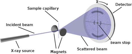
The intensity of the wide-angle peaks around the angle χ (labelled in Figure 1) relates to the degree of ordering of the liquid crystal sample, and a particular advantage of X-ray scattering is that, in principle, it is a method that enables determination of the full orientational distribution function, f(β), of a uniaxial phase, where β is the angle made between the principal axis of a molecule and the average orientation of all the principal molecular axes, termed the director, n. This distribution function is typically expanded as a sum of the even Legendre polynomials, P_L(cosβ), given by Equation (1), in which the coefficients, f_L, are defined by Equation (2), where the values of ⟨P_L⟩ are commonly termed the orientational order parameters of a liquid crystal phase [2,3]. For a known distribution function, the orientational order parameters may be determined using Equation (3) [2,3].

(1) $f\left(\beta \right)=\sum _L{f}_L{P}_L\left(cos\beta \right);(L\mathrm{e}\mathrm{v}\mathrm{e}\mathrm{n})$(1)

(2) $f_L=\left(\frac{2L+1}{2}\right)⟨P_L⟩$(2)

(3) $⟨P_L⟩=\frac{\underset{0}{\overset{\pi }{\int }}f\left(\beta \right)P_L\left(cos\beta \right)sin\beta \mathrm{d}\beta }{\underset{0}{\overset{\pi }{\int }}f\left(\beta \right)sin\beta \mathrm{d}\beta }$(3)

The ability of X-ray scattering experiments, in principle, to determine many or all of the order parameters is extremely desirable, particularly when compared with many other methods, such as UV-visible or IR absorbance measurements and NMR experiments that are typically restricted to determining the second-rank order parameter, ⟨P₂⟩ [4], and Raman scattering or fluorescence depolarisation measurements that are typically restricted to determining only ⟨P₂⟩ and ⟨P₄⟩ [5–7]. The measurement of ⟨P₂⟩, ⟨P₄⟩ and ⟨P₆⟩ from electron paramagnetic resonance (EPR) experiments has been reported [8], but this technique is limited to the detection of spin probes, from which the ordering of the liquid-crystalline material must be inferred. As a result, the determination of orientational order parameters from X-ray scattering experiments has been the subject of many studies in a wide range of fields, such as the study of membrane structures [9], polymers [10], elastomers [11], and nanoparticle systems [12].

The behaviour of typical nematic phases has been shown to be broadly consistent with Maier–Saupe theory [13], for which the different order parameters have a consistent relationship, enabling the distribution function f(β) (peaked at β = 0) to be inferred reliably from a single value of ⟨P₂⟩. However, some phases do not exhibit behaviour consistent with such distribution functions, such as the twist-bend (TB) phase, which is reported to exhibit a heliconical structure [14,15], and the de Vries smectic A phase, which is proposed to exhibit a sugar-loaf or diffuse-cone (volcano) distribution function [16–19], in which the maximum probability of molecular orientations is not necessarily at β = 0. Measurements of ⟨P_L⟩ values for L ≥ 2 are required to study systems with such distribution functions, and reliable techniques for determining these values are highly desirable since a maximum entropy argument [3,13] can be used to infer an orientational distribution function from measured values of ⟨P_n⟩.

Despite the capability of X-ray scattering experiments in principle, a particular difficulty in determining the orientational distribution function of a sample from X-ray scattering data is that of relating the molecular orientational distribution to the orientational dependence of the intensity of the wide-angle scattering peaks, I(χ), because the transformation relies on a number of assumptions.

In the field of liquid crystals, a widely used set of assumptions originally proposed by Leadbetter et al. were based on uniaxial molecular symmetry, and on the scattering occurring from clusters of uniformly aligned interfering particles (molecules) [20–23]. The application of these assumptions resulted in the derivation of Equation (4), which relates the χ-dependence of the integrated wide-angle intensity profile directly to the orientational distribution function, f(β), of the clusters of molecules in the ordered mesophase [20,23].

(4) $I\left(\chi \right)=\underset{\beta =\chi }{\overset{\pi /2}{\int }}\frac{f\left(\beta \right)sin\beta }{{cos}^2\chi \sqrt{{tan}^2\beta -{tan}^2\chi }}\mathrm{d}\beta$(4)

This expression readily enables the order parameters, ⟨P_L⟩, to be determined from the integrated intensity of the wide-angle X-ray peaks, the method for which is described fully in the literature [23]. As a result of the increasing ease of carrying out X-ray scattering studies of liquid crystal samples, this method has been used widely in the field of liquid crystal studies to interpret experimental data [14,15,17,24–35], as well as forming the basis for a number of computational and theoretical studies [36–39].

Outside the field of liquid crystals, it was noted over a decade ago by Burger and Ruland that there had been an error in the derivation of Equation (4) [40], and that the correct formula had in fact been derived much earlier by Kratky [41]. The same error was also independently reported in a study of lipid membranes [9], and the corrected form of the equation is given in Equation (5), which has been adopted in the membrane community [42–44]. However, this revised equation appears to have been reported only recently within the field of liquid crystals [18].

(5) $I\left(\chi \right)=\underset{\beta =\chi }{\overset{\pi /2}{\int }}\frac{f\left(\beta \right)tan\beta }{cos\chi \sqrt{{tan}^2\beta -{tan}^2\chi }}\mathrm{d}\beta$(5)

An alternative method of determining order parameter values has been provided by Lovell and Mitchell, who reported that the coefficients ⟨P_2n⟩_D of the orientational distribution function, D, expanded as even-order Legendre polynomials, may be readily determined from the coefficients ⟨P_2n⟩_I of an equivalent expansion of the integrated intensity profile, I(χ), as given by Equation (6) [45]. This approach has seen widespread use in the field of liquid crystal elastomers [46–55], and is based on the same assumptions as the approaches described above, but instead of relating the molecular orientational distribution function to the scattering intensity profile, it directly relates their respective order parameters.

(6) $⟨P_{2n}{⟩}_D=\frac{{\left(-1\right)}^n{2}^{2n}{\left(n!\right)}^2}{\left(2n\right)!}⟨P_{2n}{⟩}_I$(6)

It should be noted that definitions of χ vary between these methods. The Leadbetter and Kratky methods as reported here and in the literature define χ = 0° as orthogonal to the director, i.e. as the maximum wide-angle scattering intensity for a nematic sample comprising rod-like molecules [9,20,23]. In contrast, the Lovell and Mitchell method defines χ = 0° as coincident with the director [45]. In this work, we retain these respective definitions for calculating the order parameters using these different methods to provide consistency with the literature, but where we plot intensity profiles we define χ = 0° as being orthogonal to the director.

Comparisons of these three methods for determining orientational order parameters and the orientational distribution functions of aligned systems are relatively sparse, which is likely to be due to the adoption of different methods within different fields. Some assessment of the discrepancies arising from the error in Equation (4) has been presented based on theoretical distribution functions [40], showing that the relative errors of ⟨P₂⟩ and ⟨P₄⟩ increase with broadening distribution functions. A comparison of methods including those proposed by Kratky and by Lovell and Mitchell has been reported for polymer systems [56], and a recent comparison has been made for two scattering patterns obtained from liquid-crystalline compounds [18], showing that the absolute differences between order parameters obtained from the Leadbetter, Kratky and Lovell and Mitchell methods were small for the data-sets studied.

In addition to the different methods relating the scattering intensity to the orientational distribution function, significant additional complications arise in the analysis of X-ray scattering data due to the somewhat arbitrary choice of a background subtraction (i.e. a subtraction of a 2D background scattering pattern from that obtained from the sample) and/or a baseline correction (i.e. applying an offset to the integrated scattering intensity profile); in fact this issue was described by Davidson et al. as, ‘one of the flaws of the whole procedure’ [23].

In the liquid crystal literature, some studies have used the subtraction of a background scattering pattern obtained from an empty capillary [17,29,33], and some have applied a baseline-offset by averaging the value of the background intensity measured in different areas around the diffuse ring [23]. In a study of lipid membranes, a similar background subtraction approach was used, and a baseline-offset was determined as the average intensities measured at the inner and outer integration limits of I(χ) in order to correct for effects such as scattering from the sample surface [9]. A similar approach to determine the baseline intensity has also been reported in a study of the order of pigment nanoparticles [12]. Most studies in the liquid crystal literature do not report specific baseline corrections, but many plots of integrated intensity about χ shown in the literature exhibit minima at zero, implying that a baseline offset to generate such a minimum has been used.

In this article, we assess a number of practical aspects of how wide-angle X-ray scattering experiments can be used to determine the orientational order parameters of uniaxial liquid crystal phases. In order to illustrate the approach, we report and analyse temperature-dependent data from a set of extensively studied mesogens as exemplars, namely 4-cyano-4′-pentylbiphenyl (5CB), 4-cyano-4′-hexylbiphenyl (6CB), 4-cyano-4′-septylbiphenyl (7CB) and 4-cyano-4′-octylbiphenyl (8CB); this set comprises a homologous series in which all exhibit nematic phases, and 8CB also exhibits a smectic A phase.

The three different methods described above for determining orientational order parameters from the integrated scattering intensity profiles, combined with the different options for background subtractions and baseline offsets, results in a significant number of combinations that might be used to determine order parameters from X-ray scattering patterns. To simplify this situation somewhat, we restrict our analysis in this study to the determination of ⟨P₂⟩ and ⟨P₄⟩, the first two even Legendre polynomials given by Equation (1), which are the order parameters typically reported in the study of liquid crystals, although the analysis could readily be extended to higher order parameters if required. Even with this restriction, there are still a large number of combinations of methods that may be used. Hence, we first report experimental data and give details of the background subtraction and two baseline correction methods used in this work. We then compare values of ⟨P₂⟩ and ⟨P₄⟩ obtained for the four compounds using the Leadbetter and Norris, Kratky, and Lovell and Mitchell methods, along with the two different baseline corrections applied to the background-subtracted integrated scattering profiles. In a separate section, we use an entirely computational approach to consider these issues. Initially, we calculate scattering intensity profiles from a range of different theoretical orientational distributions with defined order parameter values. We then assess the extent to which the values of ⟨P_L⟩ obtained from applying the different baseline correction and analysis methods differ from the true values.

2. Experimental

The compounds were used as received from TCI (5CB), BDH (6CB, 7CB) and Synthon (8CB), and reduced temperatures, T/T_NI, were determined from temperatures in kelvin using reported values for the nematic-isotropic transition temperatures, T_NI, of 308.15 K, 302.15 K, 316.15 K and 313.65 K, respectively [57]; the measurements reported here were consistent with these values. 2D X-ray scattering experiments were performed using a Bruker D8 Discover X-ray diffractometer (λ = 1.5406 Å) with a 2048 × 2048 pixel Bruker VANTEC 500 area detector, and using a 0.5 mm collimator pinhole to give a beam diameter significantly smaller than the sample tube diameter to minimise any effects arising from different path lengths through the sample. The samples were held in borosilicate glass capillaries (0.9 mm outer diameter; 0.01 mm wall thickness), which were placed in a custom-built graphite furnace for temperature control (±0.1 K) and alignment was induced by a 0.5 T magnetic field. The scattering patterns reported here were recorded on cooling of the samples, and the lowest two reduced temperatures for 7CB were recorded in the supercooled region below the melting point. All scattering patterns were obtained using 180 s acquisition times and 2D data are presented here with the magnetic field (director) oriented vertically (rotated by 90° from the schematic image shown in Figure 1). Wide-angle regions were defined as 15° ≤ 2θ ≤ 24°, and integrated intensity profiles were obtained using 1° bin widths and fitted using R [58]. Numerical integration was performed using Mathematica [59].

3. Experimental results and discussion

3.1. Experimental data collection and processing

3.1.1. Background subtraction

X-ray scattering patterns were recorded from samples of 5CB, 6CB, 7CB and 8CB at a range of reduced temperatures (listed in Tables S1–S4 in the Supporting Information). Unmodified scattering patterns recorded at the lowest reduced temperature for each sample are shown in Figure 2, and all show the wide-angle peaks exhibiting maximum intensities perpendicular to the director, defined by the orientation of the magnetic field. Also visible are wedge-shaped vertical shadows arising from the shape of the magnets used to align the samples, and thin vertical and horizontal shadows arising from the wires holding the beam stop. The shadows that result from the magnets blocking air scattering could be avoided by using a sample chamber under vacuum, but such a chamber was not available for the studies reported here.

Figure 2. Unmodified X-ray scattering patterns obtained from (a) 5CB, (b) 6CB, (c) 7CB, (d) 8CB recorded at the lowest respective reduced temperature used for each sample (listed in the Supporting Information).

A scattering pattern was recorded from an empty capillary and subtracted from each of the patterns in Figure 2 to give the background-subtracted scattering patterns shown in Figure 3, in which the wide-angle and small-angle peaks arising from the liquid crystal samples are clearer than those in Figure 2, and the features arising from the experimental set-up are no longer visible. As described in the introduction, this process of background subtraction has precedent in the field of liquid crystals [17,29,33] as well as in the study of lipid bilayers [9], and is vital to remove the influence of any features of the experimental set-up, especially those that give rise to non-cylindrically symmetrical scattering features such as those visible in Figure 2. These background-subtracted patterns provide the basis for all of the subsequent analysis we report in this work.

Figure 3. Background-subtracted X-ray scattering patterns obtained from (a) 5CB, (b) 6CB, (c) 7CB, (d) 8CB recorded at the lowest respective reduced temperature used for each sample (listed in the Supporting Information).

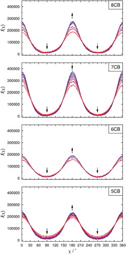
The integrated intensity profiles versus χ obtained from the background-subtracted scattering patterns of the four compounds across a range of temperatures are shown in Figure 4. These profiles illustrate the general change in shape with temperature, with the peaks becoming sharper and more intense on lowering the temperature, along with a decreasing baseline intensity between the peaks. The total integrated intensity increased on lowering the temperature, by ca. 8–14% across the respective temperature ranges used here, which may be attributed to the sharper peaks increasing the total intensity in the integration regions used.

Figure 4. (Colour online) Integrated intensity profiles, I(χ), obtained from the background-subtracted experimental X-ray scattering patterns of 5CB, 6CB, 7CB and 8CB. Curves are coloured according to temperature (listed in the Supporting Information) from the highest (red) to the lowest (blue), and arrows show the direction of change on cooling.

3.1.2. Baseline correction methods

In this work, we have assessed two methods of baseline correction. The first method is to set the minimum value of each integrated intensity profile to zero (zero-offset), and the second is to subtract an experimental estimate of the baseline intensity (baseline-offset). The experimental estimate for the baseline-offset method was obtained by using the scattering image recorded at the lowest temperature for each compound to determine the average value of the intensity in regions close to the wide-angle integration limits and parallel to the director, which are the regions within the integration limits that should have the minimum intensity of scattered radiation. These regions are inevitably somewhat arbitrary, but were defined here as those within 50 pixels of the inner and outer wide-angle integration limits, and within 5° of the director orientation as shown by the shaded regions for 5CB in Figure 5.

Figure 5. Background-subtracted X-ray scattering pattern of 5CB showing the wide-angle integration limits (white rings) and the regions used to estimate the baseline offset (grey-shaded areas). The horizontal white line corresponds to χ = 0°.

3.2. Order parameter determination methods

3.2.1. Leadbetter and Norris method

The first method used in this work is that of Leadbetter and Norris, herein referred to as the LN method. Despite the error in the derivation of Equation (4) used in this approach, as highlighted in the introduction, its widespread use in the liquid crystal literature means it is useful to include it here for comparative purposes. Equation (4) is shown in its expanded form in Equation (7), which is fitted to the experimental data to determine the coefficients, f_2n, which are the coefficients of the orientational distribution function expanded according to Equation (8) [23]. The most widespread method of determining the order parameters, ⟨P₂⟩ and ⟨P₄⟩, from this approach appears to be that of Davidson et al. [23], using Equations (9) and (10) to obtain the values of ⟨cos²β⟩ and ⟨cos⁴β⟩, which may then be used to determine the orientational order parameters, ⟨P₂⟩ = ½(3⟨cos²β⟩ − 1) and ⟨P₄⟩ = ⅛ (35⟨cos⁴β⟩ − 30⟨cos²β⟩ + 3).

(7) $I\left(\chi \right)=f_0+\frac{2}{3}{f}_2{cos}^2\chi +\frac{8}{15}{f}_4{cos}^4\chi +\frac{16}{35}{f}_6{cos}^6\chi +\frac{128}{315}{f}_8{cos}^8\chi +\frac{256}{693}{f}_{10}{cos}^{10}\chi ...$(7)

(8) $f\left(\beta \right)=\sum _{n=0}^{\mathrm{\infty }}{f}_{2n}{cos}^{2n}\beta$(8)

(9) $⟨{cos}^2\beta ⟩=\frac{\sum _{n=0}^{\mathrm{\infty }}\frac{f_{2n}}{2n+3}}{\sum _{n=0}^{\mathrm{\infty }}\frac{f_{2n}}{2n+1}}$(9)

(10) $⟨{cos}^4\beta ⟩=\frac{\sum _{n=0}^{\mathrm{\infty }}\frac{f_{2n}}{2n+5}}{\sum _{n=0}^{\mathrm{\infty }}\frac{f_{2n}}{2n+1}}$(10)

3.2.2. Kratky method

The second method employed is the correct version of the LN method, given by Equation (5), the derivation of which has been described in detail elsewhere [9]. Here, we take an equivalent approach to Davidson et al. which results in the expansion given by Equation (11), which is the correct version of Equation (7) in the LN method, as derived here in the Supporting Information and as recently reported independently [18]. The experimental data are fitted to Equation (11), and values of ⟨P₂⟩ and ⟨P₄⟩ may again be determined via Equations (9) and (10). We refer to this method as the Kratky method.

(11) $I\left(\chi \right)=f_0+\frac{1}{2}{f}_2{cos}^2\chi +\frac{3}{8}{f}_4{cos}^4\chi +\frac{5}{16}{f}_6{cos}^6\chi +\frac{35}{128}{f}_8{cos}^8\chi +\frac{63}{256}{f}_{10}{cos}^{10}\chi ...$(11)

3.2.3. Lovell and Mitchell method

Finally, we also use the method described by Lovell and Mitchell [45], which we refer to as the LM method, given by Equation (6). This method results in the expressions for ⟨P₂⟩ and ⟨P₄⟩ given by Equations (12) and (13), where ⟨P_L⟩_D is the Lth-rank order parameter of the distribution function, and ⟨P_L⟩_I is the Lth-rank order parameter of the experimental integrated intensity profile. Values of ⟨P_L⟩_I are determined from the experimental data via Equation (3), but using discrete summations instead of integrals. In principle, the LM method should yield the same order parameters as those obtained using the Kratky approach because the assumption of a simple equatorial reflection is common to each method. However, the LM method obtains values of ⟨P_L⟩ directly from the experimental intensity profile, whereas the Kratky method relies on fitting the experimental intensity profile to the expansion given in Equation (11) and subsequently determining values of ⟨P_L⟩ from the coefficients of this expansion. Thus, differences between the order parameters obtained from the Kratky and LM methods may arise if an insufficient number of terms in the expansion is used when applying the Kratky method.

(12) $⟨P_2{⟩}_D=-2⟨P_2{⟩}_I$(12)

(13) $⟨P_4{⟩}_D=\frac{8}{3}⟨P_4{⟩}_I$(13)

3.3. Application of the analysis methods to the experimental data

3.3.1. Truncation of expansions in the Kratky and LN methods

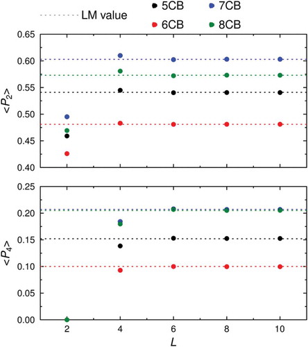
The experimental order parameters of 5CB, 6CB, 7CB and 8CB were initially calculated using the Kratky and LM methods in order to assess the effect of the number of terms used in the expansion applied in Kratky method; the background-subtracted, baseline-offset scattering images obtained at the lowest respective reduced temperatures were used for these analyses. The order parameters, ⟨P₂⟩ and ⟨P₄⟩, determined using the LM method are shown in Figure 6 along with those calculated using the Kratky method, and truncating the expansion in Equation (11) at different values of L. These plots show that the values determined using the LM method are matched closely by those of the Kratky method for values of L ≥ 6, for which differences of ≤0.001 in the values of ⟨P₂⟩ and ⟨P₄⟩ between the methods were found. However, truncating at L = 6 may not necessarily be sufficient for all intensity profiles so all subsequent use of the Kratky method reported here was carried out truncating at L = 10; for consistency, the expansion in the LN method given by Equation (7) was also truncated at L = 10.

Figure 6. (Colour online) Order parameters, ⟨P₂⟩ and ⟨P₄⟩, of 5CB, 6CB, 7CB and 8CB obtained from background-subtracted, baseline-corrected scattering patterns recorded at the lowest respective reduced temperatures using the LM method (dashed lines) and the Kratky method truncating the expansion at different values of L (circles).

3.3.2. Comparison of LN, Kratky, LM and baseline correction methods

The second-rank order parameters, ⟨P₂⟩, of 5CB, 6CB, 7CB and 8CB were determined using the LN, Kratky and LM methods from background-subtracted scattering profiles recorded at a range of temperatures and with either a zero-offset or a baseline-offset, as shown in Figure 7. The values obtained from the Kratky and LM methods were found to differ by ≤0.0001, so these are plotted as a single dataset in Figure 7.

Figure 7. (Colour online) Experimental second-rank order parameters, ⟨P₂⟩, for 5CB, 6CB, 7CB and 8CB, determined from integrated intensity profiles from background-subtracted and either baseline-offset or zero-offset scattering patterns. The vertical dashed line denotes the N-SmA transition of 8CB [57].

For each compound at each temperature, the most significant cause of difference in the ⟨P₂⟩ values arises from whether the intensity profile is zero-offset or baseline-offset, with the difference between the Kratky/LM and LN methods being small in comparison. In each case, the use of a zero-offset causes a significant increase in the order parameter relative to that obtained from a baseline-offset, with differences in ⟨P₂⟩ of up to 0.19. The LN method underestimates the order parameter by 0.014–0.041 from the Kratky/LM methods, generally more so for lower values of ⟨P₂⟩. It is interesting to note that a study of the reliability of order parameters determined from X-ray scattering patterns, carried out using the LN model, concluded that the approach underestimates the true values of ⟨P₂⟩ by ca. 0.03–0.06 [38,39]; the results shown in Figure 7 suggest that this underestimation may at least partially be attributed to the error in Equation (4) in the LN approach.

An equivalent comparison of ⟨P₄⟩ values determined from the same scattering patterns of 5CB, 6CB, 7CB and 8CB was also carried out, as shown in Figure 8. The ⟨P₄⟩ values reveal similar trends to the ⟨P₂⟩ values, but with the baseline-correction having a smaller effect and with smaller differences in magnitude of 0.007–0.014 between the Kratky/LM and LN methods.

Figure 8. (Colour online) Experimental fourth-rank order parameters, ⟨P₄⟩, for 5CB, 6CB, 7CB and 8CB, determined from integrated intensity profiles from background-subtracted and either baseline-offset or zero-offset scattering patterns. The vertical dashed line denotes the N-SmA transition of 8CB [57].

3.3.3. Comparison with reported order parameters

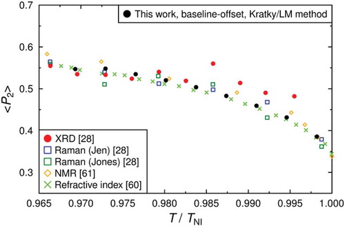
5CB is perhaps the most widely studied mesogenic compound, and as a result there are many reports of its order parameter measured using a variety of techniques. A comparison of ⟨P₂⟩ values determined here using baseline-offset scattering profiles and the Kratky/LM method with those reported from various techniques is shown in Figure 9. The values measured here generally show good agreement with those reported from refractive index [60], Raman [28], and NMR experiments of partially deuterated 5CB [61]. Values from previously reported X-ray studies [28] show good agreement at low reduced temperatures, but appear to overestimate the order parameter at high reduced temperature; this difference is not dissimilar to that shown in Figure S1 in the Supporting Information for zero-offset intensity profiles, which overestimate the order parameters particularly at high reduced temperatures.

Figure 9. (Colour online) Comparison of second-rank order parameters, ⟨P₂⟩, of 5CB obtained from background-subtracted and baseline-offset data using the Kratky/LM method plotted against reduced temperature from this work, and from a range of reported values.

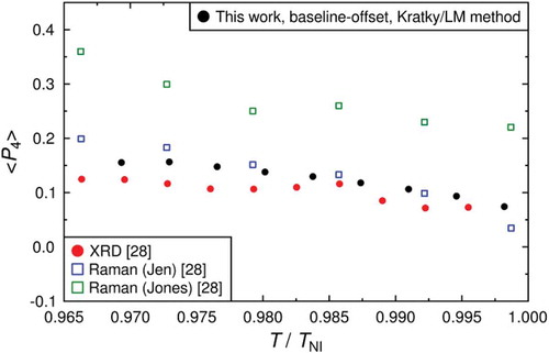
Values of ⟨P₄⟩ are less frequently reported, due to the fewer methods able to determine them in comparison with values of ⟨P₂⟩, but some values have been reported from X-ray and Raman studies, and a comparison with those determined in this study using baseline-offset scattering patterns and the Kratky/LM method are shown in Figure 10. The ⟨P₄⟩ values measured here are in good agreement with those reported from Raman experiments using the Jen method, and are in reasonably good agreement with reported values from X-ray scattering. There is a significant discrepancy with the Raman values determined using the Jones method, but this discrepancy has previously been attributed to nonlinear optical effects in the sample [28].

Figure 10. (Colour online) Comparison of fourth-rank order parameters, ⟨P₄⟩, of 5CB obtained from background-subtracted and baseline-offset data using the Kratky/LM method plotted against reduced temperature from this work, and from a range of reported values.

Using the LN method or, in particular, applying a zero-offset baseline results in a poorer match with reported values than those shown in Figures 9 and 10, as shown in equivalent plots in the Supporting Information (Figures S1–S4). Overall, these comparisons indicate that using X-ray scattering data with appropriate background subtraction and baseline corrections and the Kratky/LM method provide orientational order parameters that are in very good agreement with reported values using different techniques.

In comparison with 5CB, the order parameters of 6CB, 7CB and 8CB are less widely reported in the literature, and we found significant differences between the reported values, which precluded meaningful comparisons with the values we present here. A comparison of the ⟨P₂⟩ and ⟨P₄⟩ order parameters determined here with the values calculated by Maier–Saupe theory [62] is shown for all the compounds in plots in the Supporting Information (Figures S5–S7), and that theoretical model gives a moderate match to the experimental data.

3.3.4. Other possible analysis methods

The methods we have used here to determine the order parameters do not impose any specific form of orientational distribution function within the analysis, and as such they provide a general approach that we consider to be preferable in these studies. Other possible methods include those that assume a particular form of orientational distribution, such as that provided by Maier–Saupe theory, to generate alternative expressions that may be used to fit the experimental data [23]. This general approach may be advantageous in some cases because it can provide a direct test of the match between experiment and the chosen theory.

4. Calculated data generation, analysis and discussion

In order to make an independent assessment of the methods reported in Section 3.3 for the analysis of experimental data, we have used these same methods to analyse calculated X-ray scattering profiles generated from theoretical orientational distributions. This use of calculated data enables differences between the various analysis methods to be assessed for well-defined orientational distributions for which the true order parameters are known.

4.1. Generation of orientational distributions and calculated X-ray scattering data

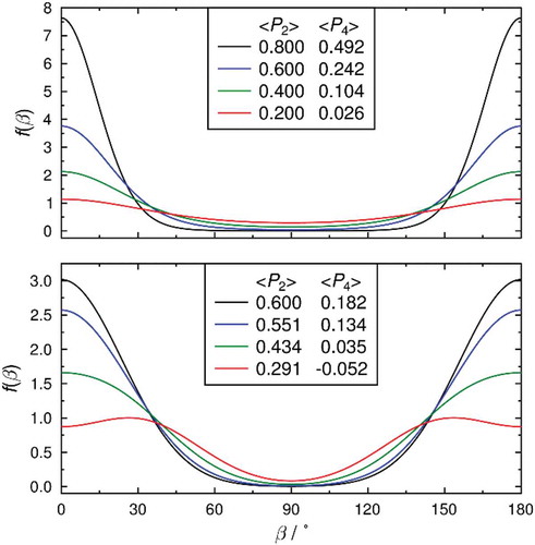
Four maximum entropy orientational distributions were calculated according to Equation (14),[3, 13] with values of the coefficient a chosen to give values of ⟨P₂⟩ = 0.2, 0.4, 0.6 and 0.8, in accordance with Equation (3), to cover the range of values typically measured for liquid-crystalline samples. Four additional orientational distributions that are representative of sugar-loaf and diffuse-cone (volcano) types of distributions were also calculated by first defining f(β) as Gaussian distributions centred at 0° and 180° corresponding to a typical order parameter of ⟨P₂⟩ = 0.6, in accordance with Equation (3), and then splitting each into two identical Gaussian peaks which were sequentially offset by ± 10°, 20° and 30° to give three further distribution functions. The distributions were normalised according to Equation (15), [3] and are shown in Figure 11 along with their associated values of ⟨P₂⟩ and ⟨P₄⟩.

(14) $f\left(\beta \right)={\mathrm{e}}^{a{P}_2\left(cos\beta \right)}$(14)

(15) $\underset{0}{\overset{\pi }{\int }}f\left(\beta \right)sin\beta \mathrm{d}\beta =1$(15)

Figure 11. (Colour online) Maximum entropy orientational distributions (top) and sugar-loaf and diffuse-cone orientational distributions (bottom) with associated order parameters, ⟨P₂⟩ and ⟨P₄⟩.

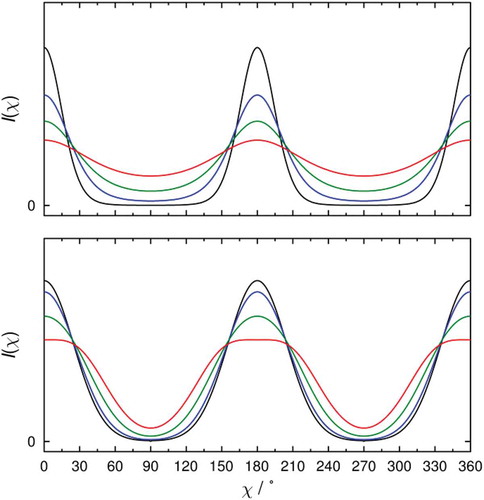
X-ray scattering intensity profiles, I(χ), were then determined by numerical integration of the orientational distributions in Figure 11 in accordance with Equation (5), i.e. using the Kratky method, and these profiles are shown in Figure 12. The calculated intensity profiles determined from the maximum entropy distributions show the peak intensities falling and, crucially, the baseline intensities between the peaks rising with decreasing order parameter, which demonstrates that applying a zero-offset baseline would not be appropriate for the profiles arising from such distributions. A similar pattern is evident from the calculated intensity profiles determined from the sugar-loaf and diffuse-cone distributions, but the peaks broaden and the baselines rise to a lesser extent as the peaks in the orientational distribution become more separated and the order parameters decrease; three further distributions with the Gaussian peaks offset by ± 35°, 40° and 45° resulted in calculated volcano-type profiles for the intensities as well as the distributions at low ⟨P₂⟩ values, and they are shown in the Supporting Information (Figures S8 and S9).

Figure 12. (Colour online) Calculated intensity profiles, I(χ), obtained from the maximum entropy distributions (top) and the sugar-loaf and diffuse-cone distributions (bottom) by numerical integration of Equation (5). The curves are coloured to match the distributions given in Figure 11.

4.2. Application of the analysis methods to the calculated data

4.2.1. Analysis of raw calculated data

The order parameters ⟨P₂⟩ and ⟨P₄⟩ determined from the raw calculated intensity profiles in Figure 12 using the Kratky and LM methods, applied in the same way as described in Section 3.3, were equal to the true order parameters for all of the distributions shown in Figure 11.

Values of ⟨P₂⟩ and ⟨P₄⟩ determined from the raw calculated intensity profiles obtained from the maximum entropy distributions using the LN method are given in Table 1. These values are similar to the true values but, relatively, they underestimate the values increasingly as the distributions broaden, which is generally consistent with the trend in the experimental results at low order parameters shown in Figure 7. Although the relative differences are large in some cases, the absolute differences are all ≤0.045 for these calculated distributions.

Table 1. Values, differences, Δ, and percentage differences, Δ(%), of the true order parameters, ⟨P₂⟩ and ⟨P₄⟩, of the maximum-entropy distributions shown in Figure 11 and those determined using the LN method.

⟨P2⟩				⟨P4⟩
True	LN	Δ	Δ(%)	True	LN	Δ	Δ(%)
0.800	0.796	−0.004	−0.5	0.492	0.488	−0.004	−0.8
0.600	0.572	−0.028	−4.7	0.242	0.228	−0.014	−5.8
0.400	0.355	−0.045	−11.3	0.104	0.090	−0.014	−13.5
0.200	0.163	−0.037	−18.5	0.026	0.021	−0.005	−19.2

Values of ⟨P₂⟩ and ⟨P₄⟩ determined from the raw calculated intensity profiles obtained from the sugar-loaf and diffuse-cone distributions using the LN method are given in Table 2 and, as for the maximum entropy distributions, the LN method underestimates the magnitudes of the order parameters in every case. The values of ⟨P₄⟩ are vital to identifying a diffuse-cone-like distribution experimentally, and negative values of ⟨P₄⟩ have been used to confirm the presence of distributions with probability maxima at β ≠ 0° [14]. Crucially for these distributions, the crossover from positive to negative values of ⟨P₄⟩ occurs at the same point in the data between the different methods, indicating that the error in the LN model is unlikely to invalidate negative ⟨P₄⟩ values determined using this method; the computational results we report here support the conclusion drawn recently from a comparison of experimental data [18].

Table 2. Values, differences, Δ, and percentage differences, Δ(%), of the true order parameters, ⟨P₂⟩ and ⟨P₄⟩, of the diffuse-cone-like distributions shown in Figure 11 and those determined using the LN method.

⟨P2⟩				⟨P4⟩
True	LN	Δ	Δ(%)	True	LN	Δ	Δ(%)
0.600	0.594	−0.006	−1.0	0.182	0.178	−0.004	−2.2
0.551	0.543	−0.008	−1.5	0.134	0.130	−0.004	−3.0
0.434	0.423	−0.011	−2.5	0.035	0.034	−0.001	−2.9
0.291	0.282	−0.009	−3.1	−0.052	−0.042	0.010	19.2

4.2.2. Analysis of zero-offset calculated data

The use of a zero-offset baseline correction was shown to change the experimentally determined order parameters significantly, as discussed above and shown in Figures 7 and 8, and it is therefore useful to assess the impact of zero-offsets for known distributions. The calculated intensity profiles defined and shown in Figure 12 were offset to a zero baseline, and these zero-offset intensity profiles were then used to determine values of ⟨P₂⟩ and ⟨P₄⟩ using the LM method, enabling a comparison of the order parameters before and after a zero-offset was applied.

The order parameters determined from the maximum-entropy distributions are given in Table 3, and show that applying a zero-offset to the baseline has little effect for highly ordered distributions, resulting in only small discrepancies for narrow distributions, but for the broader distributions with lower order parameters the impact is much greater.

Table 3. Values, differences, Δ, and percentage differences of the true order parameters, ⟨P₂⟩ and ⟨P₄⟩, of the maximum-entropy distributions shown in Figure 11 and those determined using the LM method after applying a zero-offset to the calculated scattering intensity profiles.

⟨P2⟩				⟨P4⟩
True	Zero-offset	Δ	Δ(%)	True	Zero-offset	Δ	Δ(%)
0.800	0.806	0.006	0.8	0.492	0.495	0.003	0.6
0.600	0.658	0.058	9.7	0.242	0.266	0.024	9.9
0.400	0.558	0.158	39.5	0.104	0.145	0.041	39.4
0.200	0.476	0.276	138.0	0.026	0.063	0.037	142.3

The order parameters calculated from the zero-offset sugar loaf and diffuse-cone distributions are given in Table 4. The effect of the zero-offset is less significant than for the maximum entropy distributions, but again the discrepancies arising from applying a zero-offset increase with the broader distribution functions. The change of sign in ⟨P₄⟩ calculated using zero-offset intensity profiles occurs at the same point in the data as the change of sign in the true values.

Table 4. Values, differences, Δ, and percentage differences of the true order parameters, ⟨P₂⟩ and ⟨P₄⟩, of the diffuse-cone-like distributions shown in Figure 11 and those determined using the LM method after applying a zero-offset to the calculated scattering intensity profiles.

⟨P2⟩				⟨P4⟩
True	Zero-offset	Δ	Δ(%)	True	Zero-offset	Δ	Δ(%)
0.600	0.606	0.006	1.0	0.182	0.184	0.002	1.1
0.551	0.564	0.013	2.4	0.134	0.138	0.004	3.0
0.434	0.466	0.032	7.4	0.035	0.037	0.002	5.7
0.291	0.350	0.059	20.3	−0.052	−0.062	−0.010	19.2

5. Conclusions

Experimental X-ray scattering data from a series of cyanobiphenyl compounds and calculated X-ray scattering intensity profiles from a set of theoretical orientational distribution functions were used to assess the data processing and analysis methods used to determine the orientational order parameters of uniaxial liquid crystal phases.

For data processing, an appropriate background subtraction was provided readily by using the scattering image from an empty capillary, which is a method that is consistent with that reported generally in the literature. Two baseline correction methods were assessed, using an offset to a minimum either at zero intensity or at a baseline intensity determined experimentally from regions with low scattering intensity, which are two methods that appear to be in general use. The method used for baseline correction was shown to have a significant influence on the values obtained for the order parameters. The use of a zero-offset correction to the computationally generated intensity profiles resulted in the known order parameters being overestimated significantly, particularly for broad distributions with low order parameters where the calculated intensity profiles showed clearly that the minimum will be significantly above zero. The use of experimentally estimated baseline-offset corrections to the experimental scattering profiles of 5CB, 6CB, 7CB and 8CB resulted in order parameters that gave good agreement with reported values that had been determined using a wide range of other experimental techniques, whereas the use of zero-offset corrections gave larger values and a poorer agreement. The difference in order parameter values arising from the choice of baseline correction method was shown to be significantly larger than that arising from the different analysis methods summarised below, and so it would seem beneficial for reports of order parameters determined from X-ray scattering studies of liquid-crystalline materials to detail any baseline correction method that may have been applied. The baseline offset method reported in this work provides a straightforward approach.

For data analysis, the methods of Kratky and Lovell and Mitchell gave essentially identical order parameters from the experimental data by truncating the Kratky expression at L = 6, and the analyses we report were truncated conservatively at L = 10. The popular method within the liquid crystal field proposed by Leadbetter et al. consistently underestimated the magnitude of the values of both ⟨P₂⟩ and ⟨P₄⟩ relative to those obtained using the Kratky/LM methods for all the experimental and computational data analysed in this study, and this discrepancy is attributable to the error in the equations used in the Leadbetter method, as reported elsewhere. Despite the error in the Leadbetter method, the differences arising from this error were relatively small, at ≤0.045 for values of ⟨P₂⟩ and ≤0.014 for values of ⟨P₄⟩ for the computationally generated distributions studied here; moreover, changes from positive to negative values of ⟨P₄⟩ were shown to be consistent between all of the methods. It would appear from our studies that conclusions drawn from reported order parameters determined using the Leadbetter equations should not be discredited, but that detailed quantitative comparisons should be treated with caution, which is consistent with a recent report [18]. It would be preferable for studies of liquid crystals to use the corrected equations rather than the original Leadbetter method, if using this general approach, in order to enable quantitative comparisons to be made between reported studies. However, for the calculation of order parameters alone, the Lovell and Mitchell method would seem to be the most appropriate method due to its simplicity and the direct conversion of order parameters of the intensity profile to order parameters of the orientational distribution function without requiring the truncation of an expansion.

The data processing and analysis methods we have reported and applied here to a series of cyanobiphenyl compounds may be expected to have general applicability to uniaxial liquid crystal phases that give similar, relatively simple scattering patterns. For related systems that give more complex scattering patterns, the general principles outlined here may provide a useful basis for devising slightly modified data processing and analysis methods that are tailored for such systems.

Acknowledgements

We thank Dr Stephen Cowling for experimental assistance and advice. Data from this article are available by request from the University of York Data Catalogue at https://doi.org/10.15124/57d8b69a-c6d8-4a6a-bfae-39814f572860

Disclosure statement

No potential conflict of interest was reported by the authors.

Supplemental material

Supplemental data for this article can be accessed here.

Additional information

Funding

This work was supported by The Engineering and Physical Sciences Research Council (EPSRC) under grant EP/M020584/1 for the development of dyes for liquid crystal applications and the Core Capability grant EP/K039660/1.

References

- Agra-Kooijman DM, Kumar S. Handbook of liquid crystals. 1. Goodby JW, Collings PJ, Kato T, Tschierske C, Gleeson HF, Raynes EP, editors. Weinheim: Wiley; 2014. p. III:10: 11–38.
- Luckhurst GR. Physical properties of liquid crystals: nematics. Dunmur DA, Fukuda A, Luckhurst GR, editors.London: IET;2001. p. 57–88.
- Zannoni C. The molecular dynamics of liquid crystals. Luckhurst GR, Veracini CA, editors. New York: Springer;1994. p. 11–40.
- Luckhurst GR. Biaxial nematic liquid crystals. Luckhurst GR, J. ST, editors. United Kingdom: Wiley;2015.p. 25–54.
- Jen S, Clark NA, Pershan PS, et al. Polarized Raman scattering studies of orientational order in uniaxial liquid crystalline phases. J Chem Phys. 1977;66:4635–4661.
- Arcioni A, Tarroni R, Zannoni C. Can <P4> be obtained from fluorescence depolarization in liquid-crystals. Nuovo Cimento D. 1988;10:1409–1426.
- van Gurp M. The use of rotation matrices in the mathematical description of molecular orientations in polymers. Colloid Polym Sci. 1995;273:607–625.
- Yankova TS, Bobrovsky AY, Vorobiev AK. Order parameters ⟨P2⟩, ⟨P4⟩, and ⟨P6⟩ of aligned nematic liquid-crystalline polymer as determined by numerical simulation of electron paramagnetic resonance spectra. J Phys Chem B. 2012;116:6010–6016.
- Mills TT, Toombes GES, Tristram-Nagle S, et al. Order parameters and areas in fluid-phase oriented lipid membranes using wide angle X-ray scattering. Biophys J. 2008;95:669–681.
- Fan ZX, Buchner S, Haase W, et al. Packing, correlation function, defect structures, and order parameters of liquid‐crystal side‐chain polymers by X‐Ray‐diffraction investigations. J Chem Phys. 1990;92:5099–5106.
- Zhang F, Heiney PA, Srinivasan A, et al. Structure of nematic liquid crystalline elastomers under uniaxial deformation. Phys Rev E. 2006;73:021701.
- Greasty RJ, Richardson RM, Klein S, et al. Electro-induced orientational ordering of anisotropic pigment nanoparticles. Philos Trans A Math Phys Eng Sci. 2013;371:20120257.
- Hamley IW, Garnett S, Luckhurst GR, et al. Orientational ordering in the nematic phase of a thermotropic liquid crystal: a small angle neutron scattering study. J Chem Phys. 1996;104:10046–10054.
- Singh G, Fu J, Agra-Kooijman DM, et al. X-ray and Raman scattering study of orientational order in nematic and heliconical nematic liquid crystals. Phys Rev E. 2016;94:060701.
- Wang Y, Singh G, Agra-Kooijman DM, et al. Room temperature heliconical twist-bend nematic liquid crystal. CrystEngComm. 2015;17:2778–2782.
- Lagerwall ST, Rudquist P, Giesselmann F. The orientational order in so-called de vries materials. Mol Cryst Liq Cryst. 2009;510:148–157.
- Agra-Kooijman DM, Yoon H, Dey S, et al. Origin of weak layer contraction in de Vries smectic liquid crystals. Phys Rev E. 2014;89:032506.
- Agra-Kooijman DM, Fisch MR, Kumar S. The integrals determining orientational order in liquid crystals by X-ray diffraction revisited. Liq Cryst. 2017. doi:10.1080/02678292.2017.1372526.
- Sreenilayam SP, Rodriguez-Lojo D, Panov VP, et al. Design and investigation of de Vries liquid crystals based on 5-phenyl-pyrimidine and (R,R)-2,3-epoxyhexoxy backbone. Phys Rev E. 2017;96:042701.
- Leadbetter AJ, Norris EK. Distribution functions in three liquid crystals from X-ray diffraction measurements. Mol Phys. 1979;38:669–686.
- Leadbetter AJ, Wrighton PG. Order parameters in Sa, Sc and N phases by X-ray diffraction. J Phys-Paris. 1979;C340:234–242.
- Leadbetter AJ. The molecular phyisics of liquid crystals. Luckhurst GR, Gray GW, editors. London: Springer;1979. p. 285–316.
- Davidson P, Petermann D, Levelut AM. The measurement of the nematic order parameter by X-ray scattering reconsidered. J Phys II. 1995;5:113–131.
- Gopalakrishna D, Revannasiddaiah D, Somashekar R. Microscopic order parameter of two nematogenic compounds using X-Rays. Mol Cryst Liq Cryst. 2005;437:121/[1365]-1131/[1375].
- Lagerwall JPF, Giesselmann F, Radcliffe MD. Optical and X-ray evidence of the “de Vries” Sm-A*-Sm-C* transition in a non-layer-shrinkage ferroelectric liquid crystal with very weak interlayer tilt correlation. Phys Rev E. 2002;66:031703.
- Giesselmann F, Germer R, Saipa A. Orientational order in smectic liquid-crystalline phases of amphiphilic diols. J Chem Phys. 2005;123:034906.
- Roberts JC, Kapernaum N, Song Q, et al. Design of liquid crystals with “de Vries-like” properties: frustration between Sma- and Smc-promoting elements. J Am Chem Soc. 2010;132:364–370.
- Sanchez-Castillo A, Osipov MA, Giesselmann F. Orientational order parameters in liquid crystals: a comparative study of X-ray diffraction and polarized Raman spectroscopy results. Phys Rev E. 2010;81:021707.
- Yoon H, Agra-Kooijman DM, Ayub K, et al. Direct observation of diffuse cone behavior in de Vries smectic-a and -c phases of organosiloxane mesogens. Phys Rev Lett. 2011;106:087801.
- Sanchez-Castillo A, Osipov MA, Jagiella S, et al. Orientational order parameters of a de Vries-type ferroelectric liquid crystal obtained by polarized Raman spectroscopy and X-ray diffraction. Phys Rev E. 2012;85:061703.
- Nonnenmacher D, Jagiella S, Song Q, et al. Orientational fluctuations near the smectic a to smectic c phase transition in two “de Vries”-type liquid crystals. ChemPhysChem. 2013;14:2990–2995.
- Mulligan KM, Bogner A, Song Q, et al. Design of liquid crystals with ‘de Vries-like’ properties: the effect of carbosilane nanosegregation in 5-phenyl-1,3,4-thiadiazole mesogens. Journal of Materials Chemistry C. 2014;2:8270–8276.
- Vita F, Hegde M, Portale G, et al. Molecular ordering in the high-temperature nematic phase of an all-aromatic liquid crystal. Soft Matter. 2016;12:2309–2314.
- Kuiper S, Norder B, Jager WF, et al. Elucidation of the orientational order and the phase diagram of p-quinquephenyl. J Phys Chem B. 2011;115:1416–1421.
- Bhattacharjee B, Paul S, Paul R. Order parameter and the orientational distribution function for 4-cyanophenyl-4′-N-heptyl benzoate in the nematic phase. Mol Phys. 1981;44:1391–1398.
- Bates MA, Luckhurst GR. X-ray scattering patterns of model liquid crystals from computer simulation: calculation and analysis. J Chem Phys. 2003;118:6605–6614.
- Savenko SV, Dijkstra M. Accuracy of measuring the nematic order from intensity scatter: a simulation study. Phys Rev E. 2004;70:011705.
- Jenz F, Osipov MA, Jagiella S, et al. Orientational distribution functions and order parameters in “de Vries”-type smectics: a simulation study. J Chem Phys. 2016;145:134901.
- Jenz F, Jagiella S, Glaser MA, et al. Reliability of orientational order parameters determined from two-dimensional X-ray diffraction patterns: a simulation study. ChemPhysChem. 2016;17:1568–1572.
- Burger C, Ruland W. Evaluation of equatorial orientation distributions. J Appl Crystallogr. 2006;39:889–891.
- Kratky O. Zum Deformationsmechanismus Der Faserstoffe, I. Kolloid-Zeitschrift. 1933;64:213–222.
- Mills TT, Tristram-Nagle S, Heberle FA, et al. Liquid-liquid domains in bilayers detected by wide angle X-ray scattering. Biophys J. 2008;95:682–690.
- Tristram-Nagle S, Kim DJ, Akhunzada N, et al. Structure and water permeability of fully hydrated diphytanoylPC. Chem Phys Lipids. 2010;163:630–637.
- Boscia AL, Treece BW, Mohammadyani D, et al. X-ray structure, thermodynamics, elastic properties and MD simulations of cardiolipin/dimyristoylphosphatidylcholine mixed membranes. Chem Phys Lipids. 2014;178:1–10.
- Lovell R, Mitchell GR. Molecular orientation distribution derived from an arbitrary reflection. Acta Crystallogr A. 1981;37:135–137.
- Mitchell GR, Guo W, Davis FJ. Liquid crystal elastomers based upon cellulose derivatives. Polymer. 1992;33:68–74.
- Dreher S, Zachmann HG, Riekel C, et al. Determination of the chain orientation in liquid crystalline polymers by means of microfocus X-ray scattering measurements. Macromolecules. 1995;28:7071–7074.
- Komp A, Finkelmann H. A new type of macroscopically oriented smectic-a liquid crystal elastomer. Macromol Rapid Commun. 2007;28:55–62.
- Kramer D, Finkelmann H. Breakdown of layering in frustrated smectic-a elastomers. Macromol Rapid Commun. 2007;28:2318–2324.
- Sánchez-Ferrer A, Finkelmann H. Uniaxial and shear deformations in smectic-C main-chain liquid-crystalline elastomers. Macromolecules. 2008;41:970–980.
- Krause S, Zander F, Bergmann G, et al. Nematic main-chain elastomers: coupling and orientational behavior. Comptes Rendus Chimie. 2009;12:85–104.
- Storz R, Komp A, Hoffmann A, et al. Phase biaxility in smectic-a side-chain liquid crystalline elastomers. Macromol Rapid Commun. 2009;30:615–621.
- Zander F, Finkelmann H. State of order of the crosslinker in main-chain liquid crystalline elastomers. Macromol Chem Phys. 2010;211:1167–1176.
- Sánchez-Ferrer A, Finkelmann H. Polydomain–monodomain orientational process in smectic-C main-chain liquid-crystalline elastomers. Macromol Rapid Commun. 2011;32:309–315.
- Torras N, Zinoviev KE, Esteve J, et al. Liquid-crystalline elastomer micropillar array for haptic actuation. Journal of Materials Chemistry C. 2013;1:5183–5190.
- Vancso GJ. Orientation factors and orientation distribution function of anisotropic polymer glasses determined by X-ray scattering: a comparison of different evaluation methods. Polym Bull. 1990;24:233–240.
- Hird M. Physical properties of liquid crystals: nematics. Dunmur DA, Fukuda A, Luckhurst GR, editors.London: IET;2001.p. 3–16.
- R Core Team. R: A language and environment for statistical computing. Vienna, Austria: R Foundation for Statistical Computing; 2014.
- Wolfram Research Inc. Mathematica 11.0. Champaign (IL): Wolfram Research, Inc.; 2016.
- Horn RG. Refractive indices and order parameters of two liquid crystals. J Phys France. 1978;39:105–109.
- Emsley JW, Luckhurst GR, Stockley CP. The deuterium and proton-{deuterium} N.M.R. spectra of the partially deuteriated nematic liquid crystal 4-N-pentyl-4′-cyanobiphenyl. Mol Phys. 1981;44:565–580.
- Maier W, Saupe A. Eine einfache molekular-statistische theorie der nematischen kristallinflüssigen phase. Teil II. Z Naturforsch. 1960;15a:287–292.