Rapid thickness mapping of free-standing smectic films using colour information of reflected light

ABSTRACT

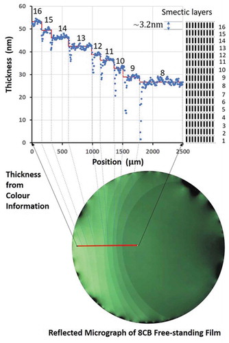
A practical method to rapidly obtain the 2D thickness distribution in free-standing smectic films is developed based on the colour information of reflected image of the film. The red(R), green(G) and blue(B) colour coordinates from each pixel of a colour camera is normalised by the local intensity and is then quantitatively analysed in reference to the theoretical reflection spectra evaluated as a function of the film thickness. Results from the optical system employing a standard stereomicroscope can clearly discriminate a single-layer step over a wide range of thicknesses and provide thickness values with a precision better than 1 nm.

GRAPHICAL ABSTRACT

KEYWORDS:

• Thickness mapping
• free-standing smectic films
• reflected light
• MATLAB
• colour information
• 2D imaging

Introduction

Smectic liquid crystals are a two-dimensional liquid comprised of a stack of monomolecular layers, in each of which molecular positions are more or less translationally disordered [1–3]. The lamellar nature of smectics allows an easy preparation suspended free-standing films, similar to soap films, with the thickness quantised in the unit of the smectic layer [4,5]. The thickness can span a wide range of magnitude from several hundred down to two monolayers, heavily dependent on the preparation conditions.

For the ready availability, the free-standing smectic films have been extensively utilised as a tractable 2D softmatter system for the last several decades. Since the physical and structural properties of free-standing films are critically dependent on the thickness $h$, or equivalently the number of layers $N$, the measurement of film thickness has always been an essential part of any experimental studies of smectic films. The standard technique from the earliest study is to measure the optical reflectivity for a collimated light, relying on the Fresnel formula of multiple reflections that indicates that the reflectivity is proportional to $h^2\propto N^2$ [4–13]. Although this method works well for thin films up to $N\sim 15$, provided that the intensity reference is accurately available, it ceases to be an adequate approach when these conditions are not met as in the case of 2D imaging of static and nonuniform films.

A complementary method, which works for thicker films, is to infer the thickness from the colour or the interferogram. As well experienced for soap films, multiple interference of light through the film leads to a vivid colour depending on the thickness [13,14]. The colour depends on a number of factors, in addition to thickness, including but not limited to the spectrum and the angle of incidence of illumination, and the colour sensitivity of the observer. As long as the colour is visually evaluated, this approach remains to be qualitative, giving only a crude measure of the thickness in spite of the merit that the intensity reference is not required. If the interferogram is measured to make the colour observation more quantitative, it becomes a cumbersome process to make it inadequate for 2D analysis [15–19].

In the spirit of Maxwell’s theory of colour vision [20], the purpose of this paper is to provide a practical method that combines the two existing methods, taking advantage of state-of-the-art imaging and lighting devices, in order to realise a fast and quantitative colour-based technique that allows rapid mapping of the thickness of the free-standing film. We describe below the principle of the method and implementation in detail, followed by the results of applications to free-standing films of a smectic A liquid crystal.

Principle of the method

We aim to link quantitatively the thickness of the free-standing film to the colour of the reflected light in such a way that the image data from a colour camera can be directly exploited for 2D thickness mapping. Let $I\left(\lambda \right)$ be the spectral intensity of the illumination at wavelength $\lambda$ and $R\left(\lambda ,h\right)$ be the reflectivity of the film with the thickness $h$. Then, the reflected light spectrum is given by $I_r\left(\lambda \right)=R\left(\lambda ,h\right)I\left(\lambda \right)$. The colour camera captures the reflected light and decomposes the light intensity into three colour components, i.e., red (R), green (G) and blue (B), for each pixel through colour filters dedicated to R, G and B. The transmission spectra of the colour filters are unique to each camera brand, and we denote them as $f_R\left(\lambda \right)$, $f_G\left(\lambda \right)$ and $f_B\left(\lambda \right)$. For each pixel, the camera provides the colour coordinates as

(1) $X=\int f_R\left(\lambda \right)I_r\left(\lambda \right)d\lambda =\int f_R\left(\lambda \right)R\left(\lambda ,h\right)I\left(\lambda \right)d\lambda ,$(1)

(2) $Y=\int f_G\left(\lambda \right)I_r\left(\lambda \right)d\lambda =\int f_G\left(\lambda \right)R\left(\lambda ,h\right)I\left(\lambda \right)d\lambda ,$(2)

(3) $Z=\int f_B\left(\lambda \right)I_r\left(\lambda \right)d\lambda =\int f_B\left(\lambda \right)R\left(\lambda ,h\right)I\left(\lambda \right)d\lambda .$(3)

To remove the influence of intensity and extract the pure information of colour, we normalise the bare coordinates as

(4) $\left(\bar{X},\bar{Y},\bar{Z}\right)=\frac{1}{\sqrt{X^2+Y^2+Z^2}}\left(X,Y,Z\right)$(4)

With this definition, the normalised colour coordinates are graphically represented as a point on a unit sphere in the $\bar{X},\bar{Y},\bar{Z}$ colour space. Our goal here is to develop a practical scheme, by which the thickness $h$ is accurately evaluated from the 3D colour data $\left(\bar{X},\bar{Y},\bar{Z}\right)$.

The colour of the suspended film in the air originates from the interference of reflection through the top and the bottom surfaces of the film, as illustrated in Figure 1. For simplicity, we first consider the reflection of monochromatic light of wavelength $\lambda$ from an optically isotropic film of thickness $h$. The refractive index of the film, which is, in general, a function of $\lambda$, is written as $n$. For obliquely incident light at the angle of incidence ${\theta }_i$, the Fresnel formulas of reflection at the top surface read

(5) $r_s=\frac{\mathrm{c}\mathrm{o}\mathrm{s}{\theta }_i-n\mathrm{c}\mathrm{o}\mathrm{s}{\theta }_t}{\mathrm{c}\mathrm{o}\mathrm{s}{\theta }_i+n\mathrm{c}\mathrm{o}\mathrm{s}{\theta }_t}$(5)

(6) $r_p=\frac{n\mathrm{c}\mathrm{o}\mathrm{s}{\theta }_i-\mathrm{c}\mathrm{o}\mathrm{s}{\theta }_t}{n\mathrm{c}\mathrm{o}\mathrm{s}{\theta }_i+\mathrm{c}\mathrm{o}\mathrm{s}{\theta }_t}$(6)

Figure 1. Multiple reflection from the free-standing film in air

where ${\theta }_t$ is the angle of refraction connected to ${\theta }_i$ via Snell’s law $\mathrm{s}\mathrm{i}\mathrm{n}{\theta }_i=n\mathrm{s}\mathrm{i}\mathrm{n}{\theta }_t$, and $r_s$ and $r_p$ refer to the coefficients of reflection for s-polarised (polarisation perpendicular to the incidence plane) and p-polarised (polarisation parallel to the plane of incidence) waves, respectively [21]. The coefficients of transmission at the top surface are similarly given, but it suffices here to note the following relations:

(7) $t_{a\to f}^s{t}_{f\to a}^s=1-r_s^2,$(7)

(8) $t_{a\to f}^p{t}_{f\to a}^p=1-r_p^2,$(8)

where the subscript $a\to f$ indicates the transmission from the air to the film and vice versa. The reflection coefficients at the bottom surface for s-polarised and p-polarised waves are given by $-r_s$ and $-r_p$. The extra optical phase added to the light wave upon every reflection is given by

(9) $\beta =\frac{4\pi nh}{\lambda }\mathrm{c}\mathrm{o}\mathrm{s}{\theta }_t$(9)

Summing up the infinite series of reflections with the aid of Eqs. (4)(4) $\left(\bar{X},\bar{Y},\bar{Z}\right)=\frac{1}{\sqrt{X^2+Y^2+Z^2}}\left(X,Y,Z\right)$(4) -(8(8) $t_{a\to f}^p{t}_{f\to a}^p=1-r_p^2,$(8) ), we obtain the total reflection coefficients from the film as follows:

(10) ${\bar{r}}_s=r_s\frac{1-e^{i\beta }}{1-r_s^2{e}^{i\beta }}$(10)

(11) ${\bar{r}}_p=r_p\frac{1-e^{i\beta }}{1-r_p^2{e}^{i\beta }}$(11)

The reflectivity of the film for unpolarised illumination is obtained as

(12) $R\left(\lambda ,h\right)=\frac{1}{2}{\left|{\bar{r}}_s\right|}^2+\frac{1}{2}{\left|{\bar{r}}_p\right|}^2=\frac{1-\mathrm{c}\mathrm{o}\mathrm{s}\beta }{r_s^2+r_s^{-2}-2\mathrm{c}\mathrm{o}\mathrm{s}\beta }+\frac{1-\mathrm{c}\mathrm{o}\mathrm{s}\beta }{r_p^2+r_p^{-2}-2\mathrm{c}\mathrm{o}\mathrm{s}\beta }$(12)

For normal incidence (${\theta }_i={\theta }_t=0$), the s- and p-polarisations are equivalent, i.e. $-r_s=r_p$, and the above equation reduces to the well-known formula of multiple-beam interference. Assuming the angle of incidence is small, we expand the reflection coefficients up to the cubic order of ${\theta }_i$:

(13) $r_s\approx -\frac{n-1}{n+1}\left(1+\frac{1}{n}{\theta }_i^2\right)$(13)

(14) $r_p\approx \frac{n-1}{n+1}\left(1-\frac{1}{n}{\theta }_i^2\right)$(14)

Substituting Eqs.(13)(13) $r_s\approx -\frac{n-1}{n+1}\left(1+\frac{1}{n}{\theta }_i^2\right)$(13) and (14(14) $r_p\approx \frac{n-1}{n+1}\left(1-\frac{1}{n}{\theta }_i^2\right)$(14) ) in Eq.(12(12) $R\left(\lambda ,h\right)=\frac{1}{2}{\left|{\bar{r}}_s\right|}^2+\frac{1}{2}{\left|{\bar{r}}_p\right|}^2=\frac{1-\mathrm{c}\mathrm{o}\mathrm{s}\beta }{r_s^2+r_s^{-2}-2\mathrm{c}\mathrm{o}\mathrm{s}\beta }+\frac{1-\mathrm{c}\mathrm{o}\mathrm{s}\beta }{r_p^2+r_p^{-2}-2\mathrm{c}\mathrm{o}\mathrm{s}\beta }$(12) ), we find that the reflectivity of unpolarised light is not dependent on the angle of incidence up to the cubic order of ${\theta }_i$,

(15) $R\left(\lambda ,h\right)=2\frac{1-\mathrm{c}\mathrm{o}\mathrm{s}\beta }{r_0^2+r_0^{-2}-2\mathrm{c}\mathrm{o}\mathrm{s}\beta }$(15)

where

(16) $r_0=\frac{n-1}{n+1}$(16)

Numerical calculations confirm that the relative error in the approximation[Eq.(15(15) $R\left(\lambda ,h\right)=2\frac{1-\mathrm{c}\mathrm{o}\mathrm{s}\beta }{r_0^2+r_0^{-2}-2\mathrm{c}\mathrm{o}\mathrm{s}\beta }$(15) )] is less than 0.05% at ${\theta }_i={10}^{\circ }$ and less than 0.8% at ${\theta }_i={20}^{\circ }$ for $n=1.5$. Hereafter, we always assume the illumination is unpolarised, and use the approximate reflectivity, Eq.(15)(15) $R\left(\lambda ,h\right)=2\frac{1-\mathrm{c}\mathrm{o}\mathrm{s}\beta }{r_0^2+r_0^{-2}-2\mathrm{c}\mathrm{o}\mathrm{s}\beta }$(15) .

Figure 2 shows the simulated reflection and the corresponding colour as a function of the film thickness up to 600 nm based on Eqs. (1)(1) $X=\int f_R\left(\lambda \right)I_r\left(\lambda \right)d\lambda =\int f_R\left(\lambda \right)R\left(\lambda ,h\right)I\left(\lambda \right)d\lambda ,$(1) -(4(4) $\left(\bar{X},\bar{Y},\bar{Z}\right)=\frac{1}{\sqrt{X^2+Y^2+Z^2}}\left(X,Y,Z\right)$(4) ) and (15(15) $R\left(\lambda ,h\right)=2\frac{1-\mathrm{c}\mathrm{o}\mathrm{s}\beta }{r_0^2+r_0^{-2}-2\mathrm{c}\mathrm{o}\mathrm{s}\beta }$(15) ) for a hypothetical illumination comprised of three monochromatic light sources of unit intensity at ${\lambda }_R=$ 650 nm, ${\lambda }_G=$550 nm and ${\lambda }_B=$450 nm, i.e., $I\left(\lambda \right)=\delta \left(\lambda -{\lambda }_R\right)+\delta \left(\lambda -{\lambda }_G\right)+\delta \left(\lambda -{\lambda }_B\right)$, and a camera with the filter characteristics of $f_R\left({\lambda }_R\right)=f_G\left({\lambda }_G\right)=f_B\left({\lambda }_B\right)=1$ and $f_R\left(\lambda \right)=f_G\left(\lambda \right)=f_B\left(\lambda \right)=0$ otherwise. The refractive index is assumed constant at $n=$1.8 independent of the wavelength. 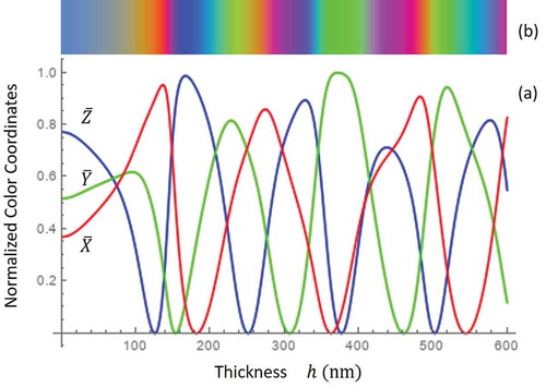The oscillatory behaviour of reflection comes primarily from the factor $1-\mathrm{c}\mathrm{o}\mathrm{s}\beta$, and shows minima at $h=m\lambda /2ncos{\theta }_t$and maxima at $h=\left(m+\frac{1}{2}\right)\lambda /2ncos{\theta }_t$ for nonzero integer $m=0,1,\mathrm{2..}$, where the reflected lights from the top and the bottom surfaces interfere destructively or constructively. The normalised colour coordinates, indicating only the colour information, get more complicated due to the normalisation constraint (Figure 3). One of the most noticeable differences is that as $h\to 0$, the reflection intensities decrease as $h^2$. But the normalised colour coordinates $\left(\bar{X},\bar{Y},\bar{Z}\right)$ converge to a universal point $\left({\lambda }_R^{-2},{\lambda }_G^{-2},{\lambda }_B^{-2}\right)/\sqrt{{\lambda }_R^{-4}+{\lambda }_G^{-4}+{\lambda }_B^{-4}}$, which is solely determined by the illumination spectrum and the transmission functions of colour filters of the camera.

Figure 2. (Colour online) (a) Simulated RGB colour coordinates for the three-colour light source emitting at 650 nm, 550 nm and 450 nm for thickness $h$ from 0–600 nm, and (b) the colour of reflection. The refractive index of the film is $n=$1.8

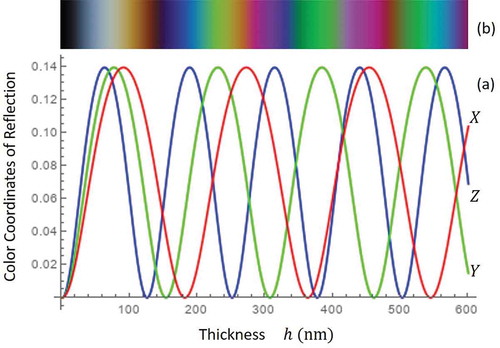
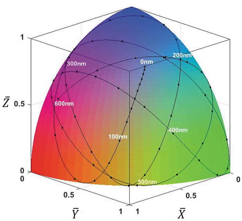
Figure 3. (Colour online) (a) Normalised colour coordinates for simulated reflections for the three-colour light source, and (b) the pure colour of reflection as a function of the thickness

As evident in Figures 2 and 3, although the colour of the reflection provides humans with a clue with which to infer the thickness of the film, the human vision is not capable of telling a minute difference in colour due to few nanometres of thickness change. Let $\left({\bar{X}}_e,{\bar{Y}}_e,{\bar{Z}}_e\right)$ be an experimentally obtained data from the camera. The present method consists in solving the equation

(17) $\left({\bar{X}}_e,{\bar{Y}}_e,{\bar{Z}}_e\right)=\left(\bar{X}\left(h\right),\bar{Y}\left(h\right),\bar{Z}\left(h\right)\right)$(17)

for $h$. Since the colour coordinates are oscillatory as a function of $h$, the equation${\bar{X}}_e=\bar{X}\left(h\right)$, for example, has multiple solutions, $h_X^1,h_X^2,h_X^3\dots$, and so do ${\bar{Y}}_e=\bar{Y}\left(h\right)$ and ${\bar{Z}}_e=\bar{Z}\left(h\right).$ The correct solution should be the one that satisfies

(18) $h_X^i=h_Y^j=h_Z^k$(18)

for appropriate $i,j,$ and $k$ from the pool of possible solutions.

An intuitively straightforward and programmatically more convenient way to identify the solution is to plot the normalised colour coordinates on a unit sphere, as shown in Figure 4, which will be hereafter referred to as the colour quadrant. The simulated normalised colour coordinates $\left(\bar{X}\left(h\right),\bar{Y}\left(h\right),\bar{Z}\left(h\right)\right)$ form a trajectory inside the positive quadrant of the unit sphere. Points on the trajectory give the colour of the film at the thickness. We can observe that the trajectory intercepts itself at a limited number of points, which then guarantees that the solution, Eq.(18(18) $h_X^i=h_Y^j=h_Z^k$(18) ), is unique except for the intersections. Provided the illumination spectrum, the colour filter functions of the camera and the refractive index are precisely known, the observed $\left({\bar{X}}_e,{\bar{Y}}_e,{\bar{Z}}_e\right)$ should fall on the simulated trajectory, and the $h$-value at the landing point gives the thickness of the film.

Figure 4. (Colour online) Normalised colour coordinates plotted on the unit sphere colour space (colour quadrant). The solid line shows the trajectory of $\left(\bar{X}\left(h\right),\bar{Y}\left(h\right),\bar{Z}\left(h\right)\right)$ for $h=$0 – 600 nm. Neighbouring dots are separated by 10 nm

Since the illumination consists of three monochromatic sources in red, green and blue bands in this simulation, the trajectory can reach the edge of the colour space where at least either of $\bar{X}$, $\bar{Y}$ or $\bar{Z}$ vanishes. The dots on the trajectory are plotted for every 10 nm of thickness change. Below 100 nm, the accompanying change of the colour coordinates decreases approximately proportional to $h$, making it increasingly difficult to determine the thickness accurately. The impact of errors in $\left({\bar{X}}_e,{\bar{Y}}_e,{\bar{Z}}_e\right)$ upon the accuracy of the thickness, the determination can be assessed by expanding Eq.(4)(4) $\left(\bar{X},\bar{Y},\bar{Z}\right)=\frac{1}{\sqrt{X^2+Y^2+Z^2}}\left(X,Y,Z\right)$(4) up to first order in $\delta h$.

Note the identity

(19) $\delta \bar{X}=\bar{X}\left\{{\bar{Y}}^2\left(\frac{\delta X}{X}-\frac{\delta Y}{Y}\right)+{\bar{Z}}^2\left(\frac{\delta X}{X}-\frac{\delta Z}{Z}\right)\right\}$(19)

and similar equations for $\delta \bar{Y}$ and $\delta \bar{Z}$, and that

(20) $\delta R\left(\lambda ,h\right)=\frac{8\pi n\mathrm{c}\mathrm{o}\mathrm{s}{\theta }_t}{\lambda }\frac{{\left(r_0-r_0^{-1}\right)}^2\mathrm{s}\mathrm{i}\mathrm{n}\beta }{{\left(r_0^2+r_0^{-2}-2\mathrm{c}\mathrm{o}\mathrm{s}\beta \right)}^2}\delta h$(20)

holds to first order in $\delta h$. For the three-colour illumination as used above, $\delta X/X=\delta R\left({\lambda }_R,h\right)/R\left({\lambda }_R,h\right)$, etc. The arc length $\delta s$ on the trajectory corresponding to the change of thickness by $\delta h$ can be evaluated as

(21) $\delta s=\sqrt{\delta {\bar{X}}^2+\delta {\bar{Y}}^2+\delta {\bar{Z}}^2}$(21)

in combination with Eqs. (19)(19) $\delta \bar{X}=\bar{X}\left\{{\bar{Y}}^2\left(\frac{\delta X}{X}-\frac{\delta Y}{Y}\right)+{\bar{Z}}^2\left(\frac{\delta X}{X}-\frac{\delta Z}{Z}\right)\right\}$(19) and (20(20) $\delta R\left(\lambda ,h\right)=\frac{8\pi n\mathrm{c}\mathrm{o}\mathrm{s}{\theta }_t}{\lambda }\frac{{\left(r_0-r_0^{-1}\right)}^2\mathrm{s}\mathrm{i}\mathrm{n}\beta }{{\left(r_0^2+r_0^{-2}-2\mathrm{c}\mathrm{o}\mathrm{s}\beta \right)}^2}\delta h$(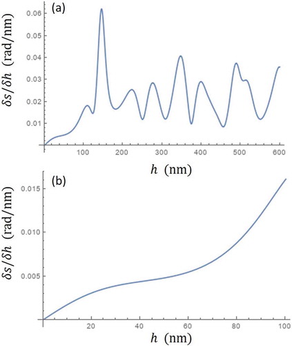20) ). Shown in Figure 5 is the arc length, thus calculated per 1 nm of thickness change as a function of thickness. For film thicknesses larger than 100 nm, it is seen that $\delta s/\delta h>0.01$rad/nm, implying that with a relative intensity resolution of 1% (by the camera), an accuracy of thickness measurement better than 1 nm is possible. For thinner films less than 100 nm; however, the sensitivity of reflection colour to thickness variation steadily declines to 0 at $h=$0 nm. In particular, to measure thickness reliably below 10 nm, it is required to achieve a 0.1% intensity resolution. A regular 8-bit colour camera cannot serve the purpose. Given the inherent low reflection from thinnest films, it sets a demanding requirement on the performance of the camera in terms of sensitivity and intensity resolution. Furthermore, lighting and imaging conditions must be tactically selected to make full use of the dynamic range of the camera.

Figure 5. (Colour online) Arc length $\delta s$ per 1 nm of thickness change for the three-colour light source. (a) $h=$0 – 600 nm. (b) Magnified view of (a) for $h=$0 – 100 nm

We finally consider the effect of dispersion in the refractive index. To be specific, let us employ Cauchy’s dispersion equation:

(22) $n=A+\frac{B}{{\lambda }^2}$(22)

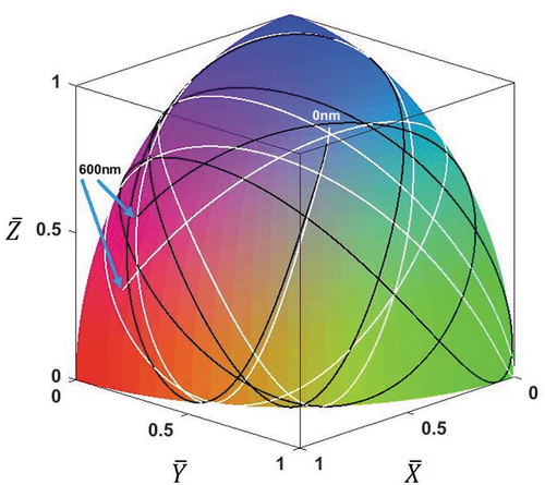
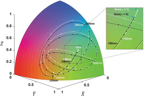
where $A$ and $B$ are constants. The refractive index at $\lambda =$550 nm is fixed at $n=$1.8 to make a comparison with the previous results. And we assume $B=2\times {10}^4$nm² so that $n\left(450\mathrm{n}\mathrm{m}\right)=$1.833 and $n\left(650\mathrm{n}\mathrm{m}\right)=1.781$. As depicted in Figure 6, the point of zero thickness shifts according to the variations of the refractive index at the wavelengths of the light sources. Its effect on the overall shape of the trajectory is more significant as the thickness increases due to the increasing optical phase differences through the film. Since the dispersion of the refractive index is known only for a limited number of representative liquid crystals, it becomes in practice necessary to start with a constant refractive index and adjust the dispersion parameters to best fit the experimental data to the trajectory.

Figure 6. (Colour online) Colour-thickness trajectory on the colour quadrant for the dispersive refractive index (White line). Black line is the trajectory for a constant refractive index

In the limit of zero thickness $h\to 0$, the reflectivity Eq.(15)(15) $R\left(\lambda ,h\right)=2\frac{1-\mathrm{c}\mathrm{o}\mathrm{s}\beta }{r_0^2+r_0^{-2}-2\mathrm{c}\mathrm{o}\mathrm{s}\beta }$(15) is approximated as

(23) $R\left(\lambda ,h\right)\approx \frac{{\pi }^2}{{\lambda }^2}{h}^2{\left(n^2-1\right)}^2\mathrm{c}\mathrm{o}{\mathrm{s}}^2{\theta }_t$(23)

which is valid for $h\ll \lambda /8n\mathrm{c}\mathrm{o}\mathrm{s}{\theta }_t$. It generally follows from the definition of the normalised colour coordinates that if the refractive index is not dependent on the wavelength, i.e. $B=0$, the limiting colour of reflection for vanishing film thickness is uniquely fixed only by the illumination spectrum and the filter transmission functions regardless of the value of the refractive index. Since the factor, ${\left(n^2-1\right)}^2\mathrm{c}\mathrm{o}{\mathrm{s}}^2{\theta }_t$, is an increasing function of $n$, a positive increase in $B$ results in an increase in the blue normalised coordinate $\bar{Z}$ and a decrease in the red normalised coordinate $\bar{X}$ according to Eq.(19)(19) $\delta \bar{X}=\bar{X}\left\{{\bar{Y}}^2\left(\frac{\delta X}{X}-\frac{\delta Y}{Y}\right)+{\bar{Z}}^2\left(\frac{\delta X}{X}-\frac{\delta Z}{Z}\right)\right\}$(19) as shown in Figure 6.

The inability of the present method to absolutely fix the colour coordinates for zero thickness, independent from the instrumental and material parameters, is the most serious weakness of the present method when compared to the standard technique relying on the intensity. Since the refractive index of the film, the illumination spectrum and the transmission functions of colour filter are among others all subject to certain degrees of experimental errors, the origin of the colour trajectory at zero thickness suffers a concomitant unpredictable uncertainty, making it increasingly less reliable to determine the film thickness towards zero. To alleviate this difficulty, we make use of Eq.(23)(23) $R\left(\lambda ,h\right)\approx \frac{{\pi }^2}{{\lambda }^2}{h}^2{\left(n^2-1\right)}^2\mathrm{c}\mathrm{o}{\mathrm{s}}^2{\theta }_t$(23) and note that the reflectivity of the film $R_F$ is proportional to $h^2$ and that the variations of colour coordinates from the origin must be proportional to the thickness such that $\bar{X}\left(h\right)-\bar{X}\left(0\right)\propto h$. Hence we must have

(24) $\bar{X}\left(h\right)-\bar{X}\left(0\right)\propto h\propto \sqrt{R_F}$(24)

and similar relations for $\bar{Y}$ and $\bar{Z}$. In order to incorporate the influence of the aforementioned systematic errors, a posteriori, an adjustable parameter $\alpha$ is introduced in the original definition of the colour coordinates Eqs.(1)(1) $X=\int f_R\left(\lambda \right)I_r\left(\lambda \right)d\lambda =\int f_R\left(\lambda \right)R\left(\lambda ,h\right)I\left(\lambda \right)d\lambda ,$(1) -(3(3) $Z=\int f_B\left(\lambda \right)I_r\left(\lambda \right)d\lambda =\int f_B\left(\lambda \right)R\left(\lambda ,h\right)I\left(\lambda \right)d\lambda .$(3) ) in the following form:

(25) $X=\underset{{\lambda }_S}{\overset{{\lambda }_L}{\int }}\left(1+\alpha \frac{{\lambda }_S^2}{{\lambda }^2}\right)f_R\left(\lambda \right)R\left(\lambda ,h\right)I\left(\lambda \right)d\lambda$(25)

(26) $Y=\underset{{\lambda }_S}{\overset{{\lambda }_L}{\int }}\left(1+\alpha \frac{{\lambda }_S^2}{{\lambda }^2}\right)f_G\left(\lambda \right)R\left(\lambda ,h\right)I\left(\lambda \right)d\lambda$(26)

(27) $Z=\underset{{\lambda }_S}{\overset{{\lambda }_L}{\int }}\left(1+\alpha \frac{{\lambda }_S^2}{{\lambda }^2}\right)f_B\left(\lambda \right)R\left(\lambda ,h\right)I\left(\lambda \right)d\lambda$(27)

Here ${\lambda }_S$ and ${\lambda }_L$ stand for the wavelengths at the short and long edges of the illumination spectrum. This form is adopted after Cauchy’s dispersion equation, and is expected to cover a variety of wavelength-dependent passive optical effects. For a given optical setup and a liquid crystal under study, the parameter $\alpha$ is determined to best achieve the linear relation in Eq.(24)(24) $\bar{X}\left(h\right)-\bar{X}\left(0\right)\propto h\propto \sqrt{R_F}$(24) for observed results. The impact of $\alpha$ on the position of the zero thickness colour coordinates is readily evaluated by applying Eq.(19)(19) $\delta \bar{X}=\bar{X}\left\{{\bar{Y}}^2\left(\frac{\delta X}{X}-\frac{\delta Y}{Y}\right)+{\bar{Z}}^2\left(\frac{\delta X}{X}-\frac{\delta Z}{Z}\right)\right\}$(19) to Eqs.(25)(25) $X=\underset{{\lambda }_S}{\overset{{\lambda }_L}{\int }}\left(1+\alpha \frac{{\lambda }_S^2}{{\lambda }^2}\right)f_R\left(\lambda \right)R\left(\lambda ,h\right)I\left(\lambda \right)d\lambda$(25) -(27(27) $Z=\underset{{\lambda }_S}{\overset{{\lambda }_L}{\int }}\left(1+\alpha \frac{{\lambda }_S^2}{{\lambda }^2}\right)f_B\left(\lambda \right)R\left(\lambda ,h\right)I\left(\lambda \right)d\lambda$(27) ) as

and similar equations for $\bar{Y}\left(0\right)$ and $\bar{Z}\left(0\right)$. Here, ${{\lambda }^2}_R$, ${{\lambda }^2}_G$ and ${{\lambda }^2}_B$ are weighted averages defined by

(29) $\frac{1}{{{\lambda }^2}_R}=\frac{{\int }_{{\lambda }_S}^{{\lambda }_L}\frac{1}{{\lambda }^2}\frac{{\left(n^2-1\right)}^2}{{\lambda }^2}\mathrm{c}\mathrm{o}{\mathrm{s}}^2{\theta }_t{f}_R\left(\lambda \right)I\left(\lambda \right)d\lambda }{{\int }_{{\lambda }_S}^{{\lambda }_L}\frac{{\left(n^2-1\right)}^2}{{\lambda }^2}\mathrm{c}\mathrm{o}{\mathrm{s}}^2{\theta }_t{f}_R\left(\lambda \right)I\left(\lambda \right)d\lambda }$(29)

which satisfy ${\lambda }_L^2>{{\lambda }^2}_R>{{\lambda }^2}_G>{{\lambda }^2}_B>{\lambda }_S^2$. When $\alpha >0$, $\delta \bar{X}\left(0\right)<0$ and $\delta \bar{Z}\left(0\right)$>0, shifting the zero thickness point towards the north pole. The parameter $\alpha$ allows a fine tuning of the colour-thickness trajectory.

A brief comment is finally in order about the light source. We have used the hypothetical three-colour monochromatic light source that allows an analytical treatment of the measurement scheme. In practice, as is the case in our experiment to be described below, it is more likely that the light source is of more or less broadband. Unlike the monochromatic case, the R, G, B-components of reflection cannot disappear entirely at any finite film thickness. In consequence, the trajectory on the colour quadrant does not touch the edge of the colour quadrant, but shrinks towards inside it. Tighter trajectories are less favourable for accurate estimation of the thickness. The colour filter functions of the camera also have the same effect on the shape of the trajectory; the more sharply peaked the transmission spectra, the larger area the trajectory occupies. Prudent consideration of these factors is required in the implementation of the scheme.

Implementation

Figure 7 shows the optical setup we developed based on the platform of a commercial stereomicroscope with zoom capability (Olympus SZH10, Magnification:0.7X – 7.0X), which employs the common main objective design. The advantage of a stereomicroscope in the present context is that it has dual optical trains, which are symmetrically arranged about the normal axis of the sample. One of the two optical trains that is not connected to the camera port is used for illumination; the light from the fibre bundle is collimated by the eyepiece, which automatically guarantees the Kӧhler illumination on the film, i.e. a collimated illumination. For the symmetry, the other optical train captures the reflection. For the present stereomicroscope, the angle of incidence is fixed at ${\theta }_i={8.9}^{\circ }$, which is sufficiently small to assume the quasi-normality of incidence as described in the previous section for unpolarised illumination (Eq.(15)(15) $R\left(\lambda ,h\right)=2\frac{1-\mathrm{c}\mathrm{o}\mathrm{s}\beta }{r_0^2+r_0^{-2}-2\mathrm{c}\mathrm{o}\mathrm{s}\beta }$(15) ). By physically separating the optical trains, it becomes possible to effectively eliminate optical noises due to reflections from the surfaces of optical components. Also advantageous is that the zoom optics on the illumination path automatically adjusts the beam size of illumination on the film in such a way that the total incident energy remains approximately constant, so the brightness of the image stays roughly the same regardless of magnification.

Figure 7. (Colour online) The optical setup for the thickness measurement system based on a stereomicroscope. The free-standing film is inside a closed chamber with two tilted glass windows

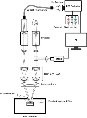
Free-standing films are prepared in a closed chamber. The film is observed through two glass windows that are slightly slanted from the optical path to deflect unnecessary reflections. The light beam reflected from the free-standing film is captured by a CMOS camera (Basler acA1920-155uc, Resolution:1936 x 1216), which can be directly interfaced through USB 3.0 with MATLAB(MathWorks) software running on a Windows 10 computer (XPS 8930, Dell). The camera provides 12bit R,G,B colour coordinate data set for each pixel. For illumination, we used a palm-top LED projector (Optoma Technology ML750) as a digitally controlled light source. The original projection lens was physically inverted to focus the light from the digital micromirror device (DMD) on the entrance aperture of a 5 mm-diameter fibre bundle. The three internal LEDs emitting at around 470 nm, 530 nm and 630 nm are modified to be continuously driven by an external driver in the current control mode. The emission spectra of LEDs are known to slightly shift as the intensity is varied. Hence, to avoid the intensity-dependent spectral change, the DMD works here as a digitally controlled spatial filter. Shown in Figure 8 are the images of illumination as reflected from a plain silver mirror (PF07-03-P01, Thorlabs) placed at the sample plane inside the film chamber at the lowest (0.7X) and the highest (7.0X) magnifications. Due to the limited aperture of the optic train combined with the finite width of fibre bundle, the intensity is peaked at the centre of the field of view and decays towards the edge. At 7.0X magnification, there also exist short scale variations of intensity due probably to imperfections of optics such as dust and surface contaminations. The former intensity variation is systematic, but the latter is unpredictable and is hard to take into proper account in practice. As shown in Figure 8, the $\left(\bar{X},\bar{Y},\bar{Z}\right)$ colour map, normalised via Eq.(4(4) $\left(\bar{X},\bar{Y},\bar{Z}\right)=\frac{1}{\sqrt{X^2+Y^2+Z^2}}\left(X,Y,Z\right)$(4) ), is clearly insensitive to intensity variations of either type except for the edge of the image where the intensity is less than 20% of the peak.

Figure 8. (Colour online) Reference images, cross sectional intensity profiles and colour maps at 0.7X magnification [(a), (b) & (c)] and at 7.0X [(d), (e) & (f)]. A plain silver mirror was set in place of the film. The intensity profiles in (b) & (e) correspond to the cross section in (a) & (b) indicated by broken white lines running the centre

In order to construct the thickness-dependent colour model on the basis of Eqs.(1)(1) $X=\int f_R\left(\lambda \right)I_r\left(\lambda \right)d\lambda =\int f_R\left(\lambda \right)R\left(\lambda ,h\right)I\left(\lambda \right)d\lambda ,$(1) -(3(3) $Z=\int f_B\left(\lambda \right)I_r\left(\lambda \right)d\lambda =\int f_B\left(\lambda \right)R\left(\lambda ,h\right)I\left(\lambda \right)d\lambda .$(3) ) or Eqs.(25)(25) $X=\underset{{\lambda }_S}{\overset{{\lambda }_L}{\int }}\left(1+\alpha \frac{{\lambda }_S^2}{{\lambda }^2}\right)f_R\left(\lambda \right)R\left(\lambda ,h\right)I\left(\lambda \right)d\lambda$(25) -(27(27) $Z=\underset{{\lambda }_S}{\overset{{\lambda }_L}{\int }}\left(1+\alpha \frac{{\lambda }_S^2}{{\lambda }^2}\right)f_B\left(\lambda \right)R\left(\lambda ,h\right)I\left(\lambda \right)d\lambda$(27) ), it is required to characterise the illumination spectrum $I\left(\lambda \right)$ and the transmission functions of colour filters of the camera $f_R\left(\lambda \right)$, $f_G\left(\lambda \right)$ and $f_B\left(\lambda \right)$. In practice, however, it is not so straightforward to measure these functions with a satisfactory level of absolute accuracy as it may first seem. This is because any spectral photodetector has its own wavelength dependence, which cannot be eliminated even after careful calibration to international standards; an accuracy better than 10% is normally considered acceptable [22]. To alleviate this difficulty, we note here that $I\left(\lambda \right)$ and the filter functions appear as a product in the equations, so that it is possible without affecting the left-hand-sides to include an arbitrary function of wavelength $D\left(\lambda \right)$ in such a manner that $I\left(\lambda \right)\to I\left(\lambda \right)D\left(\lambda \right)$ and $f_R\left(\lambda \right)\to f_R\left(\lambda \right)/D\left(\lambda \right)$. Here, $D\left(\lambda \right)$ can be understood as the spectral response of the detector in the former relation, and the latter implies that the identical detector should be used to characterise the filter transmission spectra. As long as the detector can be considered linear, the wavelength dependence of the detector does not affect $\left(\bar{X},\bar{Y},\bar{Z}\right)$.

We used a fibre spectrometer (LR1, ASEQ Instruments) with an optical fibre probe (numerical aperture NA = 0.22) for this purpose. In order to obtain the illumination spectrum $I\left(\lambda \right)$, which should include the effect of microscope optics, a silver mirror (PF07-03-P01, Thorlabs) was placed at the film position as in Figure 8 and measured the spectrum at the exit of the camera port (denoted here as $I_e\left(\lambda \right)$). As shown in Figure 9, Using the reflectance spectrum $R_m\left(\lambda \right)$ of the silver mirror provided by the manufacturer, we obtain the illumination spectrum as $I\left(\lambda \right)=I_e\left(\lambda \right)/R_m\left(\lambda \right)$, which corresponds to the light spectrum at the camera port for a hypothetical perfect mirror placed at the film plane. Finally, we measured the colour filter transmission functions of the CMOS camera as shown in Figure 10. The CMOS camera and the fibre spectrometer were connected to the mutually orthogonal side ports of an integrating sphere (IS236A-4, Thorlabs). Light from a tungsten halogen lamp was fed to a 10 cm diffraction monochromator (CT-10, JASCO) using a light guide, and the monochromated light from the exit slit was directly led to the inlet of the integrating sphere. The monochromator was scanned from 400 nm to 700 nm by 5 nm step. At each step, the image was captured by the CMOS camera along with the spectrum; to obtain the filter transmission function for Red, for example, the total intensity $T_R\left(\lambda \right)$ was obtained by summing up the R-coordinate over all pixels of the image, and the intensity of light $E\left(\lambda \right)$ was obtained from the spectrum. The filter transmission functions are given by

(30) $f_R\left(\lambda \right)=\pi N{A}^2\frac{T_R\left(\lambda \right)}{E\left(\lambda \right)},f_G\left(\lambda \right)=\pi N{A}^2\frac{T_G\left(\lambda \right)}{E\left(\lambda \right)},f_B\left(\lambda \right)=\pi N{A}^2\frac{T_B\left(\lambda \right)}{E\left(\lambda \right)}$(30)

Figure 9. (Colour online) The illumination spectrum $I\left(\lambda \right)$ at the camera port, corrected for a hypothetical perfect mirror reflection (Red line). The black line shows the spectrum observed immediately from the LED projector. The difference is ascribed to loss due to the microscope optics

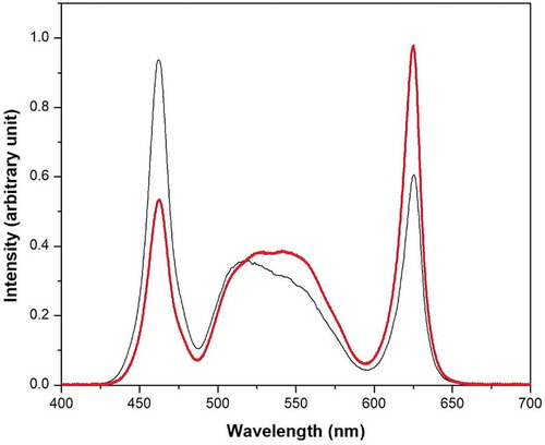
Figure 10. (Colour online) (a) Optical setup for measuring the colour filter transmission functions of the CMOS camera. (b) Transmission functions for Red, Blue and Green colour filters of the camera

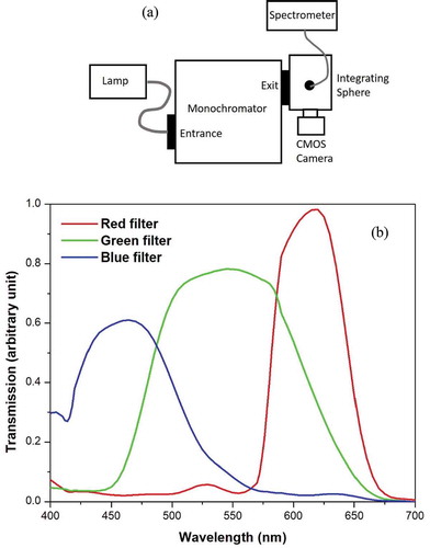
where $\pi N{A}^2$ accounts for the acceptance solid angle of the fibre probe. In Figure 10, the numerical aperture (NA) is assumed constant in the range of illumination spectrum. Note that the filter transmission functions are not absolute, but relative to the spectral sensitivity of the fibre spectrometer we used.

Using the illumination spectrum and the transmission functions of colour filters in Eqs.(1)(1) $X=\int f_R\left(\lambda \right)I_r\left(\lambda \right)d\lambda =\int f_R\left(\lambda \right)R\left(\lambda ,h\right)I\left(\lambda \right)d\lambda ,$(1) -(4(4) $\left(\bar{X},\bar{Y},\bar{Z}\right)=\frac{1}{\sqrt{X^2+Y^2+Z^2}}\left(X,Y,Z\right)$(4) ) and Eqs.(25)(25) $X=\underset{{\lambda }_S}{\overset{{\lambda }_L}{\int }}\left(1+\alpha \frac{{\lambda }_S^2}{{\lambda }^2}\right)f_R\left(\lambda \right)R\left(\lambda ,h\right)I\left(\lambda \right)d\lambda$(25) -(27(27) $Z=\underset{{\lambda }_S}{\overset{{\lambda }_L}{\int }}\left(1+\alpha \frac{{\lambda }_S^2}{{\lambda }^2}\right)f_B\left(\lambda \right)R\left(\lambda ,h\right)I\left(\lambda \right)d\lambda$(27) ), we obtain the colour-thickness trajectory of reflection from free-standing films as shown in Figure 11. Here we assumed the smectic A phase of 4-octyl-4ʹ-cyanobiphenyl (8CB), for which the ordinary refractive index is known to follow Cauchy’s dispersion equation, Eq.(22(22) $n=A+\frac{B}{{\lambda }^2}$(22) ), with

(31) $A=1.4885,B=1.0111\times {10}^4\mathrm{n}{\mathrm{m}}^2$(31)

Figure 11. (Colour online) Colour-thickness trajectory on the colour quadrant for observation of free-standing films of 4-octyl-4ʹ-cyanobiphenyl (8CB) in the present optical setup. The black line and dots indicate the trajectory without adjustment($\alpha =0$). The white line and dots are for the case with $\alpha =1.0$. Dots are plotted every 10 nm

at 21°C [23]. Due to the finite band width of illumination, the trajectory no longer touches the edge of the colour quadrant. In particular, the relatively broad green-light band pushes the trajectory away from the Red-Blue edge. With a finite adjustable parameter $\alpha =1.0$, the trejctory indicated by white line is slightly modified especially near the zero thickness point. For thick film region beyond 150 nm, however, the difference becomes much less significant below 1 nm in thickness. The role of the parameter $\alpha$ is to account for aggregated unknown errors in the refractive index of the film, the illumination spectrum and the transmission functions of colour filters, whose impact is most serious near the zero thickness. Once determined, the value of $\alpha$ should remain the same as long as the film material is not changed.

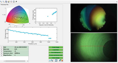
In order to complete the implementation, we developed a MATLAB code that directly grabs image data from the CMOS camera through USB 3.0 interface, plots the colour coordinates for all pixels on the $\bar{X},\bar{Y},\bar{Z}$ colour space and yields the thickness values in reference to the prefabricated colour-thickness trajectory in Figure 11. The code for the thickness evaluation is fully vectorised and can process a large number of data points efficiently. The software offers a neat graphical user interface (GUI) as shown in Figure 12, on which all commands including not limited to ‘Grab Image’ and ‘Cross Sectional Thickness Profile’ can be executed by one click. Although the data points do not necessarily fall exactly on the colour trajectory due to pixel-by-pixel colour shifts of the camera or the slight variation of illumination spectrum, it is straightforward to identify the most plausible thickness for each pixel from the projection of the data point on the colour-thickness trajectory (the closest point on the trajectory).

Figure 12. (Colour online) Graphical User Interface (GUI) of the MATLAB software for thickness mapping of free-standing films. Top right is the real time image of the film, and the bottom right displays the saved image to be analysed. The corresponding colour map on the colour quadrant is shown on the left side with the thickness versus the square root intensity plot (to the right) and the cross sectional thickness profile (centre left) along the red line drawn manually on the target image on the bottom right

Results and discussions

We used a room temperature smectic A liquid crystal, 4-octyl-4ʹ-cyanobiphenyl (8CB), and prepared free-standing films inside the air tight film chamber at 21${ }^{\circ }C$. It is first necessary to determine the adjustable parameter $\alpha$ from observations in the thin film region below 100 nm, where the linear relation Eq.(24)(24) $\bar{X}\left(h\right)-\bar{X}\left(0\right)\propto h\propto \sqrt{R_F}$(24) holds. Figure 13 shows the image of an 8CB free-standing film captured at the lowest magnification, and the plot of colour coordinates along the cross sectional line. The film thickness corresponding to each pixel is obtained from the point of projection of its colour coordinates onto the trajectory. The $\alpha$ value is determined in such a way that the thicknesses thus obtained best satisfy the linearity relation Eq.(24)(24) $\bar{X}\left(h\right)-\bar{X}\left(0\right)\propto h\propto \sqrt{R_F}$(24) with the pixel-wise reflectivity of the film as shown in Figure 14. The reflectivity $R_F$ is obtained as the pixel-wise ratio of the intensity of reflected light from the film divided by the intensity of reflection from the mirror at the same magnification (see Figure 8). This plot not only provides the optimum $\alpha$ value, but also reveals salient features of the present method. The data points are clearly segregated into clusters corresponding to the layered structure of the film. The extension of the cluster in the vertical direction grows as the film thickness decreases, indicating a larger range of error in the thickness. This is consistent with the linearly decreasing thickness-sensitivity as $h\to 0$ shown in Figure 5. It is also of interest to note that the lateral extension, on the other hand, increases as the film becomes thicker, resulting in a larger error in reflectivity. The thickness of the thinnest layer is approximately 20.2$\pm$3 nm and that of the 12^th layer is 56.2$\pm$0.5 nm, providing the average smectic layer thickness as 3.27$\pm$0.3 nm in consistent with the values previously reported [3,16,24].

Figure 13. (Colour online) (a) Raw image of a free-standing smectic film of 8CB captured at 0.7X magnification and 40 ms exposure time. (b) The colour coordinates along the cross section (white broken line in (a)) plotted as semi-transparent white dots on the colour quadrant along with the colour-thickness trajectory for $\alpha =1.0$

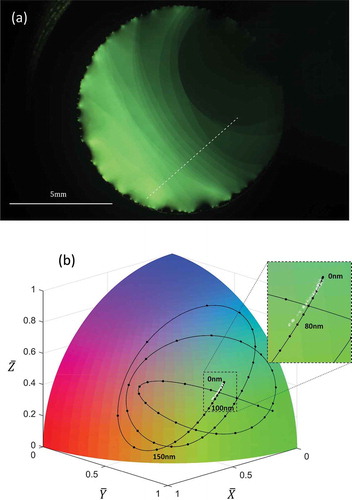
Figure 14. Pixel-wise film thickness plotted against the square root of the pixel-wise reflectivity $R_F$ for $\alpha =1.0$

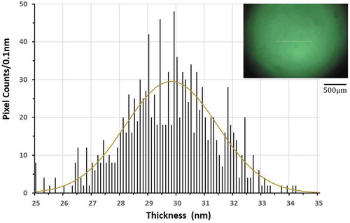
Figure 15 shows the image of a uniform free-standing film after equilibration for over 24 hours and the distribution of pixel-wise thicknesses along the 800$\mu$m-long cross-sectional line at the centre of the film. The total number of pixels is 1207, which is translated to 0.66$\mu$m/pixel. According to the best fit Gaussian curve, the mean value of the thickness is 29.8 nm with the standard deviation of 1.6 nm. Although the error in pixel-wise thickness becomes more pronounced inversely proportional to the thickness as the film thins, the result in Figure 15 demonstrates that statistically meaningful values can be extracted by considering an increasing number of pixels even for thin films consisting of less than 10 smectic layers.

Figure 15. (Colour online) Distribution of pixel-wise thicknesses along the 800$\mu$m-long cross section (broken white line in the inset) indicated as a histogram of pixel counts per 0.1 nm thickness window. The free-standing film of 8CB was equilibrated for over 24 hours to be uniform in thickness, and imaged at 3.0X magnification for 0.42 sec exposure. The average of 10 images was taken to enhance S/N ratio. The brown line shows the best fit Gaussian

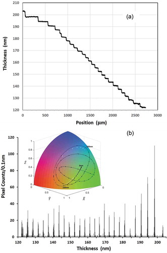
Using $\alpha =1.0$ as determined above, we have analysed thicker films as shown in Figures 16 and 17, where a better accuracy is anticipated. The film consists of multiple terraces, which are decorated with varying colour and intensity. In Figure 16(b), we notice that the plotted data points follow fairly closely the colour trajectory with $\alpha =1.0$. The data points are segregated in isolated spots, corresponding to the individual terraces except for transition areas. In this plot, each data point is plotted as a white circle with 95% transparency to make the contrast reflect the density of the data points. In reference to the colour-thickness trajectory, the thickness of the film at each pixel can be quantitatively estimated by projecting the colour coordinates onto the trajectory. Figure 17 shows the cross-sectional profile of the thickness thus obtained along the broken white line in Figure 16(a). It clearly depicts a step-wise decrease of thickness from left to right along the line. Shown in Figure 17(b) is the histogram of pixels for 0.1 nm window of film thickness. The histogram consists of regularly spaced peaks, each representing the thickness of the film at the terrace. The standard deviation of the thickness values for each peak is less than 0.2 nm in this example, and the layer thickness is on the average 3.10$\pm$0.02 nm, which is in good agreement with the literature values [3,16,24]. It must be noted, however, that the present thickness value is relative to the refractive index assumed in the evaluation of the colour-thickness trajectory. The execution time of the thickness mapping for over 1000 data points is less than 30 sec using the uncompiled MATLAB program running on the modestly powered computer.

Figure 16. (Colour online) (a) Raw image of a free-standing smectic film of 8CB captured at 2.0X magnification and 40 ms exposure time. (b) The colour coordinates of whole pixels plotted as semi-transparent white dots on the colour quadrant along with the colour trajectory. All pixels from the entire image with the intensity higher than 20% of the peak intensity are selected

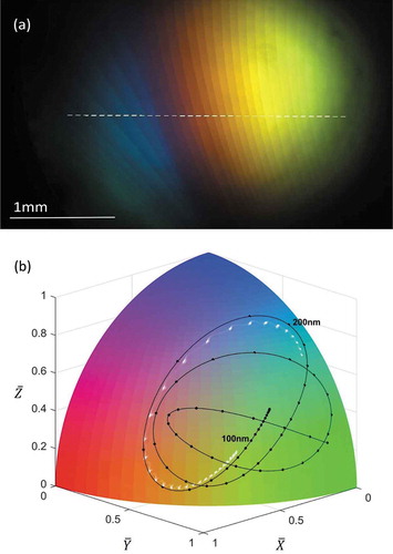
Figure 17. (Colour online) (a) Cross sectional thickness profile along the white broken line in Fig.16(a). (b) Histogram of pixel counts per 0.1 nm window of thickness for the cross section; the inset shows colour coordinates along the cross section plotted on the colour quadrant. The largest and smallest thickness peaks are located at 203.0$\pm$0.2 nm and 122.3$\pm$0.3 nm, respectively, and there are 27 layers. The smectic layer thickness (average spacing between neighbouring peaks) is evaluted to be 3.10$\pm$0.02 nm

Conclusions

We have developed a robust optical technique for rapid mapping of thickness of free-standing smectic films based on the colour information of reflected light from the film. The accuracy of thickness is sufficiently high for moderately thick films over 50 nm to allow thickness mapping with a pixel-by-pixel resolution; yet it is still possible to analyse thicknesses of thinner films by exploiting a statistical mean of a progressively larger number of pixels, or equivalently a larger area of the film. Although the working principle of the method is straightforward and is readily applicable in regular laboratories, the implementation is far from trivial to secure sufficiently high accuracy of the optical characteristics of the optical components involved. In spite of the careful in-house characterisation of the optical system in the present study, it turned out to be necessary to include an adjustable parameter to fine-tune the theoretical reference, particularly near the 0-thickness limit. The absence of absolute 0 thickness point is one of the inherent weaknesses of the method when compared to the standard technique based the reflectivity. To take full advantage of the method, designing a dedicated optical system optimised for this purpose should be feasible and meaningful.

Another improvement that needs to be considered is the incorporation of the effect of optical anisotropy of smectics to expand the application beyond smectic A liquid crystals. In optically anisotropic media, the incident light is split into two eigen modes – ordinary and extraordinary waves [21]. Upon multiple reflections, the two modes are not in general conserved except for the symmetrical case in which the optic axis of the film lies in the plane of incidence [25]. As a result, corresponding to the combination of two eigen modes, there appear multiple colour-thickness trajectories, and the one for a particular incident light for illumination is given by a weighted average of the multiple trajectories. Since the ordinary and the extraordinary waves travel different optical paths in the film, this effect can be qualitatively similar to the case of illumination containing multiple colour components with slightly different wavelengths. We, therefore, anticipate that the method and the procedure described above should essentially apply to optically anisotropic films as well.

The CMOS camera we used had a minute colour shift from one pixel to another. Although this is not problematic in the thick film region, where there is a sufficiently wide margin of accuracy, it becomes one of the most significant sources of error in thinner films. A subsequent work is ongoing to address this issue by characterising the colour filter transmission at the pixel level, not as the average of the whole image sensor as we did in the present study. In terms of the execution time, furthermore, a drastic acceleration is foreseeable by improving the solution algorithm from the current point-wise projection on the colour-thickness trajectory to a direct readout scheme using a prefabricated lookup table. Combined with a more powerful computer and the code compilation, we expect that a real 2D mapping in a reasonable time frame, if not real-time, should become practical.

Disclosure statement

No potential conflict of interest was reported by the author(s).

Additional information

Funding

This study was supported by the National Aeronautics and Space Administration (NASA) under Grant [NNX17AD68G].

References

- de Gennes PG. The Physics of Liquid Crystals. Clarendon Press. Oxford (UK), 1979. ISBN 0198512856, 9780198512851.
- Oswald P, Pieranski P. Smectic and columnar liquid crystals: concepts and physical properties illustrated by experiments. CRC Press, Boca Raton(FL). 2005. ISBN 9780849398407.
- Leadbetter AJ, Frost JC, Gaughan JP, et al. The structure of smectic A phases of compounds with cyano end groups. J Phys France. 1979;40:375–380.
- de Jeu WH, Ostrovskii BI, Shalaginov AN. Structure and fluctuations of smectic membranes. Rev Mod Phys. 2003;75:181–235.
- Young CY, Pindak R, Clark NA, et al. Light-scattering study of two-dimensional molecular-orientation fluctuations in a freely suspended ferroelectric liquid-crystal film. Phys Rev Lett. 1978;40:773.
- Rosenblatt C, Meyer RB, Pindak R, et al. Temperature behavior of ferroelectric liquid-crystal thin films: A classical XY system. Phys Rev A. 1980;21:140.
- Pieranski P, Beliard L, Tournellec JP, et al. Physics of smectic membranes. Phys A. 1993;194:364–389.
- Rosenblatt C, Amer NM. Optical determination of smectic A layer spacing in freely suspended thin films. Appl Phys Lett. 1980;36:432–434.
- Stoebe T, Mach P, Huang CC. Unusual layer-thinning transition observed near the Smectic-A-Isotropic transition in free-standing liquid-crystal films. Phys Rev Lett. 1994;73:1384.
- Mach P, Huang CC, Stoebe T, et al. Surface tension obtained from various smectic free-standing films: the molecular origin of surface tension. Langmuir. 1998;14(15):4330–4341.
- Nguyen ZH, Park CS, Pang J, et al. Surface energetics of freely suspended fluid molecular monolayer and multilayer smectic liquid crystal films. PNAS. 2012;109:12873–12877.
- Dolganov PV, Shuravin NS, Dolganov VK. Coalescence of holes in two-dimensional free-standing smectic films. Phys Rev E. 2020;101:052701.
- Sirota EB, Pershan PS. X-ray and optical studies of the thickness dependence of the phase diagram of liquid-crystal films. Phys Rev A. 1987;36:2890–2901.
- Stannarius R, Trittel T, Klopp C, et al. Freely suspended smectic films with in-plane temperature gradients. New J Phys. 2019;21:063033.
- Kraus I, Pieranski P, Demikhov E, et al. Destruction of a first-order smectic-A→smectic-C* phase transition by dimensional crossover in free-standing films. Phys Rev E. 1993;48:1916–1923.
- Jaquet R, Schneider F. Dependence of film tension on the thickness of smectic films. Phys Rev E. 2003;68:039902.
- Picano F, Oswald P, Kats EI. Disjoining pressure and thinning transitions in smectic-A liquid crystal films. Phys Rev E. 2001;63:021705.
- Schulz B, Mazza MG, Bahr C. Single-molecule diffusion in freely suspended smectic films. Phys Rev E. 2014;90:040501(R.
- Dolganov PV, Kats EI, Dolganov VK. Collapse of islands in freely suspended smectic nanofilms. JETP Lett. 2017;106:229–233.
- Maxwell JC. On the theory of compound colours, and the relations of the colours of the spectrum. Phil Trans Royal Soc. 1860;150:57–84.
- Born M, Wolf E. Principles of Optics. New York: Pergamon Press; 1980. ISBN 0-08-026482-4.
- Ryer A. Light Measurement Handbook. International Light, Newburyport (MA), 1997. http://apps.usd.edu/coglab/schieber/pdf/handbook.pdf
- Jaquet R, Schneider F. Dispersion of the ordinary refractive indices of smectic liquid crystals in free-standing films. Phys Rev E. 2006;74:011708.
- Palermo MF, Muccioli L, Zannoni C. Molecular organization in freely suspended nano-thick 8CB smectic films. An atomistic simulation. Phys Chem Chem Phys. 2015;17:26149–26159.
- Tabe Y, Yokoyama H. Fresnel formula for optically anisotropic Langmuir monolayers: an application to Brewster angle microscopy. Langmuir. 1995;11(3):699–704.