Rapid thickness mapping of free-standing smectic films using colour information of reflected light II: real-time areal mapping using lookup table scheme

ABSTRACT

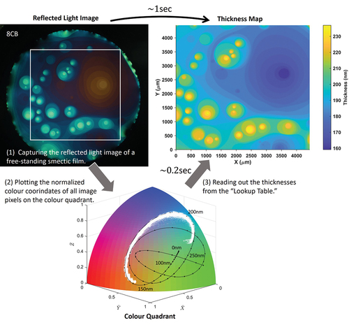
In the previous paper [Liq Cryst. 2020; 48(6): 873–887], we demonstrated that the thickness of free-standing smectic films can be accurately determined from microscopic reflective images, solely utilising the colour information on the image. Even after full vectorisation of the computational code, however, it took ca. 0.1 ms per data point, leaving a big room of improvement to realise a true real-time 2D thickness mapping. Here, we show that the processing speed can be enhanced by a factor of 350 by using a lookup table scheme based on a modified hierarchical triangular partitioning of the colour space. A one-million-pixel image can now be captured and processed in 1 s, offering a clear path to a true video rate 2D thickness mapping.

Graphical abstract

KEYWORDS:

• Triangular mesh
• lookup table
• hierarchical triangular partitioning
• thickness measurement
• free-standing smectic films
• real-time thickness mapping
• reflective images
• MATLAB

Introduction

Free-standing smectic films are a quasi-2D condensed matter system, whose thicknesses can span from two to several hundred molecular layers [1,2]. As a critical physical variable, measurement of the film thickness is always a significant part of the film characterisation [1,3–21]. The existing techniques for thickness measurement are mostly optical, based on the multiple interference of incident light. For thinner films of up to 50 nm, the quadratic dependence of reflection intensity provides an accurate estimate of thickness [3–9]. For thicker films, the observation of the interference spectrum or colour under white light illumination plays a complementary role with a varying degree of precision [1,7,10–13]. In general, the colour has been considered to be less quantitative than the spectral measurement due to insufficient characterisation of illumination and detection conditions. Alternatively, for moderately thick films, the microscopic interferometry using a monochromatic light offers a highly quantitative modality [1,10,12,14–18]. In a previous paper [22], we have demonstrated a rapid and robust thickness mapping method based on the colour information of the reflected light image. It is quantitative and covers the film thickness below 1 μm, and the thickness profile along a cross section consisting of 1000 pixels can be obtained in 30 s with an accuracy better than 1 nm. The present paper, as a sequel of the previous publication, presents orders of magnitude acceleration of thickness mapping by employing a lookup table scheme, in which the thicknesses are preassigned to tiny partitions over the entire colour space and are retrieved on-demand. We show that 2D mapping of the film thickness consisting of one million pixels can be finished in 1 s, which paves the way to a true real-time thickness mapping.

Principle of the colour-based thickness mapping

Only the outline of the method will be given here; for complete details, readers are referred to the previous paper [22]. We observe the reflected image of free-standing films with a high dynamic-range colour camera, which provides the 12-bit colour coordinates $\left(X,Y,Z\right)$ for each pixel corresponding to Red (R), Green (G) and Blue (B) components of reflected light. The intensity information is removed by normalising the colour coordinates onto a unit sphere according to $\left(\bar{X},\bar{Y},\bar{Z}\right)=\left(X,Y,Z\right)/\sqrt{X^2+Y^2+Z^2}$, which makes this method more robust against unavoidable spatial and temporal intensity variations. 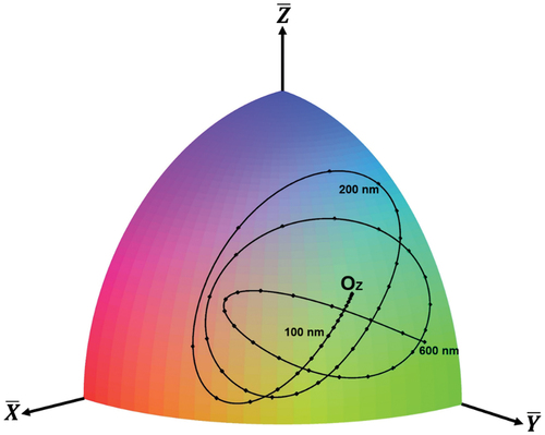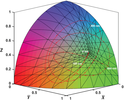Based on the Fresnel formula of multiple reflection from the free-standing film, we can theoretically calculate the normalised colour coordinates as a function of the film thickness $h$ as $\left(\bar{X}\left(h\right),\bar{Y}\left(h\right),\bar{Z}\left(h\right)\right)$ for given conditions of illumination spectrum and the refractive index of the film. It forms a trajectory on the colour space (hereafter referred to as the colour quadrant) as shown in Figure 1. For the observed image, the thickness at a point characterised by the normalised colour coordinates $\left(r_c,g_c,b_c\right)$ is obtained as the thickness $h_c$, where $\left(\bar{X}\left(h_c\right),\bar{Y}\left(h_c\right),\bar{Z}\left(h_c\right)\right)$ gives the closest point to $\left(r_c,g_c,b_c\right)$ on the trajectory. A large part of the computation time, even after full vectorisation in MATLAB, is consumed by this step of finding the point of closest approach on the trajectory.

Figure 1. (Colour online) Colour quadrant and the theoretical thickness-colour trajectory for 8CB(4-octyl-4ʹ-cyanobiphenyl) from 0 nm to 600 nm thickness. $O_z$ stands for the 0-thickness point.

Acceleration by lookup table scheme

Substantial acceleration of computation is, therefore, anticipated if the aforementioned critical step can be replaced by a more efficient computational procedure. Instead of directly calculating the thickness for each observed point, the thicknesses can be retrieved from a lookup table of thicknesses, preassigned based on the closest-to-trajectory method, to small partitions covering the entire colour space. In general, the smaller the partitions become, the more accurate the thicknesses. The obvious requirements for this lookup table scheme to work as expected are as follows: 1) a systematic algorithm to split the colour sphere into partitions that are small enough to guarantee the required accuracy all along the thickness-colour trajectory, and 2) an efficient indexing scheme with the minimum computational load to identify the partition that embraces an arbitrarily given point on the colour sphere.

Partitioning a sphere has a fundamental significance in a wide range of fields from mathematics, computer graphics to Earth science and astronomy [23,24]. The best-known is the latitude-longitude system, which is based on the polar and the azimuthal angles. Despite its intuitive clarity, one of the serious disadvantages is the nonuniformity of the area of partition with the rapid shrinkage of size towards the poles. In recent years, significant progress has been made in splitting the sphere into partitions of similar, if not identical, shape and size [25,26]. For any partitioning scheme to be practically useful, it must provide a simple and systematic protocol to uniquely index the partitions so that any given point on the sphere can be readily associated with the index of the partition that contains the point.

For the present purpose to build a lookup table for thickness mapping, we employ the hierarchical triangular mesh (HTM) partitioning and modify it to suit the present context [25]. The HTM partitioning begins with an octahedron inside a unit sphere having eight vertices at $\left(\pm 1,0,0\right)$, $\left(0,\pm 1,0\right)$ and $\left(0,0,\pm 1\right)$. At the next level of hierarchy, each of the eight equilateral triangles is split into four similar equilateral triangles, and the vertices are projected on the sphere from the origin, resulting in 32 triangular partitions. In the HTM partitioning, the same procedure is recursively applied to all the triangles, generating, after $D$ steps, $2^{2D+3}$ triangular partitions. The triangles are uniquely addressed recursively by means of $D+1$ dimensional indexes. The present colour quadrant, i.e. the positive quadrant of the upper hemisphere, is associated with one equilateral triangle of the octahedron. Therefore, if we are to split the colour quadrant into one million partitions, the required level of hierarchy becomes $D=10$. Although the indexing is systematic, repeating 10 layers of recursive indexing for each data point on the colour quadrant is computationally inefficient.

To alleviate this problem, we depart from the original HTM in the second step as described below. We must note here that in order to guarantee the uniform precision of thicknesses over the entire colour quadrant, the partitions near the 0-thickness point, $O_z$ in Figure 2, should be taken smaller depending on its distance from the 0-thickness point. First, the 0-thickness point is projected from the origin to a point $O$ outside the sphere. The distance between $O$ and the origin is given later. Then, we consider three triangles $OAB$, $OBC$ and $OCA$ where $\mathbf{A}=\left(1,0,0\right)$, $\mathbf{B}=\left(0,1,0\right)$ and $\mathbf{C}=\left(0,0,1\right)$. We split each of these mother triangles into $N^2$ identical child triangles by dividing each side into $N$ segments of equal length as shown in Figure 3. Finally, the triangles on $OAB$, $OBC$ and $OCA$ are projected back on the sphere, generating a spherical partitioning made of $3N^2$ spherical triangles, as shown in Figure 4. Before back-projection, the child triangles on the same mother triangle, say $OAB$, are of the same shape and size; however, the spherical triangles after back-projection have smaller size near the 0-thickness point than at the bottom, i.e. the $AB$ arc, to be compliant with the present requirement. To be more specific, let ${\mathbf{O}}_{\mathrm{z}}=\left({\bar{X}}_z,{\bar{Y}}_z,{\bar{Z}}_z\right)$ and $\alpha$ be the length of $\mathbf{O}=\alpha \left({\bar{X}}_z,{\bar{Y}}_z,{\bar{Z}}_z\right)$ . The normal vector of the triangle $OAB$ is then written as

(1) ${\mathbf{n}}_{AB}=\left(\mathbf{A}-\mathbf{O}\right)\times \left(\mathbf{B}-\mathbf{O}\right)=\alpha {\bar{Z}}_z\left(\mathbf{A}+\mathbf{B}\right)+\left(1-\alpha {\bar{X}}_z-\alpha {\bar{Y}}_z\right)\mathbf{C}$(1)

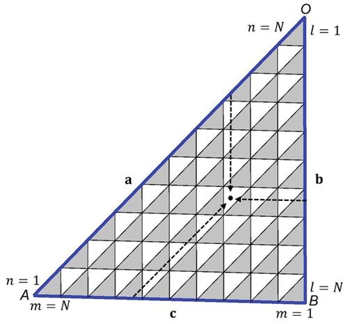
Figure 2. (Colour online) Construct of modified hierarchical triangular partition of the colour quadrant. The equilateral triangle $ABC$ is one of the faces of octahedron, from which the partitioning starts. $O_z$ is the 0-thickness point on the colour quadrant, and the radial line $O_0{O}_z$ is extended by a factor of $\alpha$ to the point $O$. An arbitrary point $P$ on the colour quadrant is radially projected to $Q$, which is on either of the three triangles $OAB$, $OBC$ and $OCA$. In this example, the point $Q$ is on $OAB$, and the line passing $O$ and $Q$ intersects the line $AB$ at the point $E$.

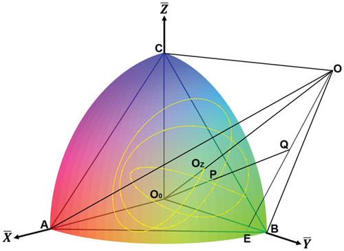
Figure 3. (Colour online) Partitioning the equilateral triangular pyramid $ABCO$ covering the entire colour quadrant. Each face is partitioned into identically shaped child triangles. In this example, $N=10$, and each of $OAB,OBC$and $OCA$ contains $N^2=100$ child triangles.

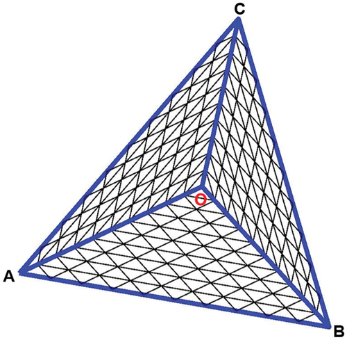
Figure 4. (Colour online) The spherical triangular mesh partitioning the colour quadrant. The red dots on the trajectory indicate 10 nm differences of the thickness. Here we have used $\alpha =4$ and $N=10$ to make the partitions clearly visible relative to the 0-thickness point.

Hence, the areal magnification $\eta$ upon back-projection of the triangle onto the sphere is dependent on the position $\mathbf{P}=\left(\bar{X},\bar{Y},\bar{Z}\right)$ on the colour quadrant and is given by

(2) ${\eta }_{AB}=\frac{{\mathbf{n}}_{AB}.\mathbf{P}}{\left|{\mathbf{n}}_{AB}\right|}=\frac{\alpha {\bar{Z}}_z\left(\bar{X}+\bar{Y}\right)+\left(1-\alpha {\bar{X}}_z-\alpha {\bar{Y}}_z\right)\bar{Z}}{\sqrt{1+{\alpha }^2+2{\alpha }^2{\bar{X}}_z{\bar{Y}}_z-2\alpha \left({\bar{X}}_z+{\bar{Y}}_z\right)}}$(2)

It immediately follows from this equation that at the 0-thickness point, the scaling factor decreases with increasing $\alpha$ as ${\eta }_{AB}\left(O_z\right)\approx {\bar{Z}}_z/\alpha \sqrt{1+2{\bar{X}}_z{\bar{Y}}_z}$, and along the $AB$ arc, it stays finite as ${\eta }_{AB}\left(\breve{AB}\right)\approx {\bar{Z}}_z\left(\bar{X}+\bar{Y}\right)/\sqrt{1+2{\bar{X}}_z{\bar{Y}}_z}$. The ratio ${\eta }_{AB}\left(O_z\right)/{\eta }_{AB}\left(\breve{AB}\right)=\left(\bar{X}+\bar{Y}\right)/\alpha$ is not significantly dependent on the location of the 0-thickness point. In Figures 2–4, we assumed $\alpha =4$ and $N=10$ for the sake of clarity of illustration. In the real applications to be described below, we use $\alpha =10$ and $N=600$.

Indexing the partitions

Indexing partitions is not just numbering the partitions but is a system of addresses that allows us to locate a given partition on the sphere and, conversely, to identify the partition containing a given point on the sphere. We devised an efficient indexing scheme for the present spherical-triangular partitioning, which is compatible with vectorial computation on the MATLAB platform. Let us consider the mother triangle $OAB$ in Figure 5. All sides are split into $N$ segments of equal length, resulting in $N^2$ child triangles of identical shape and size similar to the mother triangle. There are two different types in these triangles: those $N\left(N+1\right)/2$ triangles with the tip pointing up (grey coloured) and those $N\left(N-1\right)/2$ triangles with the tip pointing down (white coloured). We introduce here the row indices $\left(l,m,n\right)$ where $l$ counts the rows parallel to the $AB$ side starting from the vertex $O$, and $m$ and $n$ count the rows parallel to $OA$ and $OB$, respectively. As shown in Figure 5, the child triangle is uniquely specified by $\left(l,m,n\right)$. Although $l,m$ and $n$ run from 1 to $N$, they are not mutually independent but satisfy the following relation:

(3) $l+m+n=\left\{\begin{array}{cc}2N+1& \cdot \cdot \cdot \cdot \cdot \cdot \cdot \cdot \cdot \mathrm{G}\mathrm{r}\mathrm{e}\mathrm{y}\mathrm{T}\mathrm{r}\mathrm{i}\mathrm{a}\mathrm{n}\mathrm{g}\mathrm{l}\mathrm{e}\mathrm{s}\\ 2N+2& \cdot \cdot \cdot \cdot \cdot \cdot \cdot \mathrm{W}\mathrm{h}\mathrm{i}\mathrm{t}\mathrm{e}\mathrm{T}\mathrm{r}\mathrm{i}\mathrm{a}\mathrm{n}\mathrm{g}\mathrm{l}\mathrm{e}\mathrm{s}\end{array}\right..$(3)

Figure 5. (Colour online) Two types of child triangles and the schematic illustration of indexing. $N=10$. The white triangle with a black dot is indexed as $\left(l,m,n\right)=\left(7,7,8\right)$ following the blue arrows from the edges. Note that $l+m+n=22=2N+2$.

Because of this extra constraint, the 3D matrix $\left(l,m,n\right)$ itself is not suitable for efficient matrix operations. We can, however, convert $\left(l,m,n\right)$ to an unconstrained $N\times N$ matrix $\left(m^{\mathrm{\prime }},n^{\mathrm{\prime }}\right)$ by the following rule:

(4) $\begin{array}{rl}& \left.\begin{array}{c}m{ }^{\mathrm{\prime }}=m\\ n{ }^{\mathrm{\prime }}=n\end{array}\right\}\mathrm{w}\mathrm{h}\mathrm{e}\mathrm{n}l+m+n=2N+1,\\ & \left.\begin{array}{c}m{ }^{\mathrm{\prime }}=N-m+1\\ n{ }^{\mathrm{\prime }}=N-n+1\end{array}\right\}\mathrm{w}\mathrm{h}\mathrm{e}\mathrm{n}l+m+n=2N+2.\end{array}$(4)

In the former case, $m{ }^{\mathrm{\prime }}+n{ }^{\mathrm{\prime }}\ge N+1$, and in the latter, $m{ }^{\mathrm{\prime }}+n{ }^{\mathrm{\prime }}\le N$. The inverse conversion from $\left(m^{\mathrm{\prime }},n^{\mathrm{\prime }}\right)$ to $\left(l,m,n\right)$ is given by

(5) $\begin{array}{rl}& \left.\begin{array}{c}l=2N+1-m{ }^{\mathrm{\prime }}-n\mathrm{\prime }\\ m=m{ }^{\mathrm{\prime }}\\ n=n{ }^{\mathrm{\prime }}\end{array}\right\}\mathrm{w}\mathrm{h}\mathrm{e}\mathrm{n}m{ }^{\mathrm{\prime }}+n{ }^{\mathrm{\prime }}\ge N+1,\\ & \left.\begin{array}{c}l=m{ }^{\mathrm{\prime }}+n\mathrm{\prime }\\ m=N-m^{\mathrm{\prime }}+1\\ n=N-n^{\mathrm{\prime }}+1\end{array}\right\}\mathrm{w}\mathrm{h}\mathrm{e}\mathrm{n}m{ }^{\mathrm{\prime }}+n{ }^{\mathrm{\prime }}\le N.\end{array}$(5)

Note that $\left(l,m,n\right)\iff \left(m{ }^{\mathrm{\prime }},n^{\mathrm{\prime }}\right)$ is a one-to-one mapping.

The three mother triangles $OAB$, $OBC$ and $OCA$ are partitioned into $3N^2$ child triangles in total. Concatenating laterally these three $N\times N$ matrices, we obtain an unconstrained $N\times 3N$ matrix, each element of which corresponds to a particular child triangular partition and holds the thickness value at the partition on the colour quadrant. The concatenated matrix $(m{ }^{\mathrm{\prime }\mathrm{\prime }},n{ }^{\mathrm{\prime }\mathrm{\prime }})$ is indexed such that

(6) $\begin{array}{rl}& m{ }^{\mathrm{\prime }\mathrm{\prime }}=m{ }^{\mathrm{\prime }},\\ & n{ }^{\mathrm{\prime }\mathrm{\prime }}=\left\{\begin{array}{c}n{ }^{\mathrm{\prime }}\mathrm{f}\mathrm{o}\mathrm{r}OAB\\ n{ }^{\mathrm{\prime }}+N\mathrm{f}\mathrm{o}\mathrm{r}OBC\\ n{ }^{\mathrm{\prime }}+2N\mathrm{f}\mathrm{o}\mathrm{r}OCA\end{array}\right..\end{array}$(6)

Identifying the partition for a data point

Finally, it is necessary to establish a procedure to find the index of the partition containing an arbitrary data point. Let us consider a point $\mathbf{P}=\left(\bar{X},\bar{Y},\bar{Z}\right)$ on the colour quadrant as illustrated in Figure 2. Radially extending $\mathbf{P}$ to the mother triangles, we obtain the point $\mathbf{Q}=\beta \mathbf{P}$ where $\beta$ is a positive scaling factor. We assume that the point $\mathbf{Q}$ is on the triangle $OAB$. Then, using the normal vector ${\mathbf{n}}_{AB}$ given in Equation (1)(1) ${\mathbf{n}}_{AB}=\left(\mathbf{A}-\mathbf{O}\right)\times \left(\mathbf{B}-\mathbf{O}\right)=\alpha {\bar{Z}}_z\left(\mathbf{A}+\mathbf{B}\right)+\left(1-\alpha {\bar{X}}_z-\alpha {\bar{Y}}_z\right)\mathbf{C}$(1) , we obtain

(7) $\beta =\frac{{\mathbf{n}}_{AB}.\mathbf{O}}{{\mathbf{n}}_{AB}.\mathbf{P}}.$(7)

It is worth noting that we can also formally calculate the scaling factor for $OBC$ and $OCA$:

(7’) $\beta =\frac{{\mathbf{n}}_{BC}.\mathbf{O}}{{\mathbf{n}}_{BC}.\mathbf{P}},\beta =\frac{{\mathbf{n}}_{CA}.\mathbf{O}}{{\mathbf{n}}_{CA}.\mathbf{P}}$(7’)

The mother triangle, on which we actually find the point $\mathbf{Q}$, is the one associated with the smallest positive $\beta$. Although this property can be used to identify the mother triangle for a data point, we can readily confirm from the fact that all the points are in the positive quadrant that there exists a more concise set of conditions for this purpose as follows:

(8) $P\in \left\{\begin{array}{c}OABwhen\frac{P_x}{O_x},\frac{P_y}{O_y}\ge \frac{P_z}{O_z}\\ OBCwhen\frac{P_y}{O_y},\frac{P_z}{O_z}\ge \frac{P_x}{O_x}\\ OCAwhen\frac{P_z}{O_z},\frac{P_x}{O_x}\ge \frac{P_y}{O_y}\end{array}\right.$(8)

Next, to obtain the index of the child triangle, in which $\mathbf{Q}$ is located, we consider the point $\mathbf{E}$ at the intersection of the $AB$ side and the line passing $\mathbf{O}$ and $\mathbf{Q}$. We define a scaling factor $\gamma$ by

(9) $\mathrm{E}-\mathrm{O}={\gamma }_{\mathrm{A}\mathrm{B}}(\mathrm{Q}-\mathrm{O})$(9)

Noting a geometrical identity $\left(\mathbf{A}-\mathbf{O}\right)\times \left(\mathbf{B}-\mathbf{O}\right)=\left(\mathbf{E}-\mathbf{O}\right)\times \left(\mathbf{B}-\mathbf{A}\right)$ and Equations (1)(1) ${\mathbf{n}}_{AB}=\left(\mathbf{A}-\mathbf{O}\right)\times \left(\mathbf{B}-\mathbf{O}\right)=\alpha {\bar{Z}}_z\left(\mathbf{A}+\mathbf{B}\right)+\left(1-\alpha {\bar{X}}_z-\alpha {\bar{Y}}_z\right)\mathbf{C}$(1) and (7(7) $\beta =\frac{{\mathbf{n}}_{AB}.\mathbf{O}}{{\mathbf{n}}_{AB}.\mathbf{P}}.$(7) ), we obtain

(10) ${\gamma }_{AB}=\frac{{\mathbf{n}}_{AB}.{\mathbf{n}}_{AB}}{\left(\frac{{\mathbf{n}}_{AB}.\mathbf{O}}{{\mathbf{n}}_{AB}.\mathbf{P}}\mathbf{P}-\mathbf{O}\right).\left(\mathbf{B}-\mathbf{A}\right)\times {\mathbf{n}}_{AB}}$(10)

Similarly, the scaling factors ${\gamma }_{OA}$ and ${\gamma }_{BO}$ with respect to the $OA$ and $BO$ sides can also be obtained as in Equation (10)(10) ${\gamma }_{AB}=\frac{{\mathbf{n}}_{AB}.{\mathbf{n}}_{AB}}{\left(\frac{{\mathbf{n}}_{AB}.\mathbf{O}}{{\mathbf{n}}_{AB}.\mathbf{P}}\mathbf{P}-\mathbf{O}\right).\left(\mathbf{B}-\mathbf{A}\right)\times {\mathbf{n}}_{AB}}$(10) . Since the mother triangle is split into $N$ rows parallel to the sides, it follows from Equation (10)(10) ${\gamma }_{AB}=\frac{{\mathbf{n}}_{AB}.{\mathbf{n}}_{AB}}{\left(\frac{{\mathbf{n}}_{AB}.\mathbf{O}}{{\mathbf{n}}_{AB}.\mathbf{P}}\mathbf{P}-\mathbf{O}\right).\left(\mathbf{B}-\mathbf{A}\right)\times {\mathbf{n}}_{AB}}$(10) that the index $\left(l,m,n\right)$ for the child triangle we are after is given by

(11) $\left(l,m,n\right)=\left(\left[\frac{N}{{\gamma }_{AB}}\right]+1,\left[\frac{N}{{\gamma }_{OA}}\right]+1,\left[\frac{N}{{\gamma }_{BO}}\right]+1\right)$(11)

where $\left[x\right]$ is the largest integer not exceeding $x$. Equations (10)(10) ${\gamma }_{AB}=\frac{{\mathbf{n}}_{AB}.{\mathbf{n}}_{AB}}{\left(\frac{{\mathbf{n}}_{AB}.\mathbf{O}}{{\mathbf{n}}_{AB}.\mathbf{P}}\mathbf{P}-\mathbf{O}\right).\left(\mathbf{B}-\mathbf{A}\right)\times {\mathbf{n}}_{AB}}$(10) and (11(11) $\left(l,m,n\right)=\left(\left[\frac{N}{{\gamma }_{AB}}\right]+1,\left[\frac{N}{{\gamma }_{OA}}\right]+1,\left[\frac{N}{{\gamma }_{BO}}\right]+1\right)$(11) ) provide the mapping $\mathbf{P}\Rightarrow \left(l,m,n\right)$.

Generating the lookup table and linear indexing

The last step is to assign the thickness values to all the partitions generated. We select the centre of mass of child triangle before back-projection as the representative point for thickness evaluation. Consider the mother triangle $OAB$, and let $\mathbf{a}=\mathbf{A}-\mathbf{O}$ and $\mathbf{b}=\mathbf{B}-\mathbf{O}$. Based on the definition of the index $\left(l,m,n\right)$, it is readily shown that the vector $\mathbf{r}\left(l,m,n\right)$ from the vertex $\mathbf{O}$ to the centre of mass of child triangle $\left(l,m,n\right)$ is written as

(12) $\mathbf{r}\left(l,m,n\right)=\left\{\begin{array}{c}\frac{N-n}{N}a+\frac{N-m}{N}b+\frac{\mathbf{a}+\mathbf{b}}{3N}whenl+n+m=2N+1\\ \frac{N-n}{N}a+\frac{N-m}{N}b+2\frac{\mathbf{a}+\mathbf{b}}{3N}whenl+n+m=2N+2\end{array}\right.$(12)

Projecting the centre of mass onto the colour quadrant, the colour coordinates for evaluation of the thickness for the partition is given by

(13) $\mathbf{x}\left(l,m,n\right)=\frac{\mathbf{r}\left(l,m,n\right)+\mathbf{O}}{\left|\mathbf{r}\left(l,m,n\right)+\mathbf{O}\right|}$(13)

The thicknesses for $\mathbf{x}\left(l,m,n\right)$ for all $\left(l,m,n\right)$ have been evaluated with the least-distance-to-trajectory method as done in the previous paper. In view of the error tolerance better than 1 nm, we adopted $N=600$ resulting in $3N^2=1080000$ partitions. For efficient table lookup processes, the $N\times 3N$ matrix has been further converted to a linear array on MATLAB. The array begins at $\left(1,1\right)$, moves downward the column and jumps to the top of the next column until the $3N$ columns are exhausted. The linear index $k$ runs from 1 to $3N^2$ and is related to the original 2D index by

(14) $k=m{ }^{\mathrm{\prime }\mathrm{\prime }}+N\left(n{ }^{\mathrm{\prime }\mathrm{\prime }}-1\right)$(14)

Given in Figure 6 is the summary of indexing scheme and the lookup table operation. All the equations written in vector forms provide the basis for efficient MATLAB codes.

Figure 6. Schematic summary of indexing, lookup table and lookup steps of data points. The lookup table $\left(k\right)$ is generated following the upper steps from the partitioning of the mother triangles. The colour data point $\mathbf{P}$ is analysed following the lower steps to obtain the corresponding linear index $k$, which is looked up in the lookup table to obtain the thickness $h\left(\mathbf{P}\right)$.

Results and discussions

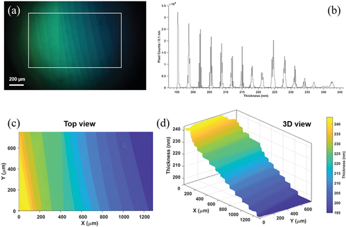
The lookup table scheme has been implemented on MATLAB platform running on a Windows 10 computer (XPS 8930, Dell). Free-standing smectic films of 8CB (4-octyl-4′-cyanobiphenyl) were prepared at 21°C in the airtight film chamber, the details of which include the optical system have been described in the previous paper [22]. Figure 7 shows a 2D thickness map obtained by using the lookup table scheme. The number of data points is approximately 950,000, and it took ca. 2s including the time for image acquisition, 3D rendering, etc. The computation time for the lookup process was 170 ms. The thickness map is colour-coded and indicates clear terraces of the smectic layers. The thickness histogram, Figure 7(b), demonstrates a satisfactory level of accuracy, comparable to the previous results based on direct calculations, yielding the average layer thickness 3.17 ± 0.01 nm.

Figure 7. (Colour online) (a) Reflected image of free-standing smectic film at 4.0$\times$ magnification. (b) Histogram of thickness for 0.1 nm for nearly one million pixels within the rectangular region in (a). The average layer thickness calculated from this result is 3.17 ± 0.01 nm. (c) Top view of the thickness profile for the selected rectangular region in (a). (d) 3D view of the thickness profile.

In order to quantify the improvement of computational efficiency made by the lookup table scheme, we have examined the execution time of the thickness determination routine for a wide range of data sizes. The results shown in Figure 8 indicate that the lookup table scheme always outperforms the direct calculation. While the execution time of the direct calculation increases linearly with the data size over 10,000, that of the lookup table scheme increases much more slowly. The lookup table scheme becomes increasingly more advantageous for larger data sets. For one-million-pixel data, the lookup table scheme takes only 150 ms to complete, compared to 50 s for direct calculations. At this point, the lookup table is 350 times faster, and the advantage grows further as the data size increases. In the present MATLAB code, the overhead time for I/O processing, such as image acquisition from the camera and data transfer between hard drives, is about 1.5 s. Therefore, even at one-million-pixel data size, the CPU execution time is still a minor contribution in the case of the lookup table scheme. Less than 2 s of total processing time per one full-size image makes the present method practically suitable for quasi-real-time thickness mapping of large images.

Figure 8. CPU execution time for thickness calculation as a function of the number of data points.

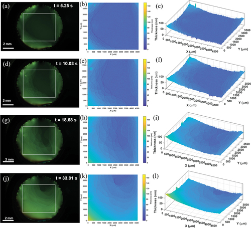
In addition to batch processing of captured images, we explored a free-run mode, in which the image is sequentially captured, analysed for thickness, and converted to a video frame in AVI format. The thickness map is also simultaneously converted to a video. Shown in Figure 9 is an example of the simultaneous image-thickness video for a free-standing film that is under a rapid evolution right after preparation. The data size for thickness mapping is 541,728 pixels. The frame rate is automatically determined at the maximum possible value, which is presently 1.13 fps. The advances of the layer steps towards the centre are clearly visible, particularly in the top-view of thickness map, Figure 9(b,e,h,k). The full video of the image and the thickness map are available as Supplemental Material.

Figure 9. (Colour online) Series of snapshots extracted from the AVI video of free-standing smectic film captured in the free-run mode at 0.7$\times$ magnification: (a) t = 5.25 s, (d) t = 10.03 s, (g) t = 18.68 s, and (j) t = 33.81 s. Top view (b, e, h, and k) and 3D view (c, f, i, and l) of the thickness map for images on the left. The full video is available as Supplemental Material.

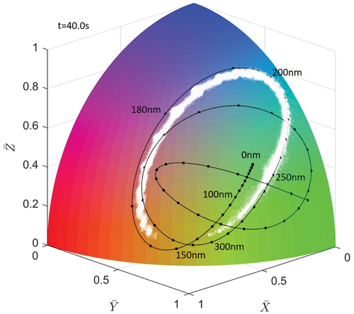
We also tested the free-run mode for a thicker film (150–300 nm) undergoing a rapid structural change after a sudden deflation of the film, held in the bubble shape, with the release of air-pressure difference across the film [19–21]. The abrupt reduction of film area results in nucleation of thicker islands, followed by a rapid process of equilibration. Figure 10 shows a series of snapshots captured at 1.13 fps (the full video is available as Supplemental Material). It is clearly demonstrated that the rapid change in the free-standing film can be faithfully traced in the real-time thickness map. As shown in Figure 10, the interference colour of the reflected image in this range of thickness is not easily relatable to the thickness of the film because of the higher sensitivity of colour to thickness in this range. The possibility to follow the thickness variations in-situ provides a powerful tool to infer the physical behaviours on the spot. Figure 11 shows an example of the distribution of the data points plotted on the colour quadrant, which is playing a background role in the present method. The majority of data points fall in the sufficient vicinity of the thickness-colour trajectory as required. However, when the data points are close to the points of intersection of the trajectory with itself, a caution must be exercised to select the correct portion of the trajectory.

Figure 10. (Colour online) Series of snapshots extracted from the AVI video of relatively thick free-standing smectic film immediately after the sudden deflation. Captured in the free-run mode at 1.13 fps. (a) & (b) t = 40.0 s, (c) & (d) t = 92.7 s, (e) & (f) t = 90.2 s, and (g) & (h) t = 182.4 s. (a, c, e, g) Reflected microscopic images. (b, d, f, h) Top views of thickness map. The full video is available as Supplemental Material.

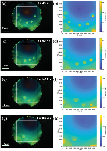
Figure 11. (Colour online) Distribution of data points (white dots) on the colour quadrant for the free-standing film shown in Figure 10(a) with t = 40.0s.

Conclusions

By extending the hierarchical triangular mesh (HTM) partitioning of the sphere, we constructed an algorithm for partitioning the colour quadrant into spherical triangular partitions. The areas of partitions are optimally adjusted to suit the characteristics of the thickness-colour trajectory in such a way as to guarantee the desired accuracy of thickness values everywhere. By selecting $N=600$ segmentation, which results in 1,080,000 partitions in total, enabling an accuracy better than 1 nm, we implemented the lookup table scheme on MATLAB and demonstrated that the CPU execution time of one-million-pixel image is less than 200 ms even on a moderate power desktop computer. This is 350 times acceleration of processing speed compared to the previous system based on the direct calculation of thicknesses using the otherwise identical computational system. This performance allowed a quasi-real-time video observation of reflected images and simultaneously created thickness maps. It is now readily foreseeable that a real video-rate thickness mapping is practically possible by simply employing a more powerful workstation.

We wish to emphasise that the application of the colour-based thickness mapping is not limited to the analysis of free-standing smectic films. It should universally offer an alternative approach to a variety of interferometric techniques that are traditionally reliant on counting the interference fringes [27–29]. The principle of the colour-based technique we presented in a series of papers is not essentially new but has been known for more than a century; however, the colour has been traditionally considered difficult to quantify, not to mention the work of Goethe [30]. We presented here a piece of evidence that the advanced imaging and optical devices, now widely available, enable us to recognise the colour with an unprecedented detail that has never been exploited. In view of the vast range of potential applications, we believe it will lead to a resurgence of colourimetry in a modern outlook [31].

Disclosure statement

No potential conflict of interest was reported by the author(s).

Additional information

Funding

This study was supported by the National Aeronautics and Space Administration (NASA) under Grant NNX17AD68G.

References

- Pieranski P, Beliard L, Tournellec JP, et al. Physics of smectic membranes. Phys A. 1993;194:364–389.
- de Jeu WH, Ostrovskii BI, Shalaginov AN. Structure and fluctuations of smectic membranes. Rev Mod Phys. 2003;75:181–235.
- Young CY, Pindak R, Clark NA, et al. Light-scattering study of two-dimensional molecular-orientation fluctuations in a freely suspended ferroelectric liquid-crystal film. Phys Rev Lett. 1978;40:773.
- Rosenblatt C, Amer NM. Optical determination of smectic A layer spacing in freely suspended thin films. Appl Phys Lett. 1980;36:432–434.
- Mach P, Huang CC, Stoebe T, et al. Surface tension obtained from various smectic free-standing films: the molecular origin of surface tension. Langmuir. 1998;14(15):4330–4341.
- Stoebe T, Mach P, Huang CC. Unusual layer-thinning transition observed near the smectic-A-isotropic transition in free-standing liquid-crystal films. Phys Rev Lett. 1994;73:1384–1387.
- Jaquet R, Schneider F. Dependence of film tension on the thickness of smectic films. Phys Rev E. 2003;68:039902.
- Nguyen ZH, Park CS, Pang J, et al. Surface energetics of freely suspended fluid molecular monolayer and multilayer smectic liquid crystal films. PNAS. 2012;109:12873–12877.
- Qi Z, Ferguson K, Sechrest Y, et al. Active microrheology of smectic membranes. Phys Rev E. 2017;95(1):022702.
- Stannarius R, Trittel T, Klopp C, et al. Freely suspended smectic films with in-plane temperature gradients. New J Phys. 2019;21:063033.
- Schüring H, Stannarius R. Isotropic droplets in thin free standing smectic films. Langmuir. 2002;18:9735–9743.
- Aksenov V, Bläsing J, Stannarius R, et al. Strain-induced compression of smectic layers in free-standing liquid crystalline elastomer films. Liq Cryst. 2005;7:805–813.
- Eremin A, Baumgarten S, Harth K, et al. Two-dimensional microrheology of freely suspended liquid crystal films. Phys Rev Lett. 2011;107:268301.
- Loudet JC, Dolganov PV, Patricio P, et al. Undulation instabilities in the meniscus of smectic membranes. Phys Rev Lett. 2011;106:11802.
- Harth K, Stannarius R. Corona patterns around inclusions in Freely suspended smectic films. Eur Phys J E. 2009;28:265–272.
- Harth K, Schulz B, Bahr C, et al. Atomic force microscopy of menisci of free-standing smectic films. Soft Matter. 2011;7:7103–7111.
- Klopp C, Trittel T, Stannarius R. Self similarity of liquid droplet coalescence in quasi-2D free standing liquid-crystal film. Soft Matter. 2020;16:4607–4614.
- Trittel T, Harth K, Klopp C, et al. Marangoni flow in freely suspended liquid films. Phys Rev Lett. 2019;122:234501.
- Caillier F, Oswald P. Collapse dynamics of smectic-A bubbles. Eur Phys J E. 2006;20:159–172.
- May K, Harth K, Trittel T, et al. Dynamics of freely floating smectic bubbles. Europhys Lett. 2012;100:16003.
- May K, Harth K, Trittel T, et al. Freely floating smectic films. ChemPhysChem. 2013;15:1508–1518.
- Chen W, Yokoyama H. Rapid thickness mapping of free-standing smectic films using colour information of reflected light. Liq Cryst. 2020;48(6):873–887.
- Sahr K, White D, Jon Kimerling A. Geodesic discrete global grid systems. Cartography Geog Inf Sci. 2003;30(2):121–134.
- Gyorgy F. Rendering and managing spherical data with sphere quadtrees. Proceedings of the First IEEE Conference on Visualization: Visualization `90; 1990 Oct 23-26; San Francisco, CA, USA: IEEE, p. 176–186. DOI: https://doi.org/10.1109/VISUAL.1990.146380.
- Szalay A, Gray J, Fekete G, et al. Indexing the Sphere with the Hierarchical Triangular Mesh. Baltimore: The Johns Hopkins University; San Francisco: Microsoft Research Bay Area Research Center; Geneva: CERN; 2005. (MSR-TR-2005-123). Available from: https://arxiv.org/ftp/cs/papers/0701/0701164.pdf
- Rilee M, Kuo K, Clune T, et al. Addressing the big-earth-data variety challenge with the hierarchical triangular mesh. 2016 IEEE International Conference on Big Data (Big Data); 2016 Dec 5-8; Washington, DC, USA: IEEE; p. 1006–1011. DOI: https://doi.org/10.1109/BigData.2016.7840700.
- van der Veen CA, Tran T, Lohse D, et al. Direct measurements of air layer profiles under impacting droplets using high-speed color interferometry. Phys Rev E. 2012;85:026315.
- de Ruiter J, Mugele F, van den Ende D. Air cushioning in droplet impact. I. Dynamics of thin films studied by dual wavelength reflection interference microscopy. Phys Fluids. 2015;27:012104.
- de Ruiter J, Mugele F, van den Ende D. Air cushioning in droplet impact. II. Experimental characterization of the air film evolution. Phys Fluids. 2015;27:012105.
- Charles Lock Eastlake RA. F.R.S., Goethe’s theory of colours: translated from the German. London:John Murray; 1840. Available from: https://archive.org/details/goethestheoryco01goetgoog/page/n6/mode/2up?view=theater.
- Maxwell JC. On the theory of compound colours, and the relations of the colours of the spectrum. Phil Trans Royal Soc. 1860;150:57–84.