A predictive theoretical model for stretch-induced instabilities in liquid crystal elastomers

ABSTRACT

Following the experimental lead, we construct a general mathematical model which, depending on whether the uniaxial scalar order parameter is constant or not, can predict either the classical shear striping instability or the molecular auxetic response and mechanical Fréedericksz transition observed in different liquid crystal elastomers. Our theoretical model can shed some light on the role of nematic order in these stretch-induced mechanical instabilities not observed in conventional rubber-like solids.

Graphical abstract

KEYWORDS:

• Liquid crystal elastomer
• mathematical modelling
• non-linear elasticity
• large strain deformation
• auxeticity
• shear striping

1. Introduction

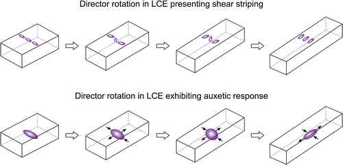
In Refs [1–6], experimental observations are reported for a nematic liquid crystal elastomer (LCE) where an auxetic response occurs, such that, when a material sample is stretched longitudinally, its volume remains unchanged, but its thickness, measured in the direction perpendicular to the sample’s plane, first decreases, then increases if the deformation is sufficiently large. This behaviour is accompanied by a mechanical Fréedericksz transition whereby the nematic director, which is initially aligned within the sample’s plane and perpendicular to the longitudinal direction, is mechanically deformed to become parallel to the applied force. Experimentally, this can appear as a sudden rotation of the director, and is different from the gradual rotation occurring in many other LCEs where alternating shear stripes form at very low stress [7–13]. Discontinuous rotation of the nematic director was also reported previously by Mitchell et al. [14] (see [15, Section 5.5]).

While the shear-striping phenomenon in nematic LCEs is well understood and has been modelled extensively [8,16–24], auxetic LCEs require more physical and theoretical investigation.

In Mihai et al. [25], a descriptive three-term Ogden-type model [26,27] is adopted which permits the calibration to available experimental data for the auxetic LCE. However, despite the inherent mathematical simplicity of the Ogden strain-energy function, fewer terms are needed in order to assess the effect of changing parameter values.

In this paper, guided by experimental observations, we propose a two-term Ogden-type constitutive model, introduced in Section 2, which, depending on whether the uniaxial scalar order parameter is constant or not, predicts either the auxetic response and the mechanical Fréedericksz transition (Section 2.1) or the classical shear striping (Section 2.2) presented by various LCEs (see Figure 1). These results are illustrated by a set of examples presented in Section 3.

Figure 1. (Colour online) Deformation-dependent director rotation leading to alternating shear stripes or large-strain auxetic response in LCEs [28].

2. Model function

We consider the following two-term strain-energy function describing a nematic LCE (see also [25]),

(1) $W^{(lce)}=\frac{{\mu }_1}{2n^2}\left({\lambda }_1^{2n}+{\lambda }_2^{2n}+{\lambda }_3^{2n}\right)+\frac{{\mu }_2}{2n^2}\left({\alpha }_1^{-2n}+{\alpha }_2^{-2n}+{\alpha }_3^{-2n}\right),$(1)

where ${\mu }_1>0$, ${\mu }_2>0$ and $n>0$ are constant parameters, and $\mu ={\mu }_1+{\mu }_2$ represents the shear modulus at infinitesimal strain. In the above equation, $\{{\lambda }_1^2,{\lambda }_2^2,{\lambda }_3^2\}$ denote the eigenvalues of the Cauchy–Green tensor $\mathbf{F}{\mathbf{F}}^T$, where $\mathbf{F}$ is the deformation gradient from the reference cross-linking state, and $\{{\alpha }_1^2,{\alpha }_2^2,{\alpha }_3^2\}$ are the eigenvalues of $\mathbf{A}{\mathbf{A}}^T$, where $\mathbf{A}={\mathbf{G}}^{-1}\mathbf{F}{\mathbf{G}}_0$ is the local elastic deformation tensor, with ${\mathbf{G}}_0$ and $\mathbf{G}$ the ‘natural’ deformation tensors due to the liquid crystal director in the reference and current configuration, respectively. These tensors satisfy the following relations [29] (see also [15, Chapter 3]):

(2) ${\mathbf{G}}_0^2=c_0\left(\mathbf{I}+2{\mathbf{Q}}_0\right),{\mathbf{G}}^2=c\left(\mathbf{I}+2\mathbf{Q}\right),$(2)

with $c_0$ and $c$ representing the effective step length of the polymeric chain, ${\mathbf{Q}}_0$ and $\mathbf{Q}$ the symmetric traceless order parameter tensors [15, pp.48-49], and $\mathbf{I}=\mathrm{d}\mathrm{i}\mathrm{a}\mathrm{g}(1,1,1)$ the tensor identity. The macroscopic tensor parameters are known to describe orientational order in nematic liquid crystals [30].

In the following sections, we demonstrate that, for a suitable choice of the constitutive parameters, the model defined by (1) is capable of predicting either a large-strain auxetic response accompanied by mechanical Fréedericksz transition or the shear-striping instability.

2.1. Variable order parameter and mechanical Fréedericksz transition

First, we examine the emergence of large-strain auxetic behaviour. To obtain this, for the LCE sample, in a Cartesian system of coordinates $(X_1,X_2,X_3)$, we designate the plane formed by the first two directions as the sample’s plane and the third direction as its thickness direction. The material sample is elastically deformed by application of a tensile force in the first (longitudinal) direction, while the nematic director is initially along the second (transverse) direction.

Setting the nematic director in the reference and current configuration, respectively, as follows:

(3) ${\mathbf{n}}_0=\left[\begin{array}{c}0\\ 1\\ 0\end{array}\right],\mathbf{n}=\left[\begin{array}{c}sin\theta \\ cos\theta \\ 0\end{array}\right],$(3)

where $\theta \in [0,\pi /2]$ is the angle between $\mathbf{n}$ and ${\mathbf{n}}_0$, the deformation gradient takes the form

(4) $\mathbf{F}=\mathrm{d}\mathrm{i}\mathrm{a}\mathrm{g}({\lambda }_1,{\lambda }_2,{\lambda }_3),$(4)

with ${\lambda }_1{\lambda }_2{\lambda }_3=1$ and $\mathrm{d}\mathrm{i}\mathrm{a}\mathrm{g}(\cdot ,\cdot ,\cdot )$ denoting a diagonal second-order tensor.

Guided by experimental observations (see also [24]), we assume that the rotation of the nematic director within the plane formed by its initial orientation and the applied force from $\theta =0$ to $\theta =\pi /2$ happens suddenly [25], and denoted by ${\lambda }_{crt}$ the longitudinal stretch ratio $\lambda$ where the rotation occurs. In practice, although the angle $\theta$ will also take intermediate values between $0$ and $\pi /2$, the deformation interval for which the director rotation is observed is very short, and its separate analysis can be omitted. However, in this case, a jump may be observed in the orthogonal stretch ratios ${\lambda }_2$ and ${\lambda }_3$ at the critical longitudinal stretch ${\lambda }_1={\lambda }_{crt}$.

In the reference configuration, the LCE is uniaxial, and the order parameter tensor is equal to [15, p. 14]

(5) ${\mathbf{Q}}_0=\mathrm{d}\mathrm{i}\mathrm{a}\mathrm{g}\left(-\frac{Q_0}{2},Q_0,-\frac{Q_0}{2}\right),$(5)

where $Q_0$ is the scalar order parameter.

In the deformed configuration, biaxiality can also emerge [15, p. 15], and therefore

• If $\theta =0$, then the order parameter tensor takes the form

(6) $\mathbf{Q}=\mathrm{d}\mathrm{i}\mathrm{a}\mathrm{g}\left(-\frac{Q-b}{2},Q,-\frac{Q+b}{2}\right);$(6)

• If $\theta =\pi /2$, then

(7) $\mathbf{Q}=\mathrm{d}\mathrm{i}\mathrm{a}\mathrm{g}\left(Q,-\frac{Q-b}{2},-\frac{Q+b}{2}\right),$(7)

where $Q$ and $b$ are the uniaxial and biaxial scalar order parameters, respectively.

Numerically, we will consider both the cases when biaxiality is neglected, i.e. $b=0$, and when the magnitude of biaxial parameter $b$ increases (decreases) as the uniaxial order parameter decreases (increases).

For the corresponding elastic Cauchy–Green tensor ${\mathbf{A}}^T\mathbf{A}=\mathrm{d}\mathrm{i}\mathrm{a}\mathrm{g}\left({\alpha }_1^2,{\alpha }_2^2,{\alpha }_3^2\right)$, where $‘‘T\prime \prime$ denotes the transpose (see also [25]), we have

• If $\theta =0$, then

(8) ${\alpha }_1^2={\left[\frac{det\left(\mathbf{I}+2\mathbf{Q}\right)}{det\left(\mathbf{I}+2{\mathbf{Q}}_0\right)}\right]}^{1/3}\frac{1-Q_0}{1-(Q-b)}{\lambda }_1^2,$(8)

(9) ${\alpha }_2^2={\left[\frac{det\left(\mathbf{I}+2\mathbf{Q}\right)}{det\left(\mathbf{I}+2{\mathbf{Q}}_0\right)}\right]}^{1/3}\frac{1+2Q_0}{1+2Q}{\lambda }_2^2,$(9)

(10) ${\alpha }_3^2={\left[\frac{det\left(\mathbf{I}+2\mathbf{Q}\right)}{det\left(\mathbf{I}+2{\mathbf{Q}}_0\right)}\right]}^{1/3}\frac{1-Q_0}{1-(Q+b)}{\lambda }_3^2;$(10)

• If $\theta =\pi /2$, then

(11) ${\alpha }_1^2={\left[\frac{det\left(\mathbf{I}+2\mathbf{Q}\right)}{det\left(\mathbf{I}+2{\mathbf{Q}}_0\right)}\right]}^{1/3}\frac{1-Q_0}{1+2Q}{\lambda }_1^2,$(11)

(12) ${\alpha }_2^2={\left[\frac{det\left(\mathbf{I}+2\mathbf{Q}\right)}{det\left(\mathbf{I}+2{\mathbf{Q}}_0\right)}\right]}^{1/3}\frac{1+2Q_0}{1-(Q-b)}{\lambda }_2^2,$(12)

(13) ${\alpha }_3^2={\left[\frac{det\left(\mathbf{I}+2\mathbf{Q}\right)}{det\left(\mathbf{I}+2{\mathbf{Q}}_0\right)}\right]}^{1/3}\frac{1-Q_0}{1-(Q+b)}{\lambda }_3^2.$(13)

Under the uniaxial deformation considered here, the second and third directions must be stress free. Then the corresponding principal Cauchy stresses, defined by

(14) $T_i^{(lce)}=\frac{\mathrm{\partial }{W}^{(lce)}}{\mathrm{\partial }{\lambda }_i}{\lambda }_i-p,i=1,2,3.$(14)

with $p$ denoting the usual Lagrange multiplier for the incompressibility constraint, take the form

(15) $\begin{array}{cc}{T}_i^{(lce)}& =\frac{{\mu }_1}{n}\left({\lambda }_i^{2n}-{\lambda }_2^{2n}\right)-\frac{{\mu }_2}{n}\left({\alpha }_i^{-2n}-{\alpha }_2^{-2n}\right)\\ \hspace{0.17em}& =\frac{{\mu }_1}{n}\left({\lambda }_i^{2n}-{\lambda }_3^{2n}\right)-\frac{{\mu }_2}{n}\left({\alpha }_i^{-2n}-{\alpha }_3^{-2n}\right),\text{break}i=1,2,3.\end{array}$(15)

The associated first Piola–Kirchhoff stresses are

(16) $P_i^{(lce)}=T_i^{(lce)}{\lambda }_i^{-1},i=1,2,3.$(16)

Taking ${\lambda }_1=\lambda$, we solve for ${\lambda }_2$ the equation

(17) $T_2^{(lce)}-T_3^{(lce)}=0,$(17)

and obtain

(18) ${\lambda }_2={\lambda }_2(\lambda ,Q,b)=\frac{1}{\sqrt{\lambda }}{\left(\frac{{\mu }_1+{\mu }_2{\lambda }^{2n}{g}_2^{-2n}}{{\mu }_1+{\mu }_2{\lambda }^{2n}{g}_3^{-2n}}\right)}^{1/4n},$(18)

where $g_2^2={\alpha }_2^2/{\lambda }_2^2$ and $g_3^2={\alpha }_3^2/{\lambda }_3^2$, i.e.

• If $\theta =0$, then

(19) $g_2^2={\left[\frac{det\left(\mathbf{I}+2\mathbf{Q}\right)}{det\left(\mathbf{I}+2{\mathbf{Q}}_0\right)}\right]}^{1/3}\frac{1+2Q_0}{1+2Q},$(19)

(20) $g_3^2={\left[\frac{det\left(\mathbf{I}+2\mathbf{Q}\right)}{det\left(\mathbf{I}+2{\mathbf{Q}}_0\right)}\right]}^{1/3}\frac{1-Q_0}{1-(Q+b)};$(20)

• If $\theta =\pi /2$, then

(21) $g_2^2={\left[\frac{det\left(\mathbf{I}+2\mathbf{Q}\right)}{det\left(\mathbf{I}+2{\mathbf{Q}}_0\right)}\right]}^{1/3}\frac{1+2Q_0}{1-(Q-b)},$(21)

(22) $g_3^2={\left[\frac{det\left(\mathbf{I}+2\mathbf{Q}\right)}{det\left(\mathbf{I}+2{\mathbf{Q}}_0\right)}\right]}^{1/3}\frac{1-Q_0}{1-(Q+b)}.$(22)

To capture the auxetic response, while keeping our continuum mechanics formulation tractable, we let the uniaxial scalar parameter $Q>0$ decrease linearly with respect to the longitudinal stretch ratio $\lambda$ from a given value $Q_0\in (0,1)$, at $\lambda =1$, to a minimum value $Q_{crt}\in (0,Q_0)$ that occurs at the critical stretch ratio $\lambda ={\lambda }_{crt}$, then increase again, also linearly, to a value $Q_1\in (Q_{crt},Q_0)$. That is

(23) $Q(\lambda )=\left\{\begin{array}{cc}{C}_1\lambda +D_1& \mathrm{f}\mathrm{o}\mathrm{r}1\le \lambda \le {\lambda }_{crt},\\ C_2\lambda +D_2& \mathrm{f}\mathrm{o}\mathrm{r}{\lambda }_{crt}\le \lambda \le {\lambda }_{max},\end{array}\right.$(23)

such that $Q(1)=Q_0$, $Q({\lambda }_{crt})=Q_{crt}$ and $Q({\lambda }_{max})=Q_1$.

Similarly, we let the biaxial scalar parameter $b<0$ to decrease linearly with respect to the longitudinal stretch ratio $\lambda$ from a given value $b_0\in (-1,0)$, at $\lambda =1$, to a minimum value $b_{crt}\in (-1,b_1)$, occurring also at the critical stretch ratio $\lambda ={\lambda }_{crt}$, then increase linearly to a value $b_1\in (b_{crt},b_0)$. Thus

(24) $b(\lambda )=\left\{\begin{array}{cc}{c}_1\lambda +d_1& \mathrm{f}\mathrm{o}\mathrm{r}1\le \lambda \le {\lambda }_{crt},\\ c_2\lambda +d_2& \mathrm{f}\mathrm{o}\mathrm{r}{\lambda }_{crt}\le \lambda \le {\lambda }_{max},\end{array}\right.$(24)

such that $b(1)=b_0$, $b({\lambda }_{crt})=b_{crt}$ and $b({\lambda }_{max})=b_1$. Note that the magnitude (absolute value) of this parameter increases then decreases while its numerical value decreases then increases.

Taking ${\lambda }_1=\lambda$, ${\lambda }_2$ given by Equation (18)(18) ${\lambda }_2={\lambda }_2(\lambda ,Q,b)=\frac{1}{\sqrt{\lambda }}{\left(\frac{{\mu }_1+{\mu }_2{\lambda }^{2n}{g}_2^{-2n}}{{\mu }_1+{\mu }_2{\lambda }^{2n}{g}_3^{-2n}}\right)}^{1/4n},$(18) , ${\lambda }_3=1/({\lambda }_1{\lambda }_2)$, and $Q=Q(\lambda )$ and $b=b(\lambda )$ described by Equations (23) and (24), respectively, we define the energy function

(25) $w(\lambda ,\theta )=W^{(lce)}({\lambda }_1,{\lambda }_2,{\lambda }_3,Q,b,\theta ),$(25)

with $W^{(lce)}({\lambda }_1,{\lambda }_2,{\lambda }_3,Q,b,\theta )=W^{(lce)}$ given by Equation (1)(1) $W^{(lce)}=\frac{{\mu }_1}{2n^2}\left({\lambda }_1^{2n}+{\lambda }_2^{2n}+{\lambda }_3^{2n}\right)+\frac{{\mu }_2}{2n^2}\left({\alpha }_1^{-2n}+{\alpha }_2^{-2n}+{\alpha }_3^{-2n}\right),$(1) .

To find the critical stretch ratio $\lambda ={\lambda }_{crt}$, we solve the equation

(26) $w(\lambda ,0)=w(\lambda ,\pi /2).$(26)

Once ${\lambda }_{crt}$ is obtained, we can also determine the minimum stretch ratio $\lambda ={\lambda }_{aux}$ at which the auxetic behaviour begins to be observed, i.e. where ${\lambda }_3$ starts to increase.

The purpose of this paper is to investigate numerically how a theoretical model of the form given by Equation (1)(1) $W^{(lce)}=\frac{{\mu }_1}{2n^2}\left({\lambda }_1^{2n}+{\lambda }_2^{2n}+{\lambda }_3^{2n}\right)+\frac{{\mu }_2}{2n^2}\left({\alpha }_1^{-2n}+{\alpha }_2^{-2n}+{\alpha }_3^{-2n}\right),$(1) can capture either a large strain auxetic effect similar to that shown in Mihai et al. [25] or the classical shear striping. After several numerical tests, the proposed model with $n=2$ was selected as being sufficiently simple to analyse in some detail and able to present each of those effects under different conditions, as demonstrated in the following sections. Henceforth, we set $n=2$ in the model strain–energy function.

2.2. Constant order parameter and shear striping

Next, we analyse the deformation of the LCE model defined by Equation (1)(1) $W^{(lce)}=\frac{{\mu }_1}{2n^2}\left({\lambda }_1^{2n}+{\lambda }_2^{2n}+{\lambda }_3^{2n}\right)+\frac{{\mu }_2}{2n^2}\left({\alpha }_1^{-2n}+{\alpha }_2^{-2n}+{\alpha }_3^{-2n}\right),$(1) under uniaxial tensile force, such that the nematic director is uniformly distributed in the sample’s plane and rotates slowly from the initial position perpendicular to the tensile force to align with this force via an intermediate state where alternating shear stripes occur. For the corresponding deformation, the stretch ratios in the directions perpendicular to the applied force are equal, agreeing with experimental observations recorded, for example, in Figure 6 of [31] and Figure 6 of [32].

In this case, we assume that the scalar order parameter $Q$ remains constant and there is no biaxiality, i.e. $b=0$. This assumption is based on experimental observations showing that variations in the order parameter are relatively small before, during and after stripe domains form [8,12,13,32]. The natural gradient tensor then takes the form

(27) $\mathbf{G}=a^{-1/6}\mathbf{I}+\left(a^{1/3}-a^{-1/6}\right)\mathbf{n}\otimes \mathbf{n},$(27)

where

(28) $a=\frac{1+2Q}{1-Q}$(28)

represents the natural anisotropy parameter for the nematic solid, $\mathbf{n}$ is the nematic director, $\otimes$ denotes the tensor product of two vectors, and $\mathbf{I}$ is the identity tensor.

In particular, when the director for the reference and current configuration are given by (3), the associated natural deformation tensors described by (2) are, respectively,

(29) ${\mathbf{G}}_0=\left[\begin{array}{ccc}{a}^{-1/6}& 0& 0\\ 0& a^{1/3}& 0\\ 0& 0& a^{-1/6}\end{array}\right]$(29)

and

(30) $\mathbf{G}=\left[\begin{array}{ccc}{a}^{-1/6}+\left(a^{1/3}-a^{-1/6}\right){sin}^2\theta & \left(a^{1/3}-a^{-1/6}\right)sin\theta cos\theta & 0\\ \left(a^{1/3}-a^{-1/6}\right)sin\theta cos\theta & a^{-1/6}+\left(a^{1/3}-a^{-1/6}\right){cos}^2\theta & 0\\ 0& 0& a^{-1/6}\end{array}\right].$(30)

To demonstrate shear-striping instability, we consider the following perturbed deformation gradient

(31) $\mathbf{F}=\left[\begin{array}{ccc}\lambda & \epsilon & 0\\ 0& {\lambda }^{-1/2}& 0\\ 0& 0& {\lambda }^{-1/2}\end{array}\right],$(31)

where $\lambda$ is the stretch ratio in the longitudinal direction, which is the direction of the applied tensile force, and $0<\epsilon \ll 1$ is a small shear parameter.

The elastic deformation tensor $\mathbf{A}={\mathbf{G}}^{-1}\mathbf{F}{\mathbf{G}}_0$ is then equal to

(32) $\begin{array}{cc}\mathbf{A}& =\left[\begin{array}{ccc}\lambda \left(a^{-1/2}{sin}^2\theta +{cos}^2\theta \right)& {\lambda }^{-1/2}\left(1-a^{1/2}\right)sin\theta cos\theta & 0\\ \lambda \left(a^{-1/2}-1\right)sin\theta cos\theta & {\lambda }^{-1/2}\left(a^{1/2}{sin}^2\theta +{cos}^2\theta \right)& 0\\ 0& 0& {\lambda }^{-1/2}\end{array}\right]\\ \hspace{0.17em}& +\epsilon \left[\begin{array}{ccc}0& \left({sin}^2\theta +a^{1/2}{cos}^2\theta \right)& 0\\ 0& \left(1-a^{1/2}\right)sin\theta cos\theta & 0\\ 0& 0& 0\end{array}\right].\end{array}$(32)

Taking $n=2$ in the strain-energy function described by Equation (1)(1) $W^{(lce)}=\frac{{\mu }_1}{2n^2}\left({\lambda }_1^{2n}+{\lambda }_2^{2n}+{\lambda }_3^{2n}\right)+\frac{{\mu }_2}{2n^2}\left({\alpha }_1^{-2n}+{\alpha }_2^{-2n}+{\alpha }_3^{-2n}\right),$(1) , we obtain

(33) $W^{(lce)}=\frac{{\mu }_1}{8}\left({\lambda }_1^4+{\lambda }_2^4+{\lambda }_3^4\right)+\frac{{\mu }_2}{8}\left({\alpha }_1^{-4}+{\alpha }_2^{-4}+{\alpha }_3^{-4}\right),$(33)

where the eigenvalues $\{{\lambda }_1^2,{\lambda }_2^2,{\lambda }_3^2\}$ of the Cauchy–Green tensor $\mathbf{F}{\mathbf{F}}^T$ and $\{{\alpha }_1^2,{\alpha }_2^2,{\alpha }_3^2\}$ of the tensor $\mathbf{A}{\mathbf{A}}^T$ satisfy the following relations, respectively,

(34) ${\lambda }_1^4+{\lambda }_2^4+{\lambda }_3^4={\left[\mathrm{t}\mathrm{r}\left(\mathbf{F}{\mathbf{F}}^T\right)\right]}^2-2\mathrm{C}\mathrm{o}\mathrm{f}\left(\mathbf{F}{\mathbf{F}}^T\right)$(34)

and

(35) ${\alpha }_1^{-4}+{\alpha }_2^{-4}+{\alpha }_3^{-4}={\left[\mathrm{C}\mathrm{o}\mathrm{f}\left(\mathbf{A}{\mathbf{A}}^T\right)\right]}^2-2\mathrm{t}\mathrm{r}\left(\mathbf{A}{\mathbf{A}}^T\right),$(35)

with “$\mathrm{t}\mathrm{r}$“denoting the trace and “$\mathrm{C}\mathrm{o}\mathrm{f}$“the cofactor. Hence,

(36) ${\lambda }_1^4+{\lambda }_2^4+{\lambda }_3^4={\left({\lambda }^2+{\lambda }^{-1}+{\epsilon }^2\right)}^2-2\lambda +{\lambda }^{-2}$(36)

and

(37) $\begin{array}{rl}& {\alpha }_1^{-4}+{\alpha }_2^{-4}+{\alpha }_3^{-4}={\lambda }^{-2}\left\{{\lambda }^2\left[\begin{array}{c}{\left(a^{-1/2}{sin}^2\theta +{cos}^2\theta \right)}^2\\ +{\left(a^{-1/2}-1\right)}^2\frac{{sin}^2(2\theta )}{4}\end{array}\right]\right.\\ & +{\left[\begin{array}{c}\epsilon \left({sin}^2\theta +a^{1/2}{cos}^2\theta \right)\\ +{\lambda }^{-1/2}\left(1-a^{1/2}\right)\frac{sin(2\theta )}{2}\end{array}\right]}^2\\ & {\left.+{\left[\begin{array}{c}\epsilon \left(1-a^{1/2}\right)\frac{sin(2\theta )}{2}\\ +{\lambda }^{-1/2}\left(a^{1/2}{sin}^2\theta +{cos}^2\theta \right)\end{array}\right]}^2\right\}}^2\\ & -2{\lambda }^{-1}+{\lambda }^2.\end{array}$(37)

We further define the following function:

(38) $w(\lambda ,\epsilon ,\theta )=W^{(lce)}({\lambda }_1,{\lambda }_2,{\lambda }_3,Q,b,\theta ),$(38)

with $W^{(lce)}({\lambda }_1,{\lambda }_2,{\lambda }_3,Q,b,\theta )=W^{(lce)}$ described by Equation (33)(33) $W^{(lce)}=\frac{{\mu }_1}{8}\left({\lambda }_1^4+{\lambda }_2^4+{\lambda }_3^4\right)+\frac{{\mu }_2}{8}\left({\alpha }_1^{-4}+{\alpha }_2^{-4}+{\alpha }_3^{-4}\right),$(33) . Differentiating the above function with respect to $\epsilon$ and $\theta$, respectively, gives

(39) $\begin{array}{rl}& \frac{\mathrm{\partial }w(\lambda ,\epsilon ,\theta )}{\mathrm{\partial }\epsilon }=\frac{{\mu }_1}{2}\epsilon \left({\lambda }^2+{\lambda }^{-1}+{\epsilon }^2\right)\\ & +\frac{{\mu }_2}{2}{\lambda }^{-2}\left\{{\lambda }^2{a}^{-1}\left[\begin{array}{c}{\left({sin}^2\theta +a^{1/2}{cos}^2\theta \right)}^2\\ +{\left(1-a^{1/2}\right)}^2\frac{{sin}^2(2\theta )}{4}\end{array}\right]\right.\\ & +{\left[\begin{array}{c}\epsilon \left({sin}^2\theta +a^{1/2}{cos}^2\theta \right)\\ +{\lambda }^{-1/2}\left(1-a^{1/2}\right)\frac{sin(2\theta )}{2}\end{array}\right]}^2\\ & \left.+{\left[\begin{array}{c}\epsilon \left(1-a^{1/2}\right)\frac{sin(2\theta )}{2}\\ +{\lambda }^{-1/2}\left(a^{1/2}{sin}^2\theta +{cos}^2\theta \right)\end{array}\right]}^2\right\}\\ & \cdot \left\{\left[\begin{array}{c}\epsilon \left({sin}^2\theta +a^{1/2}{cos}^2\theta \right)\\ +{\lambda }^{-1/2}\left(1-a^{1/2}\right)\frac{sin(2\theta )}{2}\end{array}\right]\right.\\ & \cdot \left({sin}^2\theta +a^{1/2}{cos}^2\theta \right)\\ & +\left[\begin{array}{c}\epsilon \left(1-a^{1/2}\right)\frac{sin(2\theta )}{2}\\ +{\lambda }^{-1/2}\left(a^{1/2}{sin}^2\theta +{cos}^2\theta \right)\end{array}\right]\\ & \left.\cdot \left(1-a^{1/2}\right)\frac{sin(2\theta )}{2}\right\}\end{array}$(39)

and

(40) $\begin{array}{rl}& \frac{\mathrm{\partial }w(\lambda ,\epsilon ,\theta )}{\mathrm{\partial }\theta }=\frac{{\mu }_2}{2}{\lambda }^{-2}\left\{{\lambda }^2{a}^{-1}\left[\begin{array}{c}{\left({sin}^2\theta +a^{1/2}{cos}^2\theta \right)}^2\\ +{\left(1-a^{1/2}\right)}^2\frac{{sin}^2(2\theta )}{4}\end{array}\right]\right.\\ & +{\left[\begin{array}{c}\epsilon \left({sin}^2\theta +a^{1/2}{cos}^2\theta \right)\\ +{\lambda }^{-1/2}\left(1-a^{1/2}\right)\frac{sin(2\theta )}{2}\end{array}\right]}^2\\ & \left.+{\left[\begin{array}{c}\epsilon \left(1-a^{1/2}\right)\frac{sin(2\theta )}{2}\\ +{\lambda }^{-1/2}\left(a^{1/2}{sin}^2\theta +{cos}^2\theta \right)\end{array}\right]}^2\right\}\\ & \cdot \left\{{\lambda }^2{a}^{-1}\left[\begin{array}{c}\left({sin}^2\theta +a^{1/2}{cos}^2\theta \right)\left(1-a^{1/2}\right)\\ +{\left(1-a^{1/2}\right)}^2\frac{cos(2\theta )}{2}\end{array}\right]sin(2\theta )\right.\\ & +\left[\begin{array}{c}\epsilon \left({sin}^2\theta +a^{1/2}{cos}^2\theta \right)\\ +{\lambda }^{-1/2}\left(1-a^{1/2}\right)\frac{sin(2\theta )}{2}\end{array}\right]\\ & \cdot \left[\begin{array}{c}\epsilon \left(1-a^{1/2}\right)sin(2\theta )\\ +{\lambda }^{-1/2}\left(1-a^{1/2}\right)cos(2\theta )\end{array}\right]\\ & +\left[\begin{array}{c}\epsilon \left(1-a^{1/2}\right)\frac{sin(2\theta )}{2}\\ +{\lambda }^{-1/2}\left(a^{1/2}{sin}^2\theta +{cos}^2\theta \right)\end{array}\right]\\ & \left.\cdot \left[\begin{array}{c}\epsilon \left(1-a^{1/2}\right)cos(2\theta )\\ +{\lambda }^{-1/2}\left(a^{1/2}-1\right)sin(2\theta )\end{array}\right]\right\}.\end{array}$(40)

As the equilibrium solution minimises the energy, it must satisfy the simultaneous equations

(41) $\frac{\mathrm{\partial }w(\lambda ,\epsilon ,\theta )}{\mathrm{\partial }\epsilon }=0\mathrm{a}\mathrm{n}\mathrm{d}\frac{\mathrm{\partial }w(\lambda ,\epsilon ,\theta )}{\mathrm{\partial }\theta }=0.$(41)

At $\epsilon =0$ and $\theta =0$, both the partial derivatives defined by Equations (39)(39) $\begin{array}{rl}& \frac{\mathrm{\partial }w(\lambda ,\epsilon ,\theta )}{\mathrm{\partial }\epsilon }=\frac{{\mu }_1}{2}\epsilon \left({\lambda }^2+{\lambda }^{-1}+{\epsilon }^2\right)\\ & +\frac{{\mu }_2}{2}{\lambda }^{-2}\left\{{\lambda }^2{a}^{-1}\left[\begin{array}{c}{\left({sin}^2\theta +a^{1/2}{cos}^2\theta \right)}^2\\ +{\left(1-a^{1/2}\right)}^2\frac{{sin}^2(2\theta )}{4}\end{array}\right]\right.\\ & +{\left[\begin{array}{c}\epsilon \left({sin}^2\theta +a^{1/2}{cos}^2\theta \right)\\ +{\lambda }^{-1/2}\left(1-a^{1/2}\right)\frac{sin(2\theta )}{2}\end{array}\right]}^2\\ & \left.+{\left[\begin{array}{c}\epsilon \left(1-a^{1/2}\right)\frac{sin(2\theta )}{2}\\ +{\lambda }^{-1/2}\left(a^{1/2}{sin}^2\theta +{cos}^2\theta \right)\end{array}\right]}^2\right\}\\ & \cdot \left\{\left[\begin{array}{c}\epsilon \left({sin}^2\theta +a^{1/2}{cos}^2\theta \right)\\ +{\lambda }^{-1/2}\left(1-a^{1/2}\right)\frac{sin(2\theta )}{2}\end{array}\right]\right.\\ & \cdot \left({sin}^2\theta +a^{1/2}{cos}^2\theta \right)\\ & +\left[\begin{array}{c}\epsilon \left(1-a^{1/2}\right)\frac{sin(2\theta )}{2}\\ +{\lambda }^{-1/2}\left(a^{1/2}{sin}^2\theta +{cos}^2\theta \right)\end{array}\right]\\ & \left.\cdot \left(1-a^{1/2}\right)\frac{sin(2\theta )}{2}\right\}\end{array}$(39) and (40(40) $\begin{array}{rl}& \frac{\mathrm{\partial }w(\lambda ,\epsilon ,\theta )}{\mathrm{\partial }\theta }=\frac{{\mu }_2}{2}{\lambda }^{-2}\left\{{\lambda }^2{a}^{-1}\left[\begin{array}{c}{\left({sin}^2\theta +a^{1/2}{cos}^2\theta \right)}^2\\ +{\left(1-a^{1/2}\right)}^2\frac{{sin}^2(2\theta )}{4}\end{array}\right]\right.\\ & +{\left[\begin{array}{c}\epsilon \left({sin}^2\theta +a^{1/2}{cos}^2\theta \right)\\ +{\lambda }^{-1/2}\left(1-a^{1/2}\right)\frac{sin(2\theta )}{2}\end{array}\right]}^2\\ & \left.+{\left[\begin{array}{c}\epsilon \left(1-a^{1/2}\right)\frac{sin(2\theta )}{2}\\ +{\lambda }^{-1/2}\left(a^{1/2}{sin}^2\theta +{cos}^2\theta \right)\end{array}\right]}^2\right\}\\ & \cdot \left\{{\lambda }^2{a}^{-1}\left[\begin{array}{c}\left({sin}^2\theta +a^{1/2}{cos}^2\theta \right)\left(1-a^{1/2}\right)\\ +{\left(1-a^{1/2}\right)}^2\frac{cos(2\theta )}{2}\end{array}\right]sin(2\theta )\right.\\ & +\left[\begin{array}{c}\epsilon \left({sin}^2\theta +a^{1/2}{cos}^2\theta \right)\\ +{\lambda }^{-1/2}\left(1-a^{1/2}\right)\frac{sin(2\theta )}{2}\end{array}\right]\\ & \cdot \left[\begin{array}{c}\epsilon \left(1-a^{1/2}\right)sin(2\theta )\\ +{\lambda }^{-1/2}\left(1-a^{1/2}\right)cos(2\theta )\end{array}\right]\\ & +\left[\begin{array}{c}\epsilon \left(1-a^{1/2}\right)\frac{sin(2\theta )}{2}\\ +{\lambda }^{-1/2}\left(a^{1/2}{sin}^2\theta +{cos}^2\theta \right)\end{array}\right]\\ & \left.\cdot \left[\begin{array}{c}\epsilon \left(1-a^{1/2}\right)cos(2\theta )\\ +{\lambda }^{-1/2}\left(a^{1/2}-1\right)sin(2\theta )\end{array}\right]\right\}.\end{array}$(40) ) are equal to zero, i.e.

(42) $\frac{\mathrm{\partial }w}{\mathrm{\partial }\epsilon }(\lambda ,0,0)=\frac{\mathrm{\partial }w}{\mathrm{\partial }\theta }(\lambda ,0,0)=0.$(42)

Therefore, this trivial solution is always an equilibrium state, and for sufficiently small values of $\epsilon$ and $\theta$, we have the second-order approximation

(43) $\begin{array}{rl}& w(\lambda ,\epsilon ,\theta )\approx w(\lambda ,0,0)\\ & +\frac{1}{2}\left(\begin{array}{c}{\epsilon }^2\frac{{\mathrm{\partial }}^{2}w}{\mathrm{\partial }{\epsilon }^2}(\lambda ,0,0)+2\epsilon \theta \frac{{\mathrm{\partial }}^{2}w}{\mathrm{\partial }\epsilon \mathrm{\partial }\theta }(\lambda ,0,0)\\ +{\theta }^2\frac{{\mathrm{\partial }}^{2}w}{\mathrm{\partial }{\theta }^2}(\lambda ,0,0)\end{array}\right),\end{array}$(43)

where

(44) $\frac{{\mathrm{\partial }}^{2}w}{\mathrm{\partial }{\epsilon }^2}(\lambda ,0,0)=\frac{{\mu }_1}{2}\left({\lambda }^2+{\lambda }^{-1}\right)+\frac{{\mu }_2}{2}{\lambda }^{-2}a\left({\lambda }^2+{\lambda }^{-1}\right),$(44)

(45) $\frac{{\mathrm{\partial }}^{2}w}{\mathrm{\partial }\epsilon \mathrm{\partial }\theta }(\lambda ,0,0)=\frac{{\mu }_2}{2}{\lambda }^{-5/2}\left({\lambda }^2+{\lambda }^{-1}\right)\left(1-a\right),$(45)

(46) $\frac{{\mathrm{\partial }}^{2}w}{\mathrm{\partial }{\theta }^2}(\lambda ,0,0)=\frac{{\mu }_2}{2}{\lambda }^{-2}\left({\lambda }^2+{\lambda }^{-1}\right)\left[{\lambda }^2\left(a^{-1}-1\right)+{\lambda }^{-1}\left(a-1)\right)\right].$(46)

First, we find the equilibrium value ${\theta }_0$ for $\theta$ as a function of $\epsilon$ by solving the second equation in (41(41) $\frac{\mathrm{\partial }w(\lambda ,\epsilon ,\theta )}{\mathrm{\partial }\epsilon }=0\mathrm{a}\mathrm{n}\mathrm{d}\frac{\mathrm{\partial }w(\lambda ,\epsilon ,\theta )}{\mathrm{\partial }\theta }=0.$(41) ). By the approximation (Equation (43))(43) $\begin{array}{rl}& w(\lambda ,\epsilon ,\theta )\approx w(\lambda ,0,0)\\ & +\frac{1}{2}\left(\begin{array}{c}{\epsilon }^2\frac{{\mathrm{\partial }}^{2}w}{\mathrm{\partial }{\epsilon }^2}(\lambda ,0,0)+2\epsilon \theta \frac{{\mathrm{\partial }}^{2}w}{\mathrm{\partial }\epsilon \mathrm{\partial }\theta }(\lambda ,0,0)\\ +{\theta }^2\frac{{\mathrm{\partial }}^{2}w}{\mathrm{\partial }{\theta }^2}(\lambda ,0,0)\end{array}\right),\end{array}$(43) the respective equation takes the form

(47) $\epsilon \frac{{\mathrm{\partial }}^{2}w}{\mathrm{\partial }\epsilon \mathrm{\partial }\theta }(\lambda ,0,0)+\theta \frac{{\mathrm{\partial }}^{2}w}{\mathrm{\partial }{\theta }^2}(\lambda ,0,0)=0,$(47)

and implies

(48) ${\theta }_0(\epsilon )=-\epsilon \frac{{\mathrm{\partial }}^{2}w}{\mathrm{\partial }\epsilon \mathrm{\partial }\theta }(\lambda ,0,0)/\frac{{\mathrm{\partial }}^{2}w}{\mathrm{\partial }{\theta }^2}(\lambda ,0,0).$(48)

Next, substituting $\theta ={\theta }_0(\epsilon )$ in (43) gives the following function of $\epsilon$,

(49) $\begin{array}{rl}& w(\lambda ,\epsilon ,{\theta }_0(\epsilon ))-w(\lambda ,0,0)\\ & \approx \frac{{\epsilon }^2}{2}\left[\begin{array}{c}\frac{{\mathrm{\partial }}^{2}w}{\mathrm{\partial }{\epsilon }^2}(\lambda ,0,0)-{\left(\frac{{\mathrm{\partial }}^{2}w}{\mathrm{\partial }\epsilon \mathrm{\partial }\theta }(\lambda ,0,0)\right)}^2/\frac{{\mathrm{\partial }}^{2}w}{\mathrm{\partial }{\theta }^2}(\lambda ,0,0)\end{array}\right].\end{array}$(49)

Depending on whether the expression on the right-hand side in Equation (49)(49) $\begin{array}{rl}& w(\lambda ,\epsilon ,{\theta }_0(\epsilon ))-w(\lambda ,0,0)\\ & \approx \frac{{\epsilon }^2}{2}\left[\begin{array}{c}\frac{{\mathrm{\partial }}^{2}w}{\mathrm{\partial }{\epsilon }^2}(\lambda ,0,0)-{\left(\frac{{\mathrm{\partial }}^{2}w}{\mathrm{\partial }\epsilon \mathrm{\partial }\theta }(\lambda ,0,0)\right)}^2/\frac{{\mathrm{\partial }}^{2}w}{\mathrm{\partial }{\theta }^2}(\lambda ,0,0)\end{array}\right].\end{array}$(49) is positive, zero, or negative, the respective equilibrium state is stable, neutrally stable or unstable [23].

We deduce that the equilibrium state with $\epsilon =0$ and $\theta =0$ is unstable if

(50) ${\lambda }_{\ast }<\lambda <a^{1/3},$(50)

where ${\lambda }_{\ast }$ solves the equation

(51) $\left(\frac{{\mu }_1}{{\mu }_2}{\lambda }^2+a\right)\left(a-{\lambda }^3\right)-a(a-1)=0.$(51)

Similarly, at $\epsilon =0$ and $\theta =\pi /2$, both the partial derivatives defined by Equations (39) and(39) $\begin{array}{rl}& \frac{\mathrm{\partial }w(\lambda ,\epsilon ,\theta )}{\mathrm{\partial }\epsilon }=\frac{{\mu }_1}{2}\epsilon \left({\lambda }^2+{\lambda }^{-1}+{\epsilon }^2\right)\\ & +\frac{{\mu }_2}{2}{\lambda }^{-2}\left\{{\lambda }^2{a}^{-1}\left[\begin{array}{c}{\left({sin}^2\theta +a^{1/2}{cos}^2\theta \right)}^2\\ +{\left(1-a^{1/2}\right)}^2\frac{{sin}^2(2\theta )}{4}\end{array}\right]\right.\\ & +{\left[\begin{array}{c}\epsilon \left({sin}^2\theta +a^{1/2}{cos}^2\theta \right)\\ +{\lambda }^{-1/2}\left(1-a^{1/2}\right)\frac{sin(2\theta )}{2}\end{array}\right]}^2\\ & \left.+{\left[\begin{array}{c}\epsilon \left(1-a^{1/2}\right)\frac{sin(2\theta )}{2}\\ +{\lambda }^{-1/2}\left(a^{1/2}{sin}^2\theta +{cos}^2\theta \right)\end{array}\right]}^2\right\}\\ & \cdot \left\{\left[\begin{array}{c}\epsilon \left({sin}^2\theta +a^{1/2}{cos}^2\theta \right)\\ +{\lambda }^{-1/2}\left(1-a^{1/2}\right)\frac{sin(2\theta )}{2}\end{array}\right]\right.\\ & \cdot \left({sin}^2\theta +a^{1/2}{cos}^2\theta \right)\\ & +\left[\begin{array}{c}\epsilon \left(1-a^{1/2}\right)\frac{sin(2\theta )}{2}\\ +{\lambda }^{-1/2}\left(a^{1/2}{sin}^2\theta +{cos}^2\theta \right)\end{array}\right]\\ & \left.\cdot \left(1-a^{1/2}\right)\frac{sin(2\theta )}{2}\right\}\end{array}$(39) (40(40) $\begin{array}{rl}& \frac{\mathrm{\partial }w(\lambda ,\epsilon ,\theta )}{\mathrm{\partial }\theta }=\frac{{\mu }_2}{2}{\lambda }^{-2}\left\{{\lambda }^2{a}^{-1}\left[\begin{array}{c}{\left({sin}^2\theta +a^{1/2}{cos}^2\theta \right)}^2\\ +{\left(1-a^{1/2}\right)}^2\frac{{sin}^2(2\theta )}{4}\end{array}\right]\right.\\ & +{\left[\begin{array}{c}\epsilon \left({sin}^2\theta +a^{1/2}{cos}^2\theta \right)\\ +{\lambda }^{-1/2}\left(1-a^{1/2}\right)\frac{sin(2\theta )}{2}\end{array}\right]}^2\\ & \left.+{\left[\begin{array}{c}\epsilon \left(1-a^{1/2}\right)\frac{sin(2\theta )}{2}\\ +{\lambda }^{-1/2}\left(a^{1/2}{sin}^2\theta +{cos}^2\theta \right)\end{array}\right]}^2\right\}\\ & \cdot \left\{{\lambda }^2{a}^{-1}\left[\begin{array}{c}\left({sin}^2\theta +a^{1/2}{cos}^2\theta \right)\left(1-a^{1/2}\right)\\ +{\left(1-a^{1/2}\right)}^2\frac{cos(2\theta )}{2}\end{array}\right]sin(2\theta )\right.\\ & +\left[\begin{array}{c}\epsilon \left({sin}^2\theta +a^{1/2}{cos}^2\theta \right)\\ +{\lambda }^{-1/2}\left(1-a^{1/2}\right)\frac{sin(2\theta )}{2}\end{array}\right]\\ & \cdot \left[\begin{array}{c}\epsilon \left(1-a^{1/2}\right)sin(2\theta )\\ +{\lambda }^{-1/2}\left(1-a^{1/2}\right)cos(2\theta )\end{array}\right]\\ & +\left[\begin{array}{c}\epsilon \left(1-a^{1/2}\right)\frac{sin(2\theta )}{2}\\ +{\lambda }^{-1/2}\left(a^{1/2}{sin}^2\theta +{cos}^2\theta \right)\end{array}\right]\\ & \left.\cdot \left[\begin{array}{c}\epsilon \left(1-a^{1/2}\right)cos(2\theta )\\ +{\lambda }^{-1/2}\left(a^{1/2}-1\right)sin(2\theta )\end{array}\right]\right\}.\end{array}$(40) ) are equal to zero, and

(52) $\frac{{\mathrm{\partial }}^{2}w}{\mathrm{\partial }{\epsilon }^2}(\lambda ,0,\pi /2)=\frac{{\mu }_1}{2}\left({\lambda }^2+{\lambda }^{-1}\right)+\frac{{\mu }_2}{2}{\lambda }^{-2}\left({\lambda }^2{a}^{-1}+{\lambda }^{-1}a\right),$(52)

(53) $\frac{{\mathrm{\partial }}^{2}w}{\mathrm{\partial }\epsilon \mathrm{\partial }\theta }(\lambda ,0,\pi /2)=\frac{{\mu }_2}{2}{\lambda }^{-5/2}\left({\lambda }^2{a}^{-1}+{\lambda }^{-1}a\right)\left(a-1\right),$(53)

(54) $\begin{array}{rl}& \frac{{\mathrm{\partial }}^{2}w}{\mathrm{\partial }{\theta }^2}(\lambda ,0,\pi /2)=\frac{{\mu }_2}{2}{\lambda }^{-2}\left({\lambda }^2{a}^{-1}+{\lambda }^{-1}a\right)\\ & \left[{\lambda }^2\left(1-a^{-1}\right)+{\lambda }^{-1}\left(1-a)\right)\right].\end{array}$(54)

Thus the equilibrium state with $\epsilon =0$ and $\theta =\pi /2$ is unstable if

(55) $a^{1/3}<\lambda <{\lambda }^{\ast },$(55)

where ${\lambda }^{\ast }$ solves the equation

(56) $\left(\frac{{\mu }_1}{{\mu }_2}{\lambda }^2\frac{{\lambda }^2+{\lambda }^{-1}}{{\lambda }^2{a}^{-1}+{\lambda }^{-1}a}+1\right)\left({\lambda }^3-a\right)-a(a-1)=0.$(56)

There is also an inhomogeneous equilibrium solution $({\epsilon }_0,{\theta }_0)$ when $\lambda$ satisfies either (50) or (55). For the equilibrium angle ${\theta }_0(\epsilon )$, given by Equation (48)(48) ${\theta }_0(\epsilon )=-\epsilon \frac{{\mathrm{\partial }}^{2}w}{\mathrm{\partial }\epsilon \mathrm{\partial }\theta }(\lambda ,0,0)/\frac{{\mathrm{\partial }}^{2}w}{\mathrm{\partial }{\theta }^2}(\lambda ,0,0).$(48) , the second equation in (41(41) $\frac{\mathrm{\partial }w(\lambda ,\epsilon ,\theta )}{\mathrm{\partial }\epsilon }=0\mathrm{a}\mathrm{n}\mathrm{d}\frac{\mathrm{\partial }w(\lambda ,\epsilon ,\theta )}{\mathrm{\partial }\theta }=0.$(41) ) is satisfied. To find the equilibrium value ${\epsilon }_0$ of $\epsilon$ as a function of $\lambda$, we solve the simultaneous equations Equation (41)(41) $\frac{\mathrm{\partial }w(\lambda ,\epsilon ,\theta )}{\mathrm{\partial }\epsilon }=0\mathrm{a}\mathrm{n}\mathrm{d}\frac{\mathrm{\partial }w(\lambda ,\epsilon ,\theta )}{\mathrm{\partial }\theta }=0.$(41) numerically.

3. Results

To illustrate the mechanical behaviour of the model described by Equation (1)(1) $W^{(lce)}=\frac{{\mu }_1}{2n^2}\left({\lambda }_1^{2n}+{\lambda }_2^{2n}+{\lambda }_3^{2n}\right)+\frac{{\mu }_2}{2n^2}\left({\alpha }_1^{-2n}+{\alpha }_2^{-2n}+{\alpha }_3^{-2n}\right),$(1) , first we assume that the nematic director rotates suddenly, as described in Section 2.1, and consider the following four cases:

1. Variable uniaxial order parameter $Q$ and variable biaxiality parameter $b$, given by Equations (23)(23) $Q(\lambda )=\left\{\begin{array}{cc}{C}_1\lambda +D_1& \mathrm{f}\mathrm{o}\mathrm{r}1\le \lambda \le {\lambda }_{crt},\\ C_2\lambda +D_2& \mathrm{f}\mathrm{o}\mathrm{r}{\lambda }_{crt}\le \lambda \le {\lambda }_{max},\end{array}\right.$(23) and (24(24) $b(\lambda )=\left\{\begin{array}{cc}{c}_1\lambda +d_1& \mathrm{f}\mathrm{o}\mathrm{r}1\le \lambda \le {\lambda }_{crt},\\ c_2\lambda +d_2& \mathrm{f}\mathrm{o}\mathrm{r}{\lambda }_{crt}\le \lambda \le {\lambda }_{max},\end{array}\right.$(24) ), respectively;

2. Variable uniaxial order parameter $Q$ given by Equation (23)(23) $Q(\lambda )=\left\{\begin{array}{cc}{C}_1\lambda +D_1& \mathrm{f}\mathrm{o}\mathrm{r}1\le \lambda \le {\lambda }_{crt},\\ C_2\lambda +D_2& \mathrm{f}\mathrm{o}\mathrm{r}{\lambda }_{crt}\le \lambda \le {\lambda }_{max},\end{array}\right.$(23) , without biaxiality ($b=0$);

3. Constant uniaxial order parameter $Q$ and variable biaxiality parameter $b$ given by Equation (24)(24) $b(\lambda )=\left\{\begin{array}{cc}{c}_1\lambda +d_1& \mathrm{f}\mathrm{o}\mathrm{r}1\le \lambda \le {\lambda }_{crt},\\ c_2\lambda +d_2& \mathrm{f}\mathrm{o}\mathrm{r}{\lambda }_{crt}\le \lambda \le {\lambda }_{max},\end{array}\right.$(24) ;

4. Constant uniaxial order parameter $Q$, without biaxiality ($b=0$).

We then turn our attention to case where the director rotates slowly and the uniaxial order parameter $Q$ is constant, as analysed in Section 2.2.

In our numerical examples, we chose the maxima and minima of the order parameters $Q$ and $b$ similar to those reported in previous papers where experimental results were described. From those values, the coefficients of the respective piecewise linear functions are inferred, as follows: $C_1=(Q_0-Q_{crt})/(1-{\lambda }_{crt})$, $D_1=(Q_{crt}-{\lambda }_{crt}{Q}_0)/(1-{\lambda }_{crt})$,$C_2=(Q_{crt}-Q_1)\text{break}/({\lambda }_{crt}-{\lambda }_{max})$, $D_2=({\lambda }_{crt}{Q}_1-{\lambda }_{max}{Q}_{crt})/({\lambda }_{crt}-{\lambda }_{max})$ and $c_1=(b_0-b_{crt})/(1-{\lambda }_{crt})$, $d_1=(b_{crt}-{\lambda }_{crt}{b}_0)\text{break}/(1-{\lambda }_{crt})$, $c_2=(b_{crt}-b_1)/({\lambda }_{crt}-{\lambda }_{max})$, $d_2=({\lambda }_{crt}{b}_1\text{break}-{\lambda }_{max}{b}_{crt})/({\lambda }_{crt}-{\lambda }_{max})$. In each case, we set the same initial model parameters of ${\mu }_1=5$ ${\mu }_2=1$, $n=2$, and $Q_0=0.5880$, the latter being a typical value for the scalar uniaxial order parameter in a nematic liquid crystalline material.

For cases (I)–(IV), Figure 2 summarises how the scalar order parameters change with longitudinal stretch ratio, while Figure 3 shows the sudden change of orientation in the nematic director. For these cases, Figure 4 plots the energy function described by Equation (25)(25) $w(\lambda ,\theta )=W^{(lce)}({\lambda }_1,{\lambda }_2,{\lambda }_3,Q,b,\theta ),$(25) . Solving Equation (26)(26) $w(\lambda ,0)=w(\lambda ,\pi /2).$(26) then gives the critical stretch ratio ${\lambda }_{crt}$. In each case, respectively, we have

Figure 2. (Colour online) Scalar uniaxial and biaxial order parameters for cases (I)–(IV), respectively. For cases (I) and (II), the vertical lines correspond to the predicted longitudinal stretch ratio ${\lambda }_{crt}$ where the director rotates suddenly and the minimum stretch ratio ${\lambda }_{aux}<{\lambda }_{crt}$ where auxeticity is obtained. For cases (III) and (IV), the vertical line corresponds to ${\lambda }_{crt}$.

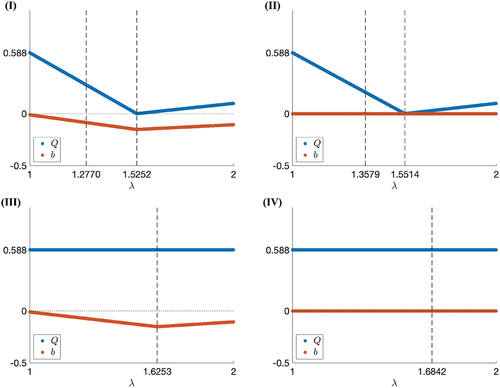
Figure 3. (Colour online) The sine function of the angle $\theta$ between the nematic director in the current and reference configuration for cases (I)–(IV), respectively. For cases (I) and (II), the vertical lines correspond to the predicted longitudinal stretch ratio ${\lambda }_{crt}$ where the director rotates suddenly and the minimum stretch ratio ${\lambda }_{aux}<{\lambda }_{crt}$ where auxeticity is observed. For cases (III) and (IV), the vertical line corresponds to ${\lambda }_{crt}$.

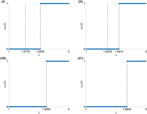
Figure 4. (Colour online) Energy functions for cases (I)–(IV), respectively. For cases (I) and (II), the vertical lines correspond to the predicted longitudinal stretch ratio ${\lambda }_{crt}$ where the director rotates suddenly and the minimum stretch ratio ${\lambda }_{aux}<{\lambda }_{crt}$ where auxeticity is obtained. For cases (III) and (IV), the vertical line corresponds to ${\lambda }_{crt}$.

1. $(Q_0,Q_{crt},Q_1)=(0.5880,0.0010,0.100)$, $(b_0,b_{crt},b_1)=(-0.0102,-0.1518,-0.1056)$, ${\lambda }_{crt}=1.5252$, while the minimum stretch ratio where auxeticity occurs is ${\lambda }_{aux}=1.2770$. Thus, $C_1=-1.1177$, $D_1=1.7057$, $C_2=-1.1177$, $D_2=-0.2227$, $c_1=-0.2696$, $d_1=0.2594$, $c_2=0.0685$, $d_2-0.2562$.

2. $(Q_0,Q_{crt},Q_1)=(0.5880,0.0010,0.1000)$, $b=0$, ${\lambda }_{crt}=1.5514$, and the minimum stretch ratio where auxeticity is observed is ${\lambda }_{aux}=1.3579$. Thus, $C_1=-1.0647$, $D_1=1.6527$, $C_2=-1.0647$, $D_2-0.2358$ and $c_1=c_2=d_1=d_2=0$.

3. $Q=0.5880$, $(b_0,b_{crt},b_1)=(-0.0102,-0.1518,\text{break}-0.1056)$, and ${\lambda }_{crt}=1.6253$. Thus, $C_1=C_2\text{break}=0$, $D_1=D_2=0.5880$, $c_1=-0.2265$, $d_1=0.2163$, $c_2=0.0804$, $d_2=-0.2824$.

4. $Q=0.5880$, $b=0$, and ${\lambda }_{crt}=1.6842$. Thus, $C_1=C_2=0$, $D_1=D_2=0.5880$, $c_1=c_2=d_1\text{break}=d_2=0$.

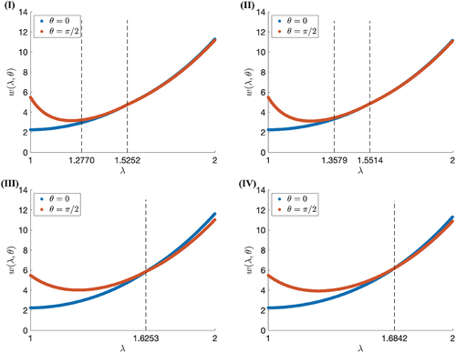
In Figure 4, cases (I) and (II), we note that the plots of the energy function with $\theta =0$ and $\theta =\pi /2$, respectively, appear very close for stretches greater than the critical stretch where the director rotates. However, numerically, and also after a closer inspection of those plots, one can see that the energy with $\theta =\pi /2$, plotted in red, is numerically slightly below that with $\theta =0$, depicted in blue. Before the critical stretch, the energy with $\theta =0$ is below that with $\theta =\pi /2$. In cases (III) and (IV), the difference between the two curves is more pronounced.

Figure 5 shows the corresponding transverse stretch ratios ${\lambda }_2$ and ${\lambda }_3$ as functions of the longitudinal stretch ratio ${\lambda }_1=\lambda$. This figure provides insight into the nature of the auxetic response seen in some LCEs. In case (I), we see how non-constant $Q$ and $b$ lead to a physically realistic deformation. Critically, this case predicts large anisotropy in the transverse stretch ratios ${\lambda }_2$ and ${\lambda }_3$, and also a physically realisable auxetic response. In case (II), where $Q$ varies and $b=0$, a similar behaviour is predicted, but with a less pronounced auxetic response, as the interval between ${\lambda }_{aux}$ and ${\lambda }_{crt}$ is smaller than in case (I). In cases (III) and (IV), although an auxetic reponse is predicted at ${\lambda }_{crt}$, the model shows large discontinuity in ${\lambda }_2$ and ${\lambda }_3$ at ${\lambda }_1={\lambda }_{crt}$, which can be indicative of the fact that the director may rotate slowly rather than suddenly. We can also see that, before ${\lambda }_{crt}$ is reached, in case (III), the non-zero biaxial order parameter allows the evolution of anisotropy in the transverse stretch ratios, while in case (IV), where the uniaxial order parameters is constant, an isotropic deformation in the transverse directions is predicted. Figure 6 displays the associated first Piola-Kirchhoff stresses.

Figure 5. (Colour online) The transverse stretch ratios for cases (I)–(IV), respectively. For cases (I) and (II), the vertical lines correspond to the predicted longitudinal stretch ratio ${\lambda }_{crt}$ where the director rotates suddenly and the minimum stretch ratio ${\lambda }_{aux}<{\lambda }_{crt}$ where auxeticity is obtained. For cases (III) and (IV), the vertical line corresponds to ${\lambda }_{crt}$.

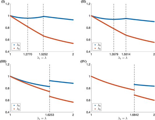
Figure 6. (Colour online) The first Piola-Kirchhoff stresses for cases (I)–(IV), respectively. For cases (I) and (II), the vertical lines correspond to the predicted longitudinal stretch ratio ${\lambda }_{crt}$ where the director rotates suddenly and the minimum stretch ratio ${\lambda }_{aux}<{\lambda }_{crt}$ where auxeticity is obtained. For cases (III) and (IV), the vertical line corresponds to ${\lambda }_{crt}$.

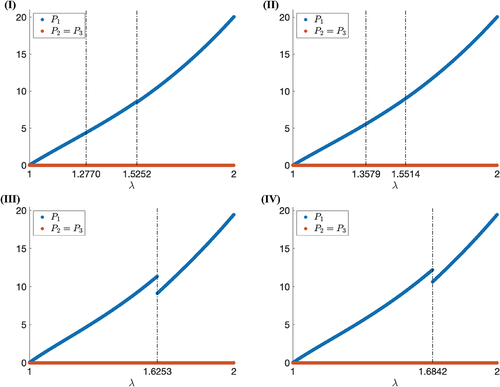
In Figures 2–6, the predicted longitudinal stretch ratio ${\lambda }_{crt}$ where the director rotates suddenly is indicated in each case. For cases (I) and (II), the minimum stretch ratio ${\lambda }_{aux}<{\lambda }_{crt}$ where auxeticity is obtained is also presented.

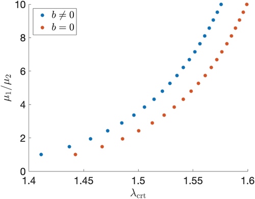
In Figure 7, the critical longitudinal stretch ratios for the director rotation are plotted vs. the parameter ratio ${\mu }_1/{\mu }_2\mathrm{w}\mathrm{h}\mathrm{e}\mathrm{n}n=2(Q_0,Q_{crt},Q_1)=(0.5880,0.0010,$$0.1000)\mathrm{a}\mathrm{n}\mathrm{d}b=0or(b_0,b_{crt},b_1)=(-0.0102,-0.1518,$$-0.1056),$respectively. In both cases, the predicted critical stretch ratio ${\lambda }_{crt}$ increases as ${\mu }_1/{\mu }_2$ increases. In particular, if ${\mu }_2$ is fixed, then ${\lambda }_{crt}$ increases as ${\mu }_1$ increases. Since the shear modulus at infinitesimal strain is equal to $\mu ={\mu }_1+{\mu }_2$, we conclude that ${\lambda }_{crt}$ increases with the linear shear modulus $\mu$, i.e. as the elastic stiffness of the LCE sample increases. This figure further suggests that, for the same parameter ratio ${\mu }_1/{\mu }_2$, if $b=0$, the auxetic response is still captured, but the stretch deformation at which director rotation occurs is slightly delayed compared to when $b\ne 0$.

Figure 7. (Colour online) Predicted longitudinal critical stretch ratio ${\lambda }_{crt}$ for director rotation vs. parameter ratio ${\mu }_1/{\mu }_2$ when $(Q_0,Q_{crt},Q_1)=(0.5880,0.0010,0.1000)$ and $(b_0,b_{crt},b_1)=(-0.0102,-0.1518,-0.1056)$ or $b=0$, respectively.

For the case when the director rotates slowly, in Figure 8, we show the constant uniaxial and biaxial order parameters $Q$ and $b$, respectively, and the stretch ratios ${\lambda }_1=\lambda$ and ${\lambda }_2={\lambda }_3=1/\sqrt{\lambda }$. The constant anisotropy parameter given by Equation (28)(28) $a=\frac{1+2Q}{1-Q}$(28) when $Q=0.5880$ is $a=5.2816$.

Figure 8. (Colour online) The two vertical lines correspond to the lower and upper bounds $[{\lambda }_{\ast },{\lambda }^{\ast }]=[1.5900,1.8548]$ on the extension ratio $\lambda$, between which shear striping occurs.

Figure 9 depicts the strain-energy function $w(\lambda ,\epsilon ,\theta )$ defined by Equation (38)(38) $w(\lambda ,\epsilon ,\theta )=W^{(lce)}({\lambda }_1,{\lambda }_2,{\lambda }_3,Q,b,\theta ),$(38) , for $(\epsilon ,\theta )=(0,0)$, $(\epsilon ,\theta )=({\epsilon }_0,{\theta }_0)$, and $(\epsilon ,\theta )=(0,\pi /2)$. The predicted longitudinal stretch ratio interval where shear striping occurs is $[{\lambda }_{\ast },{\lambda }^{\ast }]=[1.5900,1.8548]$. In Figure 10, the sine of the director angle ${\theta }_0$ and the shear parameter ${\epsilon }_0$ are illustrated for various parameter ratios ${\mu }^{(1)}/{\mu }^{(2)}$. 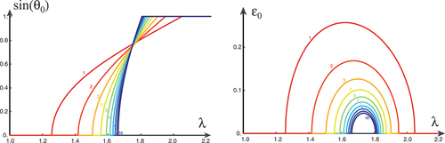These results are in qualitative agreement with those shown in [15,33]. Similar theoretical results can be found, for example, in Refs [21,23,24] (see also [34, Chapter 6]).

Figure 9. (Colour online) The energy function when the director rotates slowly. The two vertical lines correspond to the lower and upper bounds $[{\lambda }_{\ast },{\lambda }^{\ast }]=[1.5900,1.8548]$ on the extension ratio $\lambda$, between which the second solution, with $(\epsilon ,\theta )=({\epsilon }_0,{\theta }_0)$, minimises the energy.

Figure 10. (Colour online) The sine of the director angle ${\theta }_0$ and the shear parameter ${\epsilon }_0$ during stripe formation in the case when the director rotates slowly for values of ${\mu }_1/{\mu }_2$ from 1 to 10 (as labelled).

4. Conclusion

LCE stretching ultimately causes a reorientation of the nematic director which tends to become parallel to the applied force. Sometimes a change in order also occurs. This correlation between macroscopic deformation and molecular architecture causes a variety of mechanical instabilities not observed in conventional rubber-like solids.

For example, experimental evidence demonstrates that, for LCEs with planar mesogen alignment, when a uniaxial tensile force is imposed perpendicular to the nematic director, the director rotates either slowly giving rise to a shear stripe pattern or almost suddenly causing auxeticity at a characteristic large strain. Experimentally, for auxetic LCEs, biaxiality has also been found to emerge.

The present theoretical study proposes a general mathematical model capable of predicting either the classical shear-striping instability or the auxetic response observed in various LCEs. From the modelling point of view, these two phenomena are captured by letting the uniaxial scalar order parameter decrease continuously to a sufficiently low value then increase again in the case of auxetic LCEs, and by maintaining it constant for LCEs exhibiting shear stripes. The theoretical model further suggests that biaxiality also plays a role in enhancing the auxetic reponse. These results may shed some light on the role of nematic order in the observed mechanical behaviours.

Further experimental investigation where nematic parameters must be varied systematically is required to fully understand the auxetic phenomenon and will be a subject for our future study.

Disclosure statement

No potential conflict of interest was reported by the authors.

Data availability statement

All supporting data for this research are included in the paper.

Additional information

Funding

We are grateful for the support by the Engineering and Physical Sciences Research Council of Great Britain under research grants EP/R020205/1 to AG, EP/S028870/1 to LAM and EP/M009521/1 to HFG. DM thanks the Leverhulme Trust for an Early Career Fellowship.

References

- Mistry D, Morgan PB, Clamp JH, et al. New insights into the nature of semi-soft elasticity and “mechanical-Fréedericksz transitions” in liquid crystal elastomers. Soft Matter. 2018;14(8):1301–1310.
- Mistry D, Connell SD, Mickthwaite SL, et al. Coincident molecular auxeticity and negative order parameter in a liquid crystal elastomer. Nat Commun. 2018;9(1):5095.
- Mistry D, Gleeson HF. Mechanical deformations of a liquid crystal elastomer at director angles between 0° and 90°: deducing an empirical model encompassing anisotropic nonlinearity. J Polym Sci. 2019;57:1367–1377. DOI:10.1002/polb.24879
- Mistry D, Nikkhou M, Raistrick T, et al. Isotropic liquid crystal elastomers as exceptional photoelastic strain sensors. Macromolecules. 2020;53(10):3709–3718.
- Raistrick T, Zhang Z, Mistry D, et al. Understanding the physics of the auxetic response in a liquid crystal elastomer. Phys Rev Res. 2021;3(2):023191.
- Raistrick T, Reynolds M, Gleeson HF, et al. Influence of liquid crystallinity and mechanical deformation on the molecular relaxations of an auxetic liquid crystal elastomer. Molecules. 2021;26(23):7313.
- Finkelmann H, Kundler I, Terentjev EM, et al. Critical stripe-domain instability of nematic elastomers. J Phys II. 1997;7(8):1059–1069.
- Kundler I, Finkelmann H. Strain-induced director reorientation in nematic liquid single crystal elastomers. Macromol Rapid Commun. 1995;16(9):679–686.
- Kundler I, Finkelmann H. Director reorientation via stripe-domains in nematic elastomers: influence of cross-link density, anisotropy of the network and smectic clusters. Macromol Chem Phys. 1998;199(4):677–686.
- Petelin A, Čopič M. Observation of a soft mode of elastic instability in liquid crystal elastomers. Phys Rev Lett. 2009;103(7):077801.
- Petelin A, Čopič M. Strain dependence of the nematic fluctuation relaxation in liquid-crystal elastomerss. Phys Rev E. 2010;82(1):011703.
- Talroze RV, Zubarev ER, Kuptsov SA, et al. Liquid crystal acrylate-based networks: polymer backbone–LC order interaction. React Funct Polym. 1999;41(1–3):1–11.
- Zubarev ER, Kuptsov SA, Yuranova TI, et al. Monodomain liquid crystalline networks: reorientation mechanism from uniform to stripe domains. Liq Cryst. 1999;26(10):1531–1540.
- Mitchell GR, Davis FJ, Guo W. Strain-induced transition in liquid-crystal elastomers. Phys Rev Lett. 1993;71(18):2947.
- Warner M, Terentjev EM. Liquid Crystal Elastomers. Oxford, UK: Oxford University Press; 2007.
- Conti S, DeSimone A, Dolzmann G. Soft elastic response of stretched sheets of nematic elastomers: a numerical study. J Mech Phys Solids. 2002;50(7):1431–1451.
- DeSimone A, Dolzmann G. Material instabilities in nematic elastomers. Physica D. 2000;136(1–2):175–191.
- DeSimone A, Teresi L. Elastic energies for nematic elastomers. Eur Phys J E. 2009;29(2):191–204.
- Fried E, Sellers S. Free-energy density functions for nematic elastomers. J Mech Phys Solids. 2004;52(7):1671–1689.
- Fried E, Sellers S. Orientational order and finite strain in nematic elastomers. J Chem Phys. 2005;123(4):043521.
- Fried E, Sellers S. Soft elasticity is not necessary for striping in nematic elastomers. J Appl Phys. 2006;100(4):043521.
- Goriely A, Mihai LA. Liquid crystal elastomers wrinkling. Nonlinearity. 2021;34(8):5599–5629.
- Mihai LA, Goriely A. Likely striping in stochastic nematic elastomers. Math Mech Solids. 2020;25(10):1851–1872.
- Mihai LA, Goriely A. Instabilities in liquid crystal elastomers. MRS Bull. 2021;46(9):784–794.
- Mihai LA, Mistry D, Raistrick T, et al. A mathematical model for the auxetic response of liquid crystal elastomers. Philos Trans R Soc A. 2022;380(2234):20210326.
- Ogden RW. Large deformation isotropic elasticity - on the correlation of theory and experiment for incompressible rubberlike solids. Proc R Soc Lond A. 1972;326:565–584.
- Ogden RW. Non-linear elastic deformations. New York (NY): Dover; 1997.
- Mistry D. The richness of liquid crystal elastomer mechanics keeps growing. Liq Cryst Today. 2021;30(4):59–66.
- Finkelmann H, Greve A, Warner M. The elastic anisotropy of nematic elastomers. Eur Phys J E. 2001;5(3):281–293.
- de Gennes PG, Prost J. The physics of liquid crystals. Oxford: Clarendon Press; 1993.
- Urayama K, Mashita R, Kobayashi I, et al. Stretching-induced director rotation in thin films of liquid crystal elastomers with homeotropic alignment. Macromolecules. 2007;40(21):7665–7670.
- Higaki H, Takigawa T, Urayama K. Nonuniform and uniform deformations of stretched nematic elastomers. Macromolecules. 2013;46(13):5223–5231.
- Verwey GC, Warner M, Terentjev EM. Elastic instability and stripe domains in liquid crystalline elastomers. J Phys. 1996;6(9):1273–1290.
- Mihai LA. Stochastic elasticity: a nondeterministic approach to the nonlinear field theory. Switzerland: Springer; 2022. doi:10.1007/978-3-031-06692-4.