A free discontinuity model for smectic thin films

ABSTRACT

We attempt to describe surface defects in smectic A thin films by formulating a free discontinuity problem – that is, a variational problem in which the order parameter is allowed to have jump discontinuities on some (unknown) set. The free energy functional contains an interfacial energy, which penalises dislocations of the smectic layers at the jump. We discuss mathematical issues related to the existence of minimisers and provide examples of minimisers in some simplified settings.

Graphical abstract

KEYWORDS:

• Smectic liquid crystals
• surface defects
• special functions of bounded variation
• BV ellipticity

1. Introduction

In this paper, we report on an attempt to formulate a mathematical model, capable of rigorous mathematical analysis, to describe aspects of the interesting experiments on smectic A thin films of the group of E. Lacaze [1–5]. In these experiments, thin films of 8CB liquid crystal are deposited on various substrates, for example, $\mathrm{M}\mathrm{o}{\mathrm{S}}_2$, mica and rubbed PVA. Depending on the thickness of the films and on the nature of the substrate different configurations of the smectic layers are observed [6]. The main features are illustrated in Figures 1 and 2. Viewed from above (Figure 1) families of parallel ‘oily streaks’ are observed, each of which consists of a flattened hemi cylinder of smectic layers (Figure 2). The representation in Figure 2 of the configuration of layers in an oily streak on a rubbed PVA substrate is not a direct observation, but is deduced from X-ray diffraction and ellipsometry; indeed, recently, some slight modifications to the likely configuration have been suggested by Jeridi et al. [7].

Figure 1. AFM image of families of oily streaks of 8CB on $\mathrm{M}\mathrm{o}{\mathrm{S}}_2$ substrate. Reprinted with permission from [1] (copyright 2014, American Physical Society).

Figure 2. (Colour online) Experimental representation of cross-sectional layer configuration in an oily streak of 8CB on PVA substrate. Reproduced from [5] with permission from the Royal Society of Chemistry.

The observed layer configurations are a consequence of the antagonistic boundary conditions, homeotropic on the upper surface in contact with air, and unidirectional planar anchoring on the bottom surface parallel to the substrate. Because for smectic A the director $\mathbf{n}$ is perpendicular to the layers, this means that the layers prefer energetically to be tangent to the upper free surface and perpendicular to the substrate.

A feature of the observed layer configurations is the presence of surface (wall) defects across which the layer normal, and thus $\mathbf{n}$, jumps. This suggests that a good mathematical framework to handle this problem is the free discontinuity setting originated by De Giorgi & Ambrosio [8] for image segmentation and subsequently used by Francfort & Marigo for Griffith fracture models [9]. The relevance of such a setting for liquid crystal problems was proposed in [10]. The free discontinuity formulation uses a free energy in which there is a competition between bulk (volumetric) energy and interfacial energy corresponding to unknown surfaces of discontinuity. In the case of fracture mechanics, the bulk energy is the elastic energy, and the interfacial energy is located on the unknown crack surfaces. For smectic A thin films, we will take the bulk energy to be the elastic (Oseen-Frank) energy, and the discontinuity surfaces will correspond to walls across which $\mathbf{n}$ jumps.

The thin-film experiments described above would best be treated as a free boundary problem for a given volume of liquid crystal deposited on the substrate, with the aim of predicting the possible 3D configurations of oily streaks as well as their internal structure. A key prediction of such a model would be the width of the oily streaks. However, we are not currently able to give conditions under which the minimum of the corresponding energy is attained, and if so by what configurations of layers.

Instead, we will work on a fixed domain $\mathrm{\Omega }\subset {\mathbb{R}}^2$, to be thought of as the cross-section of an oily streak, and seek to predict the corresponding configurations of layers given suitable boundary conditions.

2. The model

2.1. The elastic energy

We use as a basic variable the director $\mathbf{n}$, $|\mathbf{n}|=1$, which for smectic A is parallel to the layer normal $\mathbf{m}$, so that $\mathbf{n}\otimes \mathbf{n}=\mathbf{m}\otimes \mathbf{m}$. The three-dimensional Oseen-Frank energy density

$\begin{array}{rl}& W(\mathbf{n},\mathrm{\nabla }\mathbf{n})=\frac{1}{2}\left(K_1{(\mathrm{d}\mathrm{i}\mathrm{v}\mathbf{n})}^2\right.+K_2(\mathbf{n}\cdot \mathrm{c}\mathrm{u}\mathrm{r}\mathrm{l}\mathbf{n}{)}^2+K_3{\left|\mathbf{n}\wedge \mathrm{c}\mathrm{u}\mathrm{r}\mathrm{l}\mathbf{n}\right|}^2\\ & +(K_2+K_4)\left.(\mathrm{t}\mathrm{r}{(\mathrm{\nabla }\mathbf{n})}^2-{(\mathrm{d}\mathrm{i}\mathrm{v}\mathbf{n})}^2)\right),(1)\end{array}$

with Frank constants $K_i$, is invariant to changing the sign of $\mathbf{n}$, and thus can be expressed in terms of $\mathbf{M}:=\mathbf{n}\otimes \mathbf{n}$ and $\mathrm{\nabla }\mathbf{M}$. For example, we have that

(2) $\begin{array}{rl}& |\mathbf{n}\wedge \mathrm{c}\mathrm{u}\mathrm{r}\mathrm{l}\mathbf{n}{|}^2=|(\mathbf{n}\cdot \mathrm{\nabla })\mathbf{n}{|}^2\\ & =\frac{1}{2}{M}_{rs}{M}_{ij,r}{M}_{ij,s},\end{array}$(2)

where $M_{ij}=n_i{n}_j$ and we have used $2n_i{n}_{i,j}=(|\mathbf{n}{|}^2{)}_{,j}=0$. We make the assumption of constant layer thickness (or locally parallel layers), which for sufficiently smooth $\mathbf{m}$ is equivalent to the condition $\mathrm{c}\mathrm{u}\mathrm{r}\mathrm{l}\mathbf{m}=0$, and thus (assuming $\mathbf{n}$ sufficiently smooth so that we can take $\mathbf{n}=\mathbf{m}$) to the condition $\mathrm{c}\mathrm{u}\mathrm{r}\mathrm{l}\mathbf{n}=0$.

We assume two-dimensional symmetry for $\mathbf{n}$, so that for $\mathbf{x}=(x_1,x_2)\in \mathrm{\Omega }$

(3) $\mathbf{n}(\mathbf{x})=(\mathbf{n}(x_1,x_2),0)$(3)

with $\mathbf{n}(x_1,x_2)\in {\mathbb{S}}^1$, where ${\mathbb{S}}^1$ is the unit circle. For such two-dimensional director fields, an explicit computation shows that the term $\mathrm{t}\mathrm{r}(\mathrm{\nabla }\mathbf{n}{)}^2-(\mathrm{d}\mathrm{i}\mathrm{v}\mathbf{n}{)}^2$ is identically equal to zero so that, taking into account also the constraint $\mathrm{c}\mathrm{u}\mathrm{r}\mathrm{l}\mathbf{n}=0$, the Oseen-Frank energy (1) reduces to

(4) $W(\mathbf{n},\mathrm{\nabla }\mathbf{n})=\frac{1}{2}{K}_1|\mathrm{\nabla }\mathbf{n}{|}^2,$(4)

where we assume that $K_1>0$. This is the original model for smectics proposed by Oseen [11]. It can be viewed as a special case $\mathbf{m}=\mathbf{n}$ of the model of [12]. There are various other models for smectics allowing variable layer thickness ([13–16]), that typically introduce the molecular number density $\rho =\rho (\mathbf{x})$ or fluctuations about it as a new macroscopic variable, with the smectic layers being seen as density waves. These models can describe dislocations in smectic layers, for example, although it is unclear how to understand the macroscopic variable $\rho$ varying over a molecular length-scale.

To allow for nonorientable configurations, we reformulate the problem in terms of the two-dimensional $\mathbf{Q}$-tensor

(5) $\mathbf{Q}:=\frac{1}{\sqrt{2}}\left(\mathbf{n}\otimes \mathbf{n}-\frac{\mathbf{I}}{2}\right)$(5)

where $\mathbf{I}$ is the $2\times 2$ identity matrix. The constant $1/\sqrt{2}$ is a normalisation factor, which plays no essential role in our analysis. At each point $\mathbf{x}\in \mathrm{\Omega }$, $\mathbf{Q}(\mathbf{x})$ is a symmetric trace-free $2\times 2$ matrix, which belongs to the set

(6) $\mathcal{N}:=\left\{\frac{1}{\sqrt{2}}\left(\mathbf{n}\otimes \mathbf{n}-\frac{\mathbf{I}}{\mathbf{2}}\right):\mathbf{n}\in {\mathbb{S}}^1\right\}.$(6)

If $\mathbf{n}:\mathrm{\Omega }\to {\mathbb{S}}^1$ is a smooth vector field and $\mathbf{Q}$ is defined as in (5), an explicit computation shows that ${\left|\mathrm{\nabla }\mathbf{n}\right|}^2={\left|\mathrm{\nabla }\mathbf{Q}\right|}^2:=Q_{ij,k}{Q}_{ij,k}$, expressing the elastic energy (4) in terms of $\mathbf{Q}$.

We also need to express the constraint $\mathrm{c}\mathrm{u}\mathrm{r}\mathrm{l}\mathbf{n}=0$ in terms of $\mathbf{Q}$. We define

$\mathbf{A}(\mathbf{Q})(\mathrm{\nabla }\mathbf{Q},\mathrm{\nabla }\mathbf{Q}):=\left(\sqrt{2}{Q}_{hk}+\frac{1}{2}{\delta }_{hk}\right)Q_{ij,h}{Q}_{ij,k}.$

This is a quadratic form in $\mathrm{\nabla }\mathbf{Q}$, reminiscent of the cubic term in the Landau-de Gennes elastic energy (see, e.g. [[17], Section 4]). Thanks to (2), (5), we find that

$\begin{array}{c}\mathbf{A}(\mathbf{Q})(\mathrm{\nabla }\mathbf{Q},\mathrm{\nabla }\mathbf{Q})=|\mathbf{n}\wedge \mathrm{c}\mathrm{u}\mathrm{r}\mathrm{l}\mathbf{n}{|}^2,\end{array}$

and since ${\left|\mathrm{c}\mathrm{u}\mathrm{r}\mathrm{l}\mathbf{n}\right|}^2={\left|\mathbf{n}\wedge \mathrm{c}\mathrm{u}\mathrm{r}\mathrm{l}\mathbf{n}\right|}^2+(\mathbf{n}\cdot \mathrm{c}\mathrm{u}\mathrm{r}\mathrm{l}\mathbf{n}{)}^2$, and keeping in mind that a two-dimensional vector field is orthogonal to its curl, we obtain $\mathbf{A}(\mathbf{Q})(\mathrm{\nabla }\mathbf{Q},\mathrm{\nabla }\mathbf{Q})={\left|\mathrm{c}\mathrm{u}\mathrm{r}\mathrm{l}\mathbf{n}\right|}^2$. Therefore, we impose the constraint

(7) $\mathbf{A}(\mathbf{Q})(\mathrm{\nabla }\mathbf{Q},\mathrm{\nabla }\mathbf{Q})=0,$(7)

which expresses the constant layer thickness in terms of $\mathbf{Q}$.

2.2. The function space

In order to specify in precise mathematical terms any energy minimisation problem, it is necessary to say in which function space the minimum is sought. The function space describes the allowed singularities of the unknown function or map and is part of the model. Making the function space larger, so that worse singularities are allowed, may lead to different minimisers (this is known as the Lavrentiev phenomenon, see [[17], Section 3]). The main function space used for free discontinuity problems, and developed by De Giorgi and Ambrosio [8], is the space SBV of special functions of bounded variation. In fact, in this work, we will consider a slight variant of the space $\mathrm{S}\mathrm{B}\mathrm{V}$, i.e. the space $\mathrm{S}\mathrm{B}{\mathrm{V}}^2$. Let $\mathrm{\Omega }$ be an open, bounded planar region. In technical terms, a map $\mathbf{u}:\mathrm{\Omega }\to {\mathbb{R}}^m$ belongs to $\mathrm{S}\mathrm{B}{\mathrm{V}}^2(\mathrm{\Omega },{\mathbb{R}}^m)$ if its distributional derivative $\mathrm{D}\mathbf{u}$ is a finite measure with no Cantor part, and whose absolutely continuous part $\mathrm{\nabla }\mathbf{u}$ is square integrable (see, e.g. [8,18] for more details). For the purposes of this paper, the key points of the definition and theory are the following:

1. for any $\mathbf{u}\in \mathrm{S}\mathrm{B}{\mathrm{V}}^2(\mathrm{\Omega },{\mathbb{R}}^m)$ there is a one-dimensional jump set ${\mathrm{S}}_{\mathbf{u}}$ consisting of the points $\mathbf{x}\in \mathrm{\Omega }$ at which $\mathbf{u}$ has a jump discontinuity,

2. for (almost) any point $\mathbf{x}\in {\mathrm{S}}_{\mathbf{u}}$ there is a well-defined unit normal $\mathit{\nu }(\mathbf{x})={\mathit{\nu }}_{\mathbf{u}}(\mathbf{x})$ to ${\mathrm{S}}_{\mathbf{u}}$ and well-defined limits ${\mathbf{u}}^{+}(\mathbf{x}),{\mathbf{u}}^{-}(\mathbf{x})$ from either side of ${\mathrm{S}}_{\mathbf{u}}$. There may be an exceptional set of points $\mathbf{x}\in {\mathrm{S}}_{\mathbf{u}}$ at which $\mathit{\nu }(\mathbf{x})$, ${\mathbf{u}}^{+}(\mathbf{x})$ or ${\mathbf{u}}^{-}(\mathbf{x})$ are not defined, but this must be a set of zero length;

3. the gradient $\mathrm{\nabla }\mathbf{u}$ is defined in $\mathrm{\Omega }\mathrm{\setminus }{\mathrm{S}}_{\mathbf{u}}$ and ${\int }_{\mathrm{\Omega }}|\mathrm{\nabla }\mathbf{u}(\mathbf{x}){|}^2\mathrm{d}\mathbf{x}<+\mathrm{\infty }$.

The space $\mathrm{S}\mathrm{B}{\mathrm{V}}^2(\mathrm{\Omega },{\mathbb{R}}^{2\times 2})$, whose elements are $2\times 2$ matrix fields on $\mathrm{\Omega }$ in the class $\mathrm{S}\mathrm{B}{\mathrm{V}}^2$, is defined analogously by identifying ${\mathbb{R}}^{2\times 2}$ with ${\mathbb{R}}^4$.

As we are considering a free discontinuity problem, the map $\mathbf{Q}$ is allowed to have jump discontinuities on a one-dimensional set ${\mathrm{S}}_{\mathbf{Q}}$, and the condition (7) loses its meaning at points of ${\mathrm{S}}_{\mathbf{Q}}$. Therefore, the constraint (7) is only enforced in the complement $\mathrm{\Omega }\mathrm{\setminus }{\mathrm{S}}_{\mathbf{Q}}$. In technical terms, (7) only involves the absolutely continuous part $\mathrm{\nabla }\mathbf{Q}$ of the distributional derivative of $\mathbf{Q}$.

2.3. The jump energy

Let

(8) $\mathrm{S}\mathrm{B}{\mathrm{V}}^2(\mathrm{\Omega },\mathcal{N}):=\left\{\mathbf{Q}\in \mathrm{S}\mathrm{B}{\mathrm{V}}^2(\mathrm{\Omega },{\mathbb{R}}^{2\times 2}),\mathbf{Q}(x)\in \mathcal{N}\mathrm{f}\mathrm{o}\mathrm{r}x\in \mathrm{\Omega }\right\}$(8)

be the set of $\mathcal{N}$-valued $\mathbf{Q}$-tensors in the class $\mathrm{S}\mathrm{B}{\mathrm{V}}^2$. For $\mathbf{Q}\in \mathrm{S}\mathrm{B}{\mathrm{V}}^2(\mathrm{\Omega },\mathcal{N})$, we consider the jump energy

(9) ${\int }_{{\mathrm{S}}_{\mathbf{Q}}}\phi ({\mathbf{Q}}^{+},{\mathbf{Q}}^{-},\mathit{\nu })\mathrm{d}{\mathcal{H}}^1$(9)

where the integral is taken over the (one-dimensional) jump set ${\mathrm{S}}_{\mathbf{Q}}$, with respect to the length measure $\mathrm{d}{\mathcal{H}}^1$, and $\phi :\mathcal{N}\times \mathcal{N}\times {\mathbb{S}}^1\to \mathbb{R}$ is a continuous function. We want to choose the jump energy density $\phi$ so that (9) is a good model for the energy of a defect wall. Natural conditions on $\phi$ are:

(C1) $\phi ({\mathbf{Q}}^{+},{\mathbf{Q}}^{-},\nu )=0$ if ${\mathbf{Q}}^{+}={\mathbf{Q}}^{-}$;

(C2) invariance with respect to the orientation of the jump set, that is

$\phi ({\mathbf{Q}}^{-},{\mathbf{Q}}^{+},-\mathit{\nu })=\phi ({\mathbf{Q}}^{+},{\mathbf{Q}}^{-},\mathit{\nu })$

for any ${\mathbf{Q}}^{+}\in \mathcal{N}$, ${\mathbf{Q}}^{-}\in \mathcal{N}$, $\mathit{\nu }\in {\mathbb{S}}^1$;

(C3) frame-indifference, that is

$\phi (\mathbf{R}{\mathbf{Q}}^{+}{\mathbf{R}}^T,\mathbf{R}{\mathbf{Q}}^{-}{\mathbf{R}}^T,\mathbf{R}\mathit{\nu })=\phi ({\mathbf{Q}}^{+},{\mathbf{Q}}^{-},\mathit{\nu })$

for all ${\mathbf{Q}}^{+}\in \mathcal{N}$, ${\mathbf{Q}}^{-}\in \mathcal{N}$, $\mathit{\nu }\in {\mathbb{S}}^1$ and all orthogonal matrices $\mathbf{R}\in \mathrm{O}(2)$.

Another condition we impose is that $\phi$ should penalise dislocations of the smectic layers. Generically, it may not be possible to define the smectic layers consistently across the jump set, because there may be dislocations. A geometric condition for the layers to match at the jump set is that, at each jump point, the normal to the jump set $\mathit{\nu }$ bisects any of the angles between the smectic layers. For smectic A liquid crystals, the layers are orthogonal to the molecular directors ${\mathbf{n}}^{+}$, ${\mathbf{n}}^{-}$ on either side of the jump, so bisecting any of the angles between the layers is equivalent to bisecting any of the angles between ${\mathbf{n}}^{+}$ and ${\mathbf{n}}^{-}$. This can be written as

(10) $({\mathbf{n}}^{+}\cdot \mathit{\nu }{)}^2=({\mathbf{n}}^{-}\cdot \mathit{\nu }{)}^2$(10)

or equivalently, in terms of the $\mathbf{Q}$-tensor, as

(11) ${\mathbf{Q}}^{+}\mathit{\nu }\cdot \mathit{\nu }={\mathbf{Q}}^{-}\mathit{\nu }\cdot \mathit{\nu }.$(11)

In order to penalise dislocations, we therefore impose the following condition on $\phi$:

(C4) for given ${\mathbf{Q}}^{+},{\mathbf{Q}}^{-}\in \mathcal{N}$, the function $\mathit{\nu }\in {\mathbb{S}}^1\mapsto \phi ({\mathbf{Q}}^{+},{\mathbf{Q}}^{-},\mathit{\nu })$ is minimised for a $\mathit{\nu }$ satisfying (11).

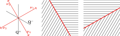
Given distinct ${\mathbf{Q}}^{+}$ and ${\mathbf{Q}}^{-}$, there are four such $\mathit{\nu }$ that bisect the angles between the corresponding directors ${\mathbf{n}}^{+}$, ${\mathbf{n}}^{-}$; we label them as ${\mathit{\nu }}_1$, ${\mathit{\nu }}_2$, ${\mathit{\nu }}_3=-{\mathit{\nu }}_1$ and ${\mathit{\nu }}_4=-{\mathit{\nu }}_2$, as in Figure 3. By taking $\mathbf{R}=-\mathbf{I}$ in condition (C3), we obtain that $\phi ({\mathbf{Q}}^{+},{\mathbf{Q}}^{-},{\mathit{\nu }}_1)=\phi ({\mathbf{Q}}^{+},{\mathbf{Q}}^{-},{\mathit{\nu }}_3)$ and $\phi ({\mathbf{Q}}^{+},{\mathbf{Q}}^{-},{\mathit{\nu }}_2)=\phi ({\mathbf{Q}}^{+},{\mathbf{Q}}^{-},{\mathit{\nu }}_4)$. However, we must account for the possibility that, in general, $\phi ({\mathbf{Q}}^{+},{\mathbf{Q}}^{-},{\mathit{\nu }}_1)\ne \phi ({\mathbf{Q}}^{+},{\mathbf{Q}}^{-},{\mathit{\nu }}_2)$. Indeed, configurations whose jump sets are oriented according to the unit normal ${\mathit{\nu }}_1$ or ${\mathit{\nu }}_2$ have (generically) different geometric properties, because ${\mathbf{Q}}^{+}{\mathit{\nu }}_1\cdot {\mathit{\nu }}_1\ne {\mathbf{Q}}^{+}{\mathit{\nu }}_2\cdot {\mathit{\nu }}_2$ unless the directors ${\mathbf{n}}^{+}$, ${\mathbf{n}}^{-}$ corresponding to ${\mathbf{Q}}^{+}$, ${\mathbf{Q}}^{-}$ are orthogonal to each other. The condition (C4) is compatible with an energy density that, as a function of $\mathit{\nu }$, has two global minima at ${\mathit{\nu }}_1$, ${\mathit{\nu }}_3$ (or, respectively, at ${\mathit{\nu }}_2$, ${\mathit{\nu }}_4$) and, say, two local minima at ${\mathit{\nu }}_2$, ${\mathit{\nu }}_4$ (respectively, at ${\mathit{\nu }}_1$, ${\mathit{\nu }}_3$), at a possibly higher energy value.

Figure 3. (Colour online) Left: given $\mathbf{Q}$⁺ and $\mathbf{Q}$^–, there are four unit vectors ${\mathit{\nu }}_1$, ${\mathit{\nu }}_2$, ${\mathit{\nu }}_3$, ${\mathit{\nu }}_4$ that satisfy (10). The $\mathbf{Q}$-tensors $\mathbf{Q}$⁺ and $\mathbf{Q}$^– are represented by (arrowless black) straight lines, oriented parallel to the molecular directors $\mathbf{n}$⁺, $\mathbf{n}$^– corresponding to $\mathbf{Q}$⁺, $\mathbf{Q}$^– respectively. Here $\mathbf{Q}$⁺ and $\mathbf{n}$⁺ (respectively, $\mathbf{Q}$^– and $\mathbf{n}$^–) are related to each other by (5). Centre and right: two piecewise constant configurations that satisfy (10). The black lines represent the smectic layers, which are orthogonal to the molecular director, and the thick red line represents the jump.

A singular jump energy satisfying all the conditions (C1)–(C4) is given by

(12) ${\zeta }_{\alpha }({\mathbf{Q}}^{+},{\mathbf{Q}}^{-},\mathit{\nu }):=\left\{\begin{array}{cc}{\left|{\mathbf{Q}}^{+}-{\mathbf{Q}}^{-}\right|}^{\alpha }& \mathrm{i}\mathrm{f}{\mathbf{Q}}^{+}\mathit{\nu }\cdot \mathit{\nu }={\mathbf{Q}}^{-}\mathit{\nu }\cdot \mathit{\nu }\\ +\mathrm{\infty }& \mathrm{o}\mathrm{t}\mathrm{h}\mathrm{e}\mathrm{r}\mathrm{w}\mathrm{i}\mathrm{s}\mathrm{e},\end{array}\right.$(12)

where $\alpha$ is a parameter such that $0<\alpha <1$. Choosing $\alpha >0$ guarantees that the condition (C1) is satisfied. On the other hand, taking $\alpha <1$ is required for reasons of mathematical consistency; had we taken $\alpha \ge 1$, then there would be no guarantee that a minimiser for the energy functional exists in the space $\mathrm{S}\mathrm{B}{\mathrm{V}}^2(\mathrm{\Omega },\mathcal{N})$. 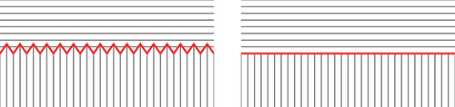(We do not discuss this issue in detail and refer to e.g [18], Sections 4.1–2.) However, even if the parameter $\alpha$ is chosen carefully, the functional associated with (12) suffers from a mathematical pathology, which is illustrated in Figure 4: there exist sequences ${\mathbf{Q}}_j\in \mathrm{S}\mathrm{B}\mathrm{V}(\mathrm{\Omega },\mathcal{N})$ that converge to a limit map $\mathbf{Q}\in \mathrm{S}\mathrm{B}\mathrm{V}(\mathrm{\Omega },\mathcal{N})$ in a suitable sense, yet the energy of $\mathbf{Q}$ is strictly larger than the limit, as $j\to +\mathrm{\infty }$, of the energy of ${\mathbf{Q}}_j$. This behaviour, known as lack of lower semicontinuity, is particularly evident in Figure 4, because the energy of the limit configuration is infinite. However, even if we considered a modified energy density that takes only finite values, this pathological behaviour could persist. The main issue is that the energy density ${\zeta }_{\alpha }$ is not BV-elliptic. BV-ellipticity, which was introduced by Ambrosio and Braides [19], is a necessary condition for the lower semicontinuity of the energy functional, and is an important assumption to ensure the existence of minimisers of free discontinuity problems [19,20].

Figure 4. (Colour online) A mathematical pathology associated with the energy density ${\zeta }_{\alpha }$, given by (12). The black lines represent the smectic layers, while the thick red line represents the jump set. On the left, a piecewise constant configuration in a rectangle, with a zig-zag interface and zig-zag angles of $45$ degrees; on the right, a piecewise constant configuration with a horizontal jump set. If we choose the energy density as in (12), the energy of the configuration on the left is $\sqrt{2}b\mu$, where $b$ is the length of the bottom base of the rectangle, irrespective of the spacing of the zig-zag. As the latter tends to zero, the configuration on the left converges (in a suitable sense) to that on the right, which costs an infinite energy.

We briefly explain the notion of BV-ellipticity. Let ${\mathbf{Q}}^{+}\in \mathcal{N}$, ${\mathbf{Q}}^{-}\in \mathcal{N}$, $\mathit{\nu }\in {\mathbb{S}}^1$ be given. Let $C$ be a (closed) unit square, centred at the origin, whose sides are parallel to $\mathit{\nu }$ and to ${\mathit{\nu }}^{\mathrm{\perp }}:=({\nu }_2,-{\nu }_1)$ (see Figure 5). Let $C{ }^{\mathrm{\prime }}$ be a slightly larger such square, such that $C$ is contained in the interior of $C{ }^{\mathrm{\prime }}$. We consider a piecewise constant map ${\mathbf{Q}}^{\ast }\in \mathrm{S}\mathrm{B}\mathrm{V}(C{ }^{\mathrm{\prime }},\mathcal{N})$, defined as

Figure 5. (Colour online) The domain and boundary conditions in the definition of BV-ellipticity (Definition 2.1). The domain $C$ is a unit square, rotated in such a way that the sides are parallel to $\mathit{\nu }$, ${\mathit{\nu }}^{\mathrm{\perp }}$. The ‘boundary conditions’, defined in a collar of $\mathrm{\partial }C$, are piecewise constant and are defined by $\mathbf{Q}$⁺ and $\mathbf{Q}$^–. The admissible configurations $\mathbf{P}$ are piecewise constant inside $C$ (and are allowed to take finitely many values only).

(13) ${\mathbf{Q}}^{\ast }(\mathrm{x}):=\left\{\begin{array}{c}{\mathbf{Q}}^{+}\mathrm{i}\mathrm{f}\mathbf{x}\cdot \mathit{\nu }>0\\ {\mathbf{Q}}^{-}\mathrm{i}\mathrm{f}\mathbf{x}\cdot \mathit{\nu }<\hspace{0.17em}0\end{array}\right.$(13)

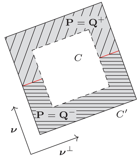
The map ${\mathbf{Q}}^{\ast }$ jumps along a straight line orthogonal to $\mathit{\nu }$. The notion of BV-ellipticity is defined in terms of a suitable minimisation problem. Let $\mathcal{C}[{\mathbf{Q}}^{+},{\mathbf{Q}}^{-},\mathit{\nu }]$ be the class of all maps $\mathbf{P}\in \mathrm{S}\mathrm{B}{\mathrm{V}}^2(C{ }^{\mathrm{\prime }},\mathcal{N})$ that satisfy the following properties:

(i) $\mathbf{P}={\mathbf{Q}}^{\ast }$ in $C{ }^{\mathrm{\prime }}\mathrm{\setminus }C$;

(ii) $\mathbf{P}$ has finite range (i.e. $\mathbf{P}$ is a piecewise constant configuration that only takes finitely many values).

The condition (i) plays the rôle of a boundary condition. As for condition (ii), restricting our attention to piecewise constant configurations with finite range allows us to neglect all elastic contributions for the moment and focus on the jump energy.

Definition 2.1

(BV-ellipticity). We say that a function $\phi :\mathcal{N}\times \mathcal{N}\times {\mathbb{S}}^1\to \mathbb{R}$ is BV-elliptic if and only if, for any $({\mathbf{Q}}^{+},{\mathbf{Q}}^{-},\mathit{\nu })\in \mathcal{N}\times \mathcal{N}\times {\mathbb{S}}^1$, we have

$\underset{\mathbf{P}\in \mathcal{C}[{\mathbf{Q}}^{+},{\mathbf{Q}}^{-},\mathit{\nu }]}{inf}{\int }_{{\mathrm{S}}_{\mathbf{P}}\cap C}\phi ({\mathbf{P}}^{+},{\mathbf{P}}^{-},{\mathit{\nu }}_{\mathbf{P}})\mathrm{d}{\mathcal{H}}^1=\phi ({\mathbf{Q}}^{+},{\mathbf{Q}}^{-},\mathit{\nu }).$

Equivalently, $\phi$ is BV-elliptic if and only if, for any $({\mathbf{Q}}^{+},{\mathbf{Q}}^{-},\nu )\in \mathcal{N}\times \mathcal{N}\times {\mathbb{S}}^1$, the map ${\mathbf{Q}}^{\ast }$ defined in (13) minimises the jump energy functional associated with $\phi$ among all competitors in $\mathcal{C}[{\mathbf{Q}}^{+},{\mathbf{Q}}^{-},\mathit{\nu }]$. Roughly speaking, a jump energy density $\phi$ is BV-elliptic if the corresponding jump energy functional favours the jump set to be (locally) a straight line. This indeed rules out pathological behaviour, such as the one discussed in Figure 4 (see, e.g. [18,19]). In practice, deciding whether a given function is BV-elliptic or not may not be an easy task. Sufficient and necessary conditions for BV-ellipticity have been proposed in the literature (see, e.g. [18,19,21,22]), but even these might not be immediately applicable to concrete examples.

The function ${\zeta }_{\alpha }$ is not BV-elliptic, because it fails to satisfy some necessary conditions for BV-ellipticity (such as convexity in the variable $\mathit{\nu }$ — see e.g. [18], Theorems 5.11 and 5.14). However, a natural candidate for a BV-elliptic function that satisfies (C1)–(C4) is the BV-elliptic envelope of ${\zeta }_{\alpha }$, that is, the largest BV-elliptic function $\phi$ such that $\phi \le {\zeta }_{\alpha }$. As it turns out, the BV-elliptic envelope of ${\zeta }_{\alpha }$ can be calculated explicitly, and is given by

(14) ${\phi }_{\alpha }({\mathbf{Q}}^{+},{\mathbf{Q}}^{-},\mathit{\nu }):={\left|{\mathbf{Q}}^{+}-{\mathbf{Q}}^{-}\right|}^{\alpha }{\left(1+\frac{\sqrt{2}\left|{\mathbf{Q}}^{+}\mathit{\nu }\cdot \mathit{\nu }-{\mathbf{Q}}^{-}\mathit{\nu }\cdot \mathit{\nu }\right|}{\left|{\mathbf{Q}}^{+}-{\mathbf{Q}}^{-}\right|}\right)}^{1/2}$(14)

if ${\mathbf{Q}}^{+}\ne {\mathbf{Q}}^{-}$, and ${\phi }_{\alpha }({\mathbf{Q}}^{+},{\mathbf{Q}}^{-},\mathit{\nu })=0$ if ${\mathbf{Q}}^{+}={\mathbf{Q}}^{-}$. The function ${\phi }_{\alpha }$ can be expressed in terms of angular variables, which is sometimes convenient for computations. If ${\mathbf{n}}^{+}=(cos{\beta }_{+},sin{\beta }_{+})$, ${\mathbf{n}}^{-}=(cos{\beta }_{-},sin{\beta }_{-})$ are the directors corresponding to ${\mathbf{Q}}^{+}$, ${\mathbf{Q}}^{-}$ respectively, and $\mathit{\nu }=(cos\gamma ,sin\gamma )$, with ${\beta }_{+}$, ${\beta }_{-}$, $\gamma$ real numbers, then

(15) $\begin{array}{rl}{\phi }_{\alpha }({\mathbf{Q}}^{+},{\mathbf{Q}}^{-},\mathit{\nu })& ={\left|sin({\beta }_{+}-{\beta }_{-})\right|}^{\alpha }{\left(1+\left|sin\left({\beta }_{+}+{\beta }_{-}-2\gamma \right)\right|\right)}^{1/2}\\ & ={\left|sin({\beta }_{+}-{\beta }_{-})\right|}^{\alpha }\left(\left|cos\left(\frac{{\beta }_{+}+{\beta }_{-}}{2}-\gamma \right)\right|\right.\\ & \left.+\left|sin\left(\frac{{\beta }_{+}+{\beta }_{-}}{2}-\gamma \right)\right|\right)\end{array}$(15)

Equation (15)(15) $\begin{array}{rl}{\phi }_{\alpha }({\mathbf{Q}}^{+},{\mathbf{Q}}^{-},\mathit{\nu })& ={\left|sin({\beta }_{+}-{\beta }_{-})\right|}^{\alpha }{\left(1+\left|sin\left({\beta }_{+}+{\beta }_{-}-2\gamma \right)\right|\right)}^{1/2}\\ & ={\left|sin({\beta }_{+}-{\beta }_{-})\right|}^{\alpha }\left(\left|cos\left(\frac{{\beta }_{+}+{\beta }_{-}}{2}-\gamma \right)\right|\right.\\ & \left.+\left|sin\left(\frac{{\beta }_{+}+{\beta }_{-}}{2}-\gamma \right)\right|\right)\end{array}$(15) is obtained from (14), by substituting (5) for ${\mathbf{Q}}^{+}$, ${\mathbf{Q}}^{-}$ and applying trigonometric identities.

The proof that ${\phi }_{\alpha }$ is indeed BV-elliptic (and, in fact, is the BV-elliptic envelope of ${\zeta }_{\alpha }$) is rather technical, and we will present it in a forthcoming paper [23]¹. However, from (14) and (15), it is immediate to check that ${\phi }_{\alpha }$ satisfies (C1)–(C4). For given values ${\mathbf{Q}}^{+}\ne {\mathbf{Q}}^{-}$, the function $\mathit{\nu }\mapsto {\phi }_{\alpha }({\mathbf{Q}}^{+},{\mathbf{Q}}^{-},\mathit{\nu })$ has four global minima, at the same energy value, corresponding exactly to the four unit vectors $\mathit{\nu }$ that satisfy (11) (i.e. $\gamma =({\beta }_{+}+{\beta }_{-})/2+k\pi /2$, for integer $k$). We do not have an example of an energy density that satisfies (C1)–(C4), is BV-elliptic and has non-equal local minima at the four vectors $\mathit{\nu }$ that satisfy (11).

3. Existence of minimisers and examples

When the jump energy density is chosen as in (14), we can prove existence of minimisers for the energy functional, subject to appropriate boundary conditions. For instance, strong anchoring at the boundary is often represented mathematically by imposing Dirichlet boundary conditions, of the form $\mathbf{Q}={\mathbf{Q}}_{\mathrm{b}\mathrm{d}}$ on $\mathrm{\partial }\mathrm{\Omega }$, where ${\mathbf{Q}}_{\mathrm{b}\mathrm{d}}:\mathrm{\partial }\mathrm{\Omega }\to \mathcal{N}$ is a boundary datum. However, these Dirichlet boundary conditions are not well suited to free discontinuity problems. Instead, one has to define the boundary conditions carefully in order to cater for the possibility that $\mathbf{Q}$ jumps at the boundary. This is done by ‘thickening the boundary’. In other words, we consider an exterior neighbourhood $\mathrm{\Gamma }$ of the boundary $\mathrm{\partial }\mathrm{\Omega }$ and impose the condition

(16) $\mathbf{Q}={\mathbf{Q}}_{\mathrm{b}\mathrm{d}}\mathrm{o}\mathrm{n}\mathrm{\Gamma },$(16)

where the datum ${\mathbf{Q}}_{\mathrm{b}\mathrm{d}}$ is now defined in $\mathrm{\Gamma }$. The map ${\mathbf{Q}}_{\mathrm{b}\mathrm{d}}$ needs to be compatible with our setting (i.e. ${\mathbf{Q}}_{\mathrm{b}\mathrm{d}}\in \mathrm{S}\mathrm{B}{\mathrm{V}}^2(\mathrm{\Gamma },\mathcal{N})$ and it must satisfy $\mathbf{A}({\mathbf{Q}}_{\mathrm{b}\mathrm{d}})(\mathrm{\nabla }{\mathbf{Q}}_{\mathrm{b}\mathrm{d}},\mathrm{\nabla }{\mathbf{Q}}_{\mathrm{b}\mathrm{d}})=0$ in $\mathrm{\Gamma }$).

Using the direct methods in the Calculus of Variations, we could prove the following existence theorem:

Theorem 3.1.

For any $K_{\mathit{1}}>0$, $\mu >0$ and $0<\alpha <1$, the energy functional:

(17) $I(\mathbf{Q})=\frac{K_1}{2}{\int }_{\mathrm{\Omega }}|\mathrm{\nabla }\mathbf{Q}{|}^2\mathrm{d}x+\mu {\int }_{{\mathrm{S}}_{\mathbf{Q}}}{\phi }_{\alpha }({\mathbf{Q}}^{+},{\mathbf{Q}}^{-},\nu )\mathrm{d}{\mathcal{H}}^1$(17)

with ${\phi }_{\alpha }$ as in (14), attains a minimum among $\mathbf{Q}\in \mathrm{S}\mathrm{B}{\mathrm{V}}^2(\mathrm{\Omega },\mathcal{N})$ satisfying $\mathbf{A}(\mathbf{Q})(\mathrm{\nabla }\mathbf{Q},\mathrm{\nabla }\mathbf{Q})=0$ and the boundary conditions (16).

The proof of Theorem 3.1 will be given in [23]. To try to get some understanding of the behaviour of minimisers, we consider a simplified (or over-simplified) problem, for which we can find the minimiser explicitly. We consider a rectangular domain, $\mathrm{\Omega }=(-L,L)\times (0,H)$, with $L>0$ and $H>L/2$. We focus our attention on a restricted class of configurations, whose jump set can be described in polar coordinates as the curve

$\mathcal{C}=\left\{(\rho (\theta )cos\theta ,\rho (\theta )sin\theta ):0\le \theta \le \pi \right\}$

where $\rho :[0,\pi ]\to \mathbb{R}$ is a scalar function to be determined, subject to the conditions $\rho (0)=\rho (\pi )=L$. Moreover, we assume that $\mathbf{Q}$ is given by

(18) $\mathbf{Q}(\mathbf{x}):=\frac{1}{\sqrt{2}}\left(\mathbf{n}(\mathbf{x})\otimes \mathbf{n}(\mathbf{x})-\frac{\mathbf{I}}{2}\right)$(18)

where the director $\mathbf{n}$ is defined in polar coordinates as

$\mathbf{n}(rcos\theta ,rsin\theta ):=\left\{\begin{array}{c}(cos\theta ,sin\theta )\mathrm{i}\mathrm{f}r<\rho (\theta )\\ (0,1)\mathrm{o}\mathrm{t}\mathrm{h}\mathrm{e}\mathrm{r}\mathrm{w}\mathrm{i}\mathrm{s}\mathrm{e}.\end{array}\right.$

This configuration $\mathbf{Q}$ is uniquely determined by the function $\rho$, $\mathbf{Q}=\mathbf{Q}[\rho ]$; it has horizontal layers above the curve $\mathcal{C}$ and concentric circular layers below $\mathcal{C}$. In particular, $\mathbf{Q}$ satisfies planar anchoring conditions at the boundary $x_2=0$, homeotropic anchoring conditions at $x_2=H$ and periodic boundary conditions at $x_1=\pm L$. To simplify the problem further, we neglect the elastic energy. (Heuristically, we expect this approximation to be relevant in the limit as $\mu /K_1\to +\mathrm{\infty }$.)

Proposition 3.2.

For any $0<\alpha <1$, the unique minimiser of the functional

$\rho \mapsto {\int }_C{\phi }_{\alpha }({\mathbf{Q}}^{+}[\rho ],{\mathbf{Q}}^{-}[\rho ],{\nu }_{\mathbf{Q}[\rho ]})\mathrm{d}{\mathcal{H}}^1,$

among all (Lipschitz continuous) functions $\rho :[0,\pi ]\to \mathbb{R}$ such that $\rho (0)=\rho (\pi )=L$, is given by

(19) $\rho (\theta ):=\frac{L}{1+sin\theta }$(19)

$\mathrm{f}\mathrm{o}\mathrm{r}\theta \in [0,\pi ].$

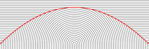
The proof of Proposition 3.2 will be given in [23]. When $\rho$ is given by (19), the jump set $\mathcal{C}$ can be described in Cartesian coordinates as the graph of

$x_2=\frac{L}{2}-\frac{x_1^2}{2L}\mathrm{f}\mathrm{o}\mathrm{r}-L\le x_1\le L.$

In particular, $\mathcal{C}$ is a parabolic arc (see Figure 6). It can be shown that, at each point, the normal to the curve $\mathcal{C}$ bisects the angle between the smectic layers.

Figure 6. (Colour online) The minimizing configuration given by Proposition 3.2. The black lines represent the smectic layers, while the thick red line is the jump set $\mathcal{C}$.

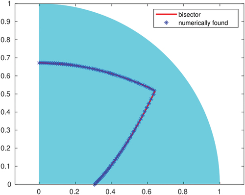
Next, we consider a domain, which is a quarter disk of unit radius, $\mathrm{\Omega }:=\{\mathbf{x}=(x_1,x_2)\in {\mathbb{R}}^2:x_2^2+x_2^2<1,x_1>$

$0,x_2>0\}$. Again, we minimise within a restricted class of configurations, whose jump set has the form

(20) $\mathcal{C}=\left\{(\rho (\theta )cos\theta ,\rho (\theta )sin\theta ):0\le \theta \le \frac{\pi }{2}\right\}$(20)

The function $\rho$ is unknown but, in contrast to the previous example, the boundary values $\rho (0)$, $\rho (\pi /2)$ are unspecified. We consider maps $\mathbf{Q}$ of the form (18), where the director $\mathbf{n}$ is given by

(21) $\mathbf{n}(rcos\theta ,rsin\theta ):=\left\{\begin{array}{cc}(0,1)& \mathrm{i}\mathrm{f}r<\rho (\theta ),0<\theta <\pi /2\\ (cos\theta ,sin\theta )& \mathrm{i}\mathrm{f}r>\rho (\theta ),0<\theta <\pi /2.\end{array}\right.$(21)

In particular, the layers are horizontal on the left side of $\mathcal{C}$ and circular on the right side. Moreover, we impose planar anchoring conditions near the boundary at $x_1=0$, defined in terms of the director as $\mathbf{n}(x_1,x_2)=(1,0)$ for $x_2<0$. As a result, the jump set of $\mathbf{Q}$ contains an additional component on the boundary of $\mathrm{\partial }\mathrm{\Omega }$, i.e. the straight-line segment with endpoints $(0,0)$ and $(0,\rho (0))$, where the director jumps from the value $(1,0)$ to $(0,1)$. In the energy functional, we account for this additional contribution as well. Moreover, in this example, we do not neglect the elastic energy.

Figure 7 shows a numerical approximation of the minimiser of (17) within this restricted class, for $K_1=2$ and different values of $\alpha$, $\mu$. The simulation is based on a MATLAB code, and the details are provided in Appendix A. The numerical method we use is not guaranteed to converge to a global minimum of the problem. However, we repeated the simulations using several different initial guesses for $\rho$, including random ones, and obtained qualitatively similar profiles for the jump set. The numerically found jump set very nearly agrees with a union of two parabolic arcs that bisect the smectic layers at each point, given explicitly as

Figure 7. (Colour online) Numerics for the problem on a quarter circle. All the pictures have $K_1=2$.

(22) $x_1=min\left({\left(a^2+2a{x}_2\right)}^{1/2},{\left(b^2-2b{x}_2\right)}^{1/2}\right)$(22)

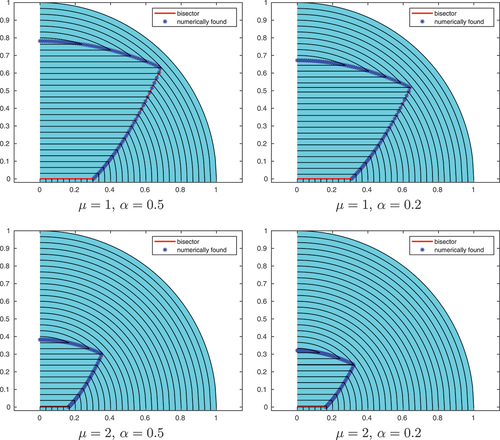
for some positive numbers $a$, $b$. In Figure 7, we compare the numerical solution with the parabolic arcs given by (22), where we have chosen the parameters $a$, $b$ so as to match the boundary values of the numerically found solution; the difference between the two curves is almost unnoticeable. Numerical tests show that the jump set tends to shrink towards the centre of the circle as $\mu$ increases or $\alpha$ decreases, although the dependence on $\alpha$ seems to be weaker. This is consistent with the fact that the jump energy density is monotonically increasing as a function of $\mu$ and decreasing as a function of $\alpha$. Therefore, as $\mu$ increases or $\alpha$ decreases, energy minimisation requires the jump set to become shorter, in order to compensate for the larger values of the jump energy density.

4. Discussion and future directions

In this paper, we have shown how a free discontinuity model has the potential to describe the configurations of smectic A layers observed in thin-film experiments. An advantage of free discontinuity models in this context is that they represent defect walls as sharp interfaces with precise locations. However, our analysis is just a beginning and much remains to be done. In particular, we are currently unable to formulate the thin-film problem as a well-posed free-boundary problem in either two or three dimensions, so that the profile of the upper free surface and the width of the oily streaks can be predicted.

Of course, it would be physically relevant to consider three-dimensional free discontinuity problems. The conditions (C1)–(C3) are still meaningful in three dimensions, up to a few obvious modifications. (As a side remark, assuming that the three-dimensional energy density is invariant with respect to the action of rotations $\bar{\mathbf{R}}\in \mathrm{S}\mathrm{O}(3)$ only is enough to guarantee that, in the two-dimensional case, the condition (C3) is satisfied for any $\mathbf{R}\in \mathrm{O}(2)$. Indeed, any $\mathbf{R}\in \mathrm{O}(2)$ can be realised as a $(2\times 2)$-submatrix of a three-dimensional rotation $\bar{\mathbf{R}}\in \mathrm{S}\mathrm{O}(3)$.) The definition of BV-ellipticity, too, extends to higher dimensions with no essential change (see, e.g. [18], Definition 5.13 for the details). However, the condition (C4) needs more substantial modifications, because (10) (or equivalently, (11)) is not enough to avoid dislocations of the smectic layers at the defect walls in three dimensions. In order for the layers to be consistently defined across a defect wall, the unit normal $\mathit{\nu }$ to the jump set and the molecular directors ${\mathbf{n}}^{+}$, ${\mathbf{n}}^{-}$ on either side of the jump, must satisfy (10) and, additionally, they must be coplanar. (If ${\mathbf{n}}^{+}$, ${\mathbf{n}}^{-}$ and $\mathit{\nu }$ are not coplanar, then the intersection lines between the layers on either side do not belong to the jump set and, hence, dislocations arise.) The singular energy density ${\zeta }_{\alpha }$, defined in (12), needs to be modified accordingly. Finally, the energy density ${\phi }_{\alpha }$ is still well defined in three dimensions, as (14) remains meaningful. However, we do not know whether the three-dimensional analogue of ${\phi }_{\alpha }$ is the BV-elliptic envelope of the three-dimensional analogue of ${\zeta }_{\alpha }$, nor whether it is BV-elliptic at all, because our arguments in [23] do not apply to the three-dimensional case.

Analytic work on these problems would need to be supplemented by numerical studies, and there is a need to develop appropriate numerical methods for freediscontinuity (and free boundary) problems associated with jump energy densities of the type (14). Such jump energies also need further study, and it would be useful to broaden the class of BV-elliptic jump energies satisfying (C1)–(C4) in particular, to allow different minima at the two angle bisectors.

Finally, it is important to understand the relation between models based on a molecular density and our ‘sharp interface’ model. In this context, there are interesting numerical computations of Xia, Maclachlan, Atherton & Farrell [24] using a modification of a model of Ball & Bedford [10], which is in turn based on that of Pevnyi, Selinger & Sluckin [25].

Acknowledgments

We would like to thank Emmanuelle Lacaze for many very helpful discussions. We also thank Giacomo Albi and Marco Caliari from the University of Verona for their help with the numerical simulations, and the referee for their careful reading of the manuscript and comments.

Disclosure statement

No potential conflict of interest was reported by the author(s).

Data availability statement

Data sharing is not applicable to this article as no new data were created or analysed in this study.

Notes

1. In [23], we will show that ${\phi }_{\alpha }$ is not only BV-elliptic, but also jointly convex, in the sense of [18], Definition 5.17. Joint convexity is a sufficient condition for BV-ellipticity, but it is not known whether it is a necessary condition as well.

Appendix A.

Numerical simulations

In this section, we present the details of the numerical simulations for the minimisation problem on a quarter circle, described in Section 3. The $\mathbf{Q}$-tensor is defined in terms of a scalar function $\rho :[0,\pi /2]\to \mathbb{R}$, as in (18), (21). However, we find it convenient to introduce a new variable $u=u(\theta )$, defined by

(23) $\rho (\theta )=e^{-u(\theta )}\mathrm{f}\mathrm{o}\mathrm{r}\mathrm{a}\mathrm{n}\mathrm{y}0<\theta <\frac{\pi }{2}.$(23)

The original variable $\rho$ is subject to the geometric constraints $0<\rho <1$, because the domain is a quarter circle of unit radius. However, we minimise numerically the energy functional subject to no constraints on $u$. Equation (23)(23) $\rho (\theta )=e^{-u(\theta )}\mathrm{f}\mathrm{o}\mathrm{r}\mathrm{a}\mathrm{n}\mathrm{y}0<\theta <\frac{\pi }{2}.$(23) guarantees that $\rho >0$, but for some values of $\alpha$, $\mu$ (not shown in Figure 7), we did find numerical solutions that are not admissible, because they do not satisfy $\rho <1$.

The energy can be written as a functional of $u$ by a direct computation, using (18), (21) and (23). The energy consists of a sum of three terms:

(24) $I(u)=I^{\mathrm{e}\mathrm{l}}(u)+I^{\mathrm{j}\mathrm{u}\mathrm{m}\mathrm{p},\mathrm{i}\mathrm{n}\mathrm{t}}(u)+I^{\mathrm{j}\mathrm{u}\mathrm{m}\mathrm{p},\mathrm{b}\mathrm{d}}(u)$(24)

The first term, $I^{\mathrm{e}\mathrm{l}}(u)$, is the elastic energy:

(25) $\begin{array}{rl}& I^{\mathrm{e}\mathrm{l}}(u):=\frac{K_1}{2}{\int }_{\mathrm{\Omega }}{\left|\mathrm{\nabla }\mathbf{Q}(\mathbf{x})\right|}^2\mathrm{d}\mathbf{x}=\frac{K_1}{2}{\int }_0^{\pi /2}\left({\int }_{e^{-u(\theta )}}^1\frac{\mathrm{d}\rho }{\rho }\right)\mathrm{d}\theta \\ & =\frac{K_1}{2}{\int }_0^{\pi /2}u(\theta )\mathrm{d}\theta \end{array}$(25)

The second term, $I^{\mathrm{j}\mathrm{u}\mathrm{m}\mathrm{p},\mathrm{i}\mathrm{n}\mathrm{t}}(u)$, is the contribution to the jump energy from the curve $\mathcal{C}$, given in (20):

(26) $\begin{array}{rl}& I^{\mathrm{j}\mathrm{u}\mathrm{m}\mathrm{p},\mathrm{i}\mathrm{n}\mathrm{t}}(u):=\mu {\int }_C\phi ({\mathbf{Q}}^{+},{\mathbf{Q}}^{-},\nu )d{H}^1\\ & =\mu {\int }_0^{\pi /2}{\left|cos\theta \right|}^{\alpha }{e}^{-u(\theta )}{\left.\left(\begin{array}{c}{u}^{\mathrm{\prime }}{(\theta )}^2+1\\ \left.+\left|f(\theta ,u^{\mathrm{\prime }}(\theta ))\right.\right|\end{array}\right.\right)}^{1/2}\mathrm{d}\theta \end{array}$(26)

with

(27) $f(\theta ,u^{\mathrm{\prime }}(\theta )):=(u^{\mathrm{\prime }}(\theta {)}^2-1)cos\theta +2u^{\mathrm{\prime }}(\theta )sin\theta$(27)

The expression (26)–(27) is deduced from (15), by applying trigonometric identities to simplify the form of the integrand. The integrand in (26) is not differentiable at the points where $f(\theta ,u^{\mathrm{\prime }}(\theta ))=0$. As the numerical minimisation is based on a quasi-Newton method, which works best for differentiable functions, we regularise the integrand by introducing a parameter $\epsilon >0$:

(28) $\begin{array}{rl}& I^{\mathrm{j}\mathrm{u}\mathrm{m}\mathrm{p},\mathrm{i}\mathrm{n}\mathrm{t}}(u)\approx \mu {\int }_0^{\pi /2}{\left|cos\theta \right|}^{\alpha }{e}^{-u(\theta )}(u^{\mathrm{\prime }}(\theta {)}^2+1\\ & +(\epsilon +f(\theta ,u^{\mathrm{\prime }}(\theta ){)}^2{)}^{1/2}{)}^{1/2}\mathrm{d}\theta \end{array}$(28)

The pictures in Figure 7 are obtained for $\epsilon ={10}^{-12}$. Finally, $I^{\mathrm{j}\mathrm{u}\mathrm{m}\mathrm{p},\mathrm{b}\mathrm{d}}(u)$ is the contribution to the jump energy from jumps that are located on the boundary of $\mathrm{\Omega }$ — more precisely, on the line segment $S$ with endpoints $(0,0)$ and $(0,\rho (0))$:

(29) $\begin{array}{cc}{I}^{\mathrm{j}\mathrm{u}\mathrm{m}\mathrm{p},\mathrm{b}\mathrm{d}}(u)& :=\mu {\int }_S\phi ({\mathbf{Q}}^{+},{\mathbf{Q}}^{-},\mathit{\nu })\mathrm{d}{\mathcal{H}}^1=\sqrt{2}\mu e^{-u(0)}\end{array}$(29)

This term can also be written in integral form, by considering a smooth function $g:[0,\pi /2]\to \mathbb{R}$ such that $g(0)=1$, $g(\pi /2)=0$ and writing

(30) $\begin{array}{cc}{I}^{\mathrm{j}\mathrm{u}\mathrm{m}\mathrm{p},\mathrm{b}\mathrm{d}}(u)& =-\sqrt{2}\mu {\int }_0^{\pi /2}\frac{\mathrm{d}}{\mathrm{d}\theta }\left(e^{-u(\theta )}g(\theta )\right)\mathrm{d}\theta \\ \hspace{0.17em}& =\sqrt{2}\mu {\int }_0^{\pi /2}{e}^{-u(\theta )}\left(u^{\mathrm{\prime }}(\theta )g(\theta )-g^{\mathrm{\prime }}(\theta )\right)\mathrm{d}\theta \end{array}$(30)

We found that, when writing the boundary term in the form (29), the numerical solution deviates from the parabolic arcs (22) near $\theta =0$. However, the thickness of this ‘boundary layer’ is mesh-dependent, so this feature is probably a numerical artifact. The pictures in Figure 7 are obtained by considering the integral form (30) of $I^{\mathrm{j}\mathrm{u}\mathrm{m}\mathrm{p},\mathrm{b}\mathrm{d}}$, with $g(\theta ):=1-2\theta /\pi$, and present no boundary layer. Other choices of the function $g$, e.g. $g(\theta ):=cos\theta$, produce qualitatively similar profiles for the jump set.

We discretise the functional (24) on a uniform mesh of $m$ points in $[0,\pi /2]$. We approximate the derivative $u^{\mathrm{\prime }}(\theta )$ by second-order central finite differences, and we approximate the integrals by the trapezoid rule. The number $m$ of mesh points is increased gradually, from $m=50$ to $m=100$. At each step of the iteration over $m$, we call the built-in MATLAB function fminunc, which applies the Broyden-Fletcher-Goldfarb-Shanno Quasi-Newton algorithm to minimise the functional (24) under no constraints on $u$. The initial guess for the minimisation process is defined by the numerical minimiser found at the previous step.

References

- Michel JP, Lacaze E, Alba M, et al. Optical gratings formed in thin smectic films frustrated on a single crystalline substrate. Phys Rev E. 2004;70(1):011709.
- Michel JP, Lacaze E, Goldmann M, et al. Structure of smectic defect cores: X-ray study of 8CB liquid crystal ultrathin films. Phys Rev Lett. 2006 Jan;96:027803.
- Zappone B, Lacaze E. Surface-frustrated periodic textures of smectic-A liquid crystals on crystalline surfaces. Phys Rev E. 2008 Dec;78:061704.
- Zappone B, Meyer C, Bruno L, et al. Periodic lattices of frustrated focal conic defect domains in smectic liquid crystal films. Soft Matter. 2012;8:4318–4326.
- Coursault D, Zappone B, Coati A, et al. Self-organized arrays of dislocations in thin smectic liquid crystal films. Soft Matter. 2016;12(3):678–688. Available from: https://pubs.rsc.org/en/content/articlelanding/2016/sm/c5sm02241j
- Zappone B, Lacaze E. One-dimensional patterns and topological defects in smectic liquid crystal films. Liq Cryst Rev. 2022;1–18. DOI:10.1080/21680396.2022.2076748
- Jeridi H, et al. Unique orientation of 1D and 2D nanoparticle assemblies confined in smectic topological defects. Soft Matter. 2022;18:4792–4802. DOI:10.1039/d2sm00376g.
- De Giorgi E, Ambrosio L. Un nuovo funzionale nel calcolo delle variazioni. Atti Accad Naz Lincei Rend Cl Sci Fis Mat Nat (8). 1988;82(2):199–210. (1989).
- Francfort GA, Marigo JJ. Revisiting brittle fracture as an energy minimization problem. J Mech Phys Solids. 1998;46(8):1319–1342.
- Ball JM, Bedford SJ. Discontinuous order parameters in liquid crystal theories. Mol Cryst Liq Cryst. 2015;612(1):1–23.
- Oseen CW. The theory of liquid crystals. Trans Faraday Soc. 1933;29:883–899.
- Leslie FM, Stewart IW, Nakagawa M. A continuum theory for smectic C liquid crystals. Mol Cryst Liq Cryst. 1991;198(1):443–454.
- de Gennes PG. An analogy between superconductors and smectics A. Solid State Commun. 1972;10(9):753–756.
- Chen JH, Lubensky T. Landau-Ginzburg mean-field theory for the nematic to smectic-C and nematic to smectic-A phase transitions. Phys Rev A. 1976;14(3):1202.
- Kléman M, Parodi O. Covariant elasticity for smectics A. J Phys. 1975;36(7–8):671–681.
- Han J, Luo Y, Wang W, et al. From microscopic theory to macroscopic theory: a systematic study on modeling for liquid crystals. Arch Ration Mech Anal. 2015;215(3):741–809.
- Ball JM. Mathematics and liquid crystals. Mol Cryst Liq Cryst. 2017;647(1):1–27.
- Ambrosio L, Fusco N, Pallara D. Functions of bounded variation and free discontinuity problems. New York: The Clarendon Press, Oxford University Press; 2000.
- Ambrosio L, Braides A. Functionals defined on partitions of sets of finite perimeter, I: integral representation and Γ-convergence. J Math Pures Appl. 1990;69:285–305.
- Ambrosio L. Existence theory for a new class of variational problems. Arch Rational Mech Anal. 1990;111(4):291–322.
- Ambrosio L, Braides A. Functionals defined on partitions in sets of finite perimeter II: semicontinuity, relaxation and homogenization. J Math Pures Appl. 1990;69:307–333.
- Caraballo D. BV-ellipticity and lower semicontinuity of surface energy of Caccioppoli partitions of ℝn. J Geom Anal. 2013;23:202–220.
- Ball JM, Canevari G, Stroffolini B. Analysis of a free discontinuity model for smectic thin films. To appear.
- Xia J, MacLachlan S, Atherton TJ, et al. Structural landscapes in geometrically frustrated smectics. Phys Rev Lett. 2021 Apr;126(17):177801.
- Pevnyi MY, Selinger JV, Sluckin TJ. Modeling smectic layers in confined geometries: order parameter and defects. Phys Rev E. 2014 Sep;90:032507.