Macrofinancial linkages and income distribution in the South African economy

ABSTRACT

This study examines the impact of financial factors and income distribution on aggregate demand and growth in South Africa, using data spanning 1980–2019. We applied the autoregressive-distributed-lag bounds-testing procedure to uncover the effects over the short-and-long-run horizons. Additionally, we estimated impulse response functions to reveal further dynamic interactions. Our findings indicate that the key financial factors affecting the South African real economy are credit growth, interest rates, house prices and exchange rates. House prices play an important role, via the collateral channel, in driving consumption demand. Meanwhile, credit growth stifles investment demand in the long run. Interest rates constrain demand and growth, while the strengthening of exchange rates improves investment for firms. However, exchange rates impact negatively on GDP, presumably, through the trade-channel. We also found that income inequality suppresses consumption and investment demand, as well as GDP. This suppression appeared to be relatively pronounced in the short run for investment and growth, while for consumption, the suppressive impact was persistent. Therefore, we recommend that any policy framework aiming to galvanise growth should not overlook the problem of inequality. Otherwise, any headway made on growth will be back-pedalled by the demand-reducing impact of high-income inequality.

KEYWORDS:

• Macro-financial linkages
• income distribution
• real economy
• finance
• income inequality
• South Africa

JEL CLASSIFICATION:

• E44
• D31
• D33

1. Introduction

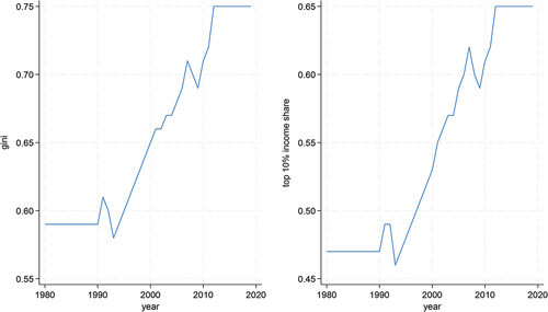
Inequality in South Africa has deep historical and political roots (Terreblanche 2002). However, the post-apartheid period paints a very grim picture of the status of income inequality in the country. The distribution of income since the mid-1990s is characterised by steep rises in both the Gini coefficient and the share of income in the top decile (see Figure 1 below). According to various survey-data-based estimates, the Gini coefficient for South Africa ranged between 0.66 and 0.72 between the years 1993 and 2015 (Hundenborn, Leibbrandt, and Woolard 2018; StatsSA (Statistics South Africa) 2019). It is also shown that since 1994 the top decile of the income distribution has moved further up from the middle, while the bottom has fallen behind (Wittenberg 2017).

Figure 1. Plots of the Gini index (left) and the top 10% income share (right), for the period 1980–2019.

The plots are based on data from the World Inequality Database.

A growing number of studies that analyse household and labour survey data, as well as income tax data, have identified labour market earnings inequality as the primary driver of overall income inequality in South Africa since the early 1990s (Bassier and Woolard 2021; Finn and Leibbrandt 2018; Hundenborn, Leibbrandt, and Woolard 2018; Leibbrandt, Finn, and Woolard 2012; Wittenberg 2017). This is because labour market income constitutes the largest share of total household income. Meanwhile, although real earnings have risen since the 1990s, the top of the income distribution has amassed the largest proportion of the income growth, while the middle has seen relatively low-income growth over the past two decades (Finn and Leibbrandt 2018).

The substantial growth of top incomes has been partly attributed to several features that have accompanied the evolution of the domestic labour market. These include, on the one hand, the skill-bias technical change that has potentially favoured those at the top of the income distribution who are more likely to be highly skilled and thus possess greater bargaining power (Bassier and Woolard 2021). On the other hand, the decline in employment in sectors such as agriculture, manufacturing and mining over the past two decades has negatively impacted the incomes (and employability) of the less skilled who occupy the bottom of the income distribution (Leibbrandt, Ranchhod, and Green 2021).¹

The recent financial crisis of 2007–2009 led some scholars to assert that rising inequality is at the root of historic and recent financial crises, citing the significant rises in top income shares that preceded the Great Depression and the Great Recession (e.g. Kumhof, Rancière, and Winant 2015; Stockhammer 2015). The main argument is that rising inequality suppresses aggregate demand as resources are redistributed from low-to-middle income households with a high marginal propensity to consume (MPC) to high-income households with a low MPC. Consequently, high MPC households increase their indebtedness to maintain consumption. The argument goes further to ascribe an amplifying role to lenient regulation and low interest rates, aimed at reviving aggregate demand, which make way for excessive debt accumulation, thereby creating conditions of macro-financial fragility.

This proposed linkage among inequality, credit and aggregate demand prompts the notion that income distribution may be playing an integral role in macro-financial interactions. Indeed, there have been recent attempts to treat this linkage formally and propose hypotheses as to how the interactions occur. For instance, some studies evoke the relative consumption assumption, suggesting that a certain group of consumers emulate the consumption standards of those above them in the income distribution. Due to their lower income share, these consumers engage in credit which then fuels a debt-financed consumption boom (Kapeller and Schütz 2014, 2015).

Apart from these few examples, extant literature has treated this topic in a largely fragmented manner. That is, some sections of the literature focus on the income distribution and real economy nexus, whereas others focus on inequality and finance. Moreover, although the literature appears to confirm some effects of income inequality on finance and the macroeconomy, the related empirical evidence is mixed. This leaves a gap in the literature that warrants more comprehensive and integrated assessments of the impact of income distribution, in conjuction with financial factors, on the macroeconomy. This study utilises a unified framework that marries macro-finance literature with various perspectives on the effects of income distribution.

To provide a bit of context for the macro-finance and income distribution nexus, it is worth mentioning that recent evidence suggests a negative correlation between income inequality and durations of positive economic growth (Berg and Ostry 2017). This implies that it is difficult to achieve longer durations of growth under conditions of high-income inequality. To explore the possible channels through which inequality can retard the sustainability of growth, we may tap into some related theoretical propositions. For instance, credit market imperfections are posited to be more pronounced for small borrowers with lower net worth (Bernanke, Gertler, and Gilchrist 1996). Consequently, if a large population of low-income households and small firms suffer constrained access to finance, consumption and investment demand as well as cycles of growth are less likely to be sustained. Even with wider credit access, theoretical studies also predict that income inequality can lead to high levels of indebtedness amongst those below the top decile of the income distribution as they strive to keep up with consumption standards (Kapeller and Schütz 2014, 2015). This indebtedness in turn can precipitate defaults, hinder access to additional finance (e.g. through credit rationing), and erode future income due to high debt repayments that stifle demand (Kapeller and Schütz 2014; Palley 1994). As aggregate demand is stifled, investing firms’ profit margins decline (Ryoo 2016), discouraging further investment to sustain profitability.

Therefore, this study contributes to the existing literature by providing empirical support for the theoretical propositions that attempt to link the three phenomena that concern this study, namely, inequality, finance and the real economy. Our case study of the South African economy is particularly pertinent for two reasons. Firstly, there has been scant attention paid to macro-financial linkages in the South African context, let alone to the influence of income distribution thereon. Secondly, South Africa has experienced a significant rise in income inequality in recent decades, which has coincided with struggles to sustain lengthy periods of substantial economic growth and high investment rates since the mid-1990s (Driver and Harris 2021; Du Plessis and Smit 2009). This is despite the country’s significant financial depth in terms of the banking sector (Hawkins 2021).

The rest of the paper proceeds as follows: Section 2 presents our conceptual framework which guides our empirical methods and analysis. In Section 3, we outline the data and empirical methods that were used in the study. Section 4 presents and discusses the results, while Section 5 provides a summary of the study’s findings and concludes the paper.

2. Conceptual framework

Our conceptual framework relies on theoretical insights from the literature on macro-financial linkages and the impact of income distribution. From the macro-finance point of view, we draw on Minsky’s ([1982]2016; 1986) seminal work, which focuses on endogenous interactions between financial cycles and economic fluctuations. In his work, Minsky referred to swings in the financial system that endogenously drive economic fluctuations. A key proposition is that good economic times, associated with high cash flows and asset prices, stimulate positive long-term expectations about the economy, which justify lower margins of safety by lenders and higher leverage ratios by firms seeking to increase investment. However, this creates conditions of fragility, as higher interest rates can make it difficult for firms to fulfil debt obligations, leading to tighter financing conditions, reduced investment, and economic contraction.

Minsky’s work inspired a stream of contributions that attempt to model macro-financial interactions, for both household and firm sectors (e.g. Fazzari, Ferri, and Greenberg 2008; Kohler 2019; Palley 1994; Ryoo 2013). Some of the recent theoretical contributions in this line of literature also provide plausible propositions on how income inequality may be playing an integral role in real-financial interactions (Kapeller and Schütz 2014, 2015). For other insights on distributional effects, we additionally draw on the Kaleckian literature, which focuses on the impact of functional income distribution on the components of aggregate demand (Blecker 2002, 2016; Carvalho and Rezai 2016; Palley 2017).

Consistent with the Minskyan (also Keynesian and Kaleckian) perspective, we take it that real economic activity is demand-driven. Accordingly, we measure the real sector by investment demand $\mathbf{I}$, and consumption demand $\mathbf{C}$. We abstract from the government sector and focus specifically on private sector demand and the linkages with financial and distributional factors. We further abstract from the external sector in the sense of imports and exports. Instead, we proxy for external effects by the exchange rate which we think is a more relevant variable for real-financial interactions (Rey 2016). Below, we present our investment and consumption functions, which will in turn inform our empirical analysis in the subsequent sections.²

2.1. Investment

(1) $\mathbf{I}=\mathrm{f}(\mathrm{Ygdp},\mathrm{CRED},\mathrm{SPI},\mathrm{INTR},\mathrm{EXR},\mathrm{INCOME}10,\mathrm{PS},\mathrm{ROP})$(1)

(1) states that investment demand ($\mathbf{I}$) is a function of output growth, financial factors, and distributional variables; namely, real GDP (Ygdp), credit (CRED), stock prices (SPI), interest rates (INTR), exchange rates (EXR), income inequality (INCOME10), the profit share (PS) and the rate of profit (ROP). The GDP variable is meant to capture the accelerator effects which relate the level of investment to the rate of change in output growth (Blecker 2016; Chirinko, Fazzari, and Meyer 1999). This association may be expected to be relatively more pronounced in the long-term than in the short run. This is because cash flows and profitability affect the current fluctuations in investment spending, while longer-term capital accumulation primarily depends on the trajectory of the economy (i.e. output growth) and on the variations in the cost of capital (Blecker 2016; Chirinko, Fazzari, and Meyer 2011).

The financing of investment is sourced both internally and externally, hence the credit variable in our investment function represents access to external finance (Minsky 1975). Since debt accumulation by firms may constrain continued investment spending due to increased cash-flow commitments to creditors (Fazzari, Ferri, and Greenberg 2008; Minsky 1986), credit will have a positive effect in the short-run but can potentially exert a negative effect on investment demand over the longer-term. The negative effect of credit may signal a cyclical downturn in the economy.

Another important factor related to external finance is the interest rate. Interest rates matter for investment in at least two ways. First, they represent the cost of capital, such that when they are high, it is difficult to borrow and finance investment. Second, changes in interest rates affect the service costs of existing debt through interest expenses. Through their effect on the debt service burden, high interest rates reduce internal cash flows and precipitate a downturn in investment activity (Fazzari, Ferri, and Greenberg 2008).

Stock prices represent the market valuation of the capital assets that are held in firms. These prices are determined by discounting expected future cash-flows to the present. Thus, high asset prices would be indicative of high expected cash-flows, and thereby, would positively affect the demand for investment (Minsky [1982]2016).

Moreover, the exchange rate variable captures the sensitivity of investment to changes in the local currency movements. This is because currency depreciations deter investment expenditure as they weaken the balance sheets of externally indebted firms in that more foreign currency would be required to pay the interest costs that are magnified by a weaker currency (Kohler 2019). Thus, we expect that an appreciation of the local currency will impact positively on investment demand.

The distributional variables include the profit share, and the income share that goes to the top 10% in the income distribution. The profit share is both an internal cash-flow variable and a distributional variable. As an internal cash-flow variable, the profit share represents retained earnings, after accounting for such expenses as depreciation, taxes, interest payments and dividend pay-outs (Blecker 2016). These net earnings are the base upon which debt can be sought to finance investment (Minsky 1975). As such, they alleviate financing constraints and enable firms to pursue desired investment. The profit share is also a distributional variable in the sense that it can be reduced by a higher wage share, resulting in lower internal cash-flows for investment (Fazzari, Ferri, and Greenberg 2008). In that sense, the profit share also influences the debt dynamics of the firm because a higher share reduces the rate of debt accumulation for the firm, as more internal funds would be available.

The other key distributional factor is the top 10% income share. Assuming positive saving out of labour income (Palley 2017) and a rising propensity to save from the bottom to the top of the income distribution (Carvalho and Rezai 2016), a greater share of the income accruing to the top decile implies a higher savings rate. It follows that the effect on investment demand should be positive due to higher aggregate saving.

Finally, the effect of profitability on investment demand may additionally operate via the rate of profit (Palley 2017). This idea derives from Marglin and Bhaduri’s (1991) proposition that, even if the profit share is squeezed and the wage share is higher, the rate of profitability can still be raised. This is because firms can increase their mark-ups to realise the profits, thereby enabling further investment spending (Blecker 2002). In addition, the profit rate can also be construed as the rate of return on investment. Therefore, the purpose of our rate of profit variable is to encapsulate these additional roles of profitability in investment demand.

2.2. Consumption

(2) $\mathrm{C}=\mathrm{f}(\mathrm{CRED},\mathrm{HPI},\mathrm{SPI},\mathrm{INTR},\mathrm{INCOME}10,\mathrm{WS},\mathrm{PS})$(2)

Consumption would in the first instance depend upon income, hence we have labour-income (i.e. the wage share, WS) as well as capital-income (i.e. the profit share, PS). In addition to income, consumption is influenced by house prices (HPI), stock prices (SPI), interest rates (INTR), credit (CRED) and income inequality (INCOME10). The positive effect of the $\mathrm{WS}$ on consumption can be expected to be more significant than the effect of the $\mathrm{PS}$, under the assumption that the MPC out of labour income is higher than out of capital income. This is because capital income consists of profits, a great part of which is retained by firms, and wealth, such as interest and dividend income, which mostly accrues to top-income-households who have higher saving propensities (Blecker 2016).

In addition to the functional distribution of income, we include personal income distribution. Since MPCs are lower at the top of the income distribution, high income inequality would impact negatively on consumer demand. However, if top-income-households have a propensity to save that is not (much) stronger than their MPC, there is increased likelihood of consumption inequality. Now, the presence of consumption inequality invokes the possibility that lower-income-households will increase their credit demand to keep up with consumption standards (Ryoo and Kim 2014). That is, if lower-income-households have consumption desires that exceed their incomes, they will borrow to meet these desires, and thereby give rise to a borrowing-supported expansion in consumer demand.

However, borrowing itself redistributes income from lower-income-households to the top-income-households through interest costs, while accumulated debt stifles further borrowing and eats up future income through repayments (Palley 1994; Ryoo and Kim 2014). We, therefore, expect that, on the one hand, distributional factors, including income inequality, will have effects that are more likely to be significant in the longer run. This is because households tend to maintain steady consumption behaviours in the face of short-run income fluctuations (Blecker 2016), possibly using credit arrangements. On the other hand, we anticipate that the impact of credit is mostly positive in the short run but may turn negative over time due to the impact on income of the burden of accumulated debt.

Turning now to the financial factors. Through the collateral channel, the effect of house prices on consumption can be expected to be positive. This is because a rise in house prices represents an increase in the wealth of house-owning households. As such, increased wealth improves borrowing capacity and stimulates consumer demand (Ryoo 2016). However, since accumulated debt reduces future income, and house prices are subject to change, the housing wealth effects may still turn insignificant over time. In addition, interest rates would also exert a negative impact on consumer demand as they increase interest expenses on existing debt and deter the uptake of new credit.

Finally, the inclusion of the stock price variable is to account for the possibility that there may be capital-income-earning households that have saving propensities that do not significantly exceed their consumption desires out of their capital income. In which case, stock price booms would impact positively on consumption demand (Ryoo 2010, 2013). We now proceed to outline the data and the empirical methods used in the study.

3. Data and methods

3.1. Data

The study uses South African data covering the period 1980–2019. The sample period was primarily determined by data availability; otherwise, we would have preferred a period that extends to the COVID-19 era. Nevertheless, the chosen period still encompasses much of the post-apartheid era, which saw a sustained rise in income inequality. The data were obtained from the South African central bank and other global sources (see Table A1 in the Appendix).

Our dataset encompasses the real and financial sectors, as well as distributional factors. For the real sector, we utilised (i) gross fixed capital formation and (ii) final household consumption expenditure, both scaled by real GDP. According to Borio (2014), financial cycles are driven by financing constraints, such as access to credit, and by perceptions of risk and value, as reflected in asset prices. Therefore, we proxied the financial sector using domestic credit extended to the private sector (scaled by GDP), house price indices, and stock price indices. Nominal exchange rates captured the effects of currency movements. Lastly, long-term interest rates served as a measure of the cost of external finance, as their duration aligns closely with capital expenditures and durable consumption goods.

Regarding distributional factors, we measured income inequality using the top 10% income share. This is because the widening of income inequality in South Africa is primarily driven by the rise of top earnings (Bassier and Woolard 2021; Wittenberg 2017). We also employed profit and wage shares, the relevance of which goes back to the notion of differential marginal propensities to consume out of wage income and capital income (Kalecki 1954). The wage share is measured by the compensation-of-employees-to-GDP ratio (at factor cost). Following Stockhammer (2017), we adjusted this measure to exclude public labour income, as the government sector does not have a profit share, unlike private enterprises.³ Finally, the rate of profit is measured by country-level profit rates, calculated as net profit income divided by capital stock (Basu et al. 2022).

3.2. Estimation methods

The empirical analysis was primarily conducted using the ARDL bounds-testing approach (Pesaran, Shin, and Smith 2001). This was because our conceptual framework suggested short-and-long-term dimensions in the interactions among the key variables of the study. Thus, the ARDL framework was chosen because of its capability to unearth the dynamics that take place in both these time horizons. We also chose this method due to its features which made it more accommodative for the current study than other comparable methods. For instance, the ARDL procedure can handle variables of purely I(0), I(1), or the combination of both, which lends itself well to the mixed order of integration that characterised our time series. Moreover, the ARDL method has been shown to provide robust results even when the sample size is relatively small (Pesaran, Shin, and Smith 2001; Narayan 2005). However, our 8-variable models may be considered large for an ARDL which estimates only one error correction term per model. In which case, a vector error correction (VEC) model makes an ideal alternative because it does not only estimate both short-and-long dynamics but can also provide multiple cointegration vectors in a single model.⁴ However, the VEC model can still be over-parameterised due to a limited number of observations, as in our study. Therefore, given the compatibility of the ARDL method with our small sample size and the stationary properties of our time series, we deemed it suitable for the study.

Technically, the ARDL method tests the significance of lagged variables in their levels under the null hypothesis that the long-run coefficients are equal to zero, indicating the non-existence of a level (long-run) relationship among the variables. The alternative hypothesis is that a level relationship exists. If the null is rejected, the long-run model is estimated, along with a restricted error correction model, to obtain long-run and short-run effects. The bounds-testing approach relies on an F-statistic which is computed and observed against critical values that have an upper bound and a lower bound. The upper bound critical values assume that the explanatory variables are all integrated of order one [I(1)], while the lower bound values assume that the regressors are all integrated of order zero [I(0)]. If the computed F-statistic lies within these bounds, the inference of a level relationship is inconclusive. However, if the F-statistic lies outside the bounds, the null hypothesis of a no level relationship can be either rejected (that is, when the F-statistic is greater than the upper bound), or not rejected, (in which case the F-statistic falls below the lower bound).

Prior to applying this method, we carried out unit root tests to ensure that none of our time series was integrated of an order higher than I(1), which the ARDL procedure does not permit. To this end, we utilised the Dicker-Fuller Generalised Least Squares (DF-GLS) test by Elliott, Rothenberg, and Stock (1996). Additionally, we used the Perron (1989, 1997) unit root with structural break test. We did so because macroeconomic time series, such as those used in this study, may have been affected by shocks in the past that led to structural shifts in the trend (or intercept) of the series.

The separate-equations approach, which we adopted by applying the ARDL framework sheds light on the dynamics that unfold over the short- and long-term horizons. However, this approach might not reveal all the dynamic interactions among the variables of interest. For example, we might be curious to know if income inequality negatively affects investment demand by suppressing consumption and aggregate demand, which would be unfavourable for profitability, or if inequality impacts investment positively, possibly through higher aggregate savings. To ensure that we do not miss out on other insightful cyclical interactions, we complementarily applied a system-of-equations approach.⁵ The additional approach treats all the study’s variables as endogenous variables that dynamically interact with one another through their lags, as in a vector autoregressive framework. The vehicle of estimation for this approach is the local projections method proposed by Jordà (2005). This method provides us with impulse response functions (IRFs) that show the response of each of our variables to a unit shock increase in another variable within the model. We now proceed to present and discuss the results of the empirical analysis.

4. Results and discussion

Before we delve into the main results, we examine the unit root tests outcomes which are presented in Table 1. Although only a few of the time series were stationary at levels, all of them became stationary after first differencing. A similar outcome was obtained when we applied a test that considers potential structural breaks in the time series. Since none of our series were integrated of an order beyond I(1), we proceeded to implement the bounds-testing procedure. For estimation purposes, we used the variables in their logarithmic form. The variables’ descriptive statistics are presented in Table B1 in the Appendix.

Table 1. Unit root test results.

		DF-GLS test				Unit root with breakpoint test
	Time series in levels		Time series in first differences		Time series in levels			Time series in first differences
Variables	Intercept	Intercept and trend	Intercept	Intercept and trend	Break in intercept	Break in trend	Break in both	Break in intercept	Break in trend	Break in both
LINV	−1.764*	−2.220	−3.736***	−3.852***	−3.949	−3.490	−3.075	−5.172**	−4.657**	−5.074
LCONS	0.368	−2.283	−4.839***	−5.355**	−4.857	−5.564***	−5.779***	−6.166***	−5.863***	−6.063***
LGDP	0.821	−1.954	−3.704***	−4.119***	−3.112	−2.586	−2.483	−5.675***	−5.675***	−5.714**
LCRED	0.078	−0.622	−1.437	−5.039***	−2.292	−2.899	−2.951	−5.165**	−4.992**	−5.025
LHPI	−2.319**	−2.831	−2.212**	−2.707	−4.775	−3.590	−4.562	−4.239	−4.052	−5.519**
LSPI	0.485	−3.191**	−5.123***	−6.146***	−3.994	−3.786	−4.253	−6.786***	−6.589***	−6.819***
LEXR	0.510	−1.435	−4.445***	−4.911***	−5.472***	−5.070***	−5.098	−5.574***	−5.214***	−6.241***
LINTR	−0.851	−1.890	−1.713*	−2.905*	−5.878***	−3.838	−4.520	−7.521***	−7.357***	−7.614***
LINCOME10	0.630	−1.752	−5.381***	−5.579***	−3.414	−2.328	−2.602	−7.537***	−6.108***	−7.875***
LWS	−2.152**	−2.086	−2.297**	−3.338**	−4.561	−4.292	−4.612	−5.004**	−4.931**	−5.138
LPS	−1.714*	−1.460	−1.834*	−2.951*	−4.574	−3.811	−4.614	−7.079***	−5.614***	−5.935***
LROP	−1.770*	−1.766	−2.048**	−3.018*	−3.267	−4.175	−5.076	−5.513***	−4.681**	−5.004

***, **, * indicate significance levels at 1%, 5% and 10% respectively. The variables are in logarithmic form and are defined as; LINV-investment, LCONS-consumption, LGDP-real GDP, LCRED-credit growth, LHPI-house prices, LSPI-stock prices, LEXR-exchange rates, LINTR-interest rates, LINCOME10-income inequality, LWS-wage share, LPS-profit share and LROP-rate of profit.

Source: Authors’ estimations using EViews.

Table 2 presents the investment and consumption models that we tested for the existence of cointegration, along with the results. The critical value bounds against which we checked the results of our F-tests (i.e. the bounds-tests) are shown in Table 3. As seen in Table 2, the F-test results confirm that the null hypotheses of no-cointegration were rejected for all the specified models. The F-statistics of both investment and consumption equations were significant at 1%. With cointegration confirmed, the next step was to estimate the long-run effects, as well as the short-run dynamics.

Table 2. Bounds-test results.

Outcome variable	Function	F-statistic	Outcome
Investment model
(1) LINV	f(LGDP, LCRED, LSPI, LINTR, LEXR, LINCOME10, LPS)	14.2854***	Cointegrated
(2) LINV	f(LGDP, LCRED, LSPI, LINTR, LEXR, LINCOME10, LROP)	11.4527***	Cointegrated
Consumption model
(1) LCONS	f(LCRED, LHPI, LSPI, LINTR, LINCOME10, LWS, LPS)	13.4241***	Cointegrated

***, **, * indicate significance levels at 1%, 5% and 10% respectively.

Source: Authors’ estimations using EViews.

Table 3. Critical values.

Significance level:	1%		5%		10%
No. of regressors:	k = 7		k = 7		k = 7
Bounds:	I(0)	I(1)	I(0)	I(1)	I(0)	I(1)
F-statistic
Sample size: n
35	3.841	5.686	2.753	4.209	2.300	3.606
40	3.644	5.464	2.676	4.130	2.260	3.534
Asymptotic	2.960	4.260	2.320	3.500	2.030	3.130

I(0) – lower nonstationary bound and I(1) – upper stationary bound. F-test critical values for 35–40 sample size obtained from Narayan (2005).

4.1. Long-run and short-run results

4.1.1. Investment results

Table 4 reports the long-run results for the investment models. We estimated two separate models for investment. The first model contains the profit share (LPS), while the second one includes the rate of profit (LROP) instead. This is because the rate of profit measure already embeds the profit share as one of its determinants (Basu et al. 2022). Therefore, the approach of separate equations was adopted to circumvent statistical inference problems that may arise because of perfect collinearity between the PS and the ROP.

Table 4. Long-run investment results: LINV.

Variable	Coefficient		Std. Error		t-statistic		Prob.
	(1)	(2)	(1)	(2)	(1)	(2)	(1)	(2)
LGDP(−1)	2.355***	3.325***	0.471	0.890	5.004	3.736	0.000	0.001
LCRED(−1)	−0.417***	−0.526**	0.130	0.232	−3.206	−2.269	0.003	0.030
LSPI	0.162*	0.045	0.086	0.125	1.881	0.361	0.069	0.721
LINTR	0.805***	0.993***	0.199	0.359	4.050	2.763	0.000	0.009
LEXR	0.271***	0.134	0.096	0.164	2.831	0.816	0.008	0.420
LINCOME10(−1)	−0.241	−0.821	0.796	1.297	−0.303	−0.633	0.764	0.531
LPS	1.887***		0.317		5.954		0.000
LROP		1.763***		0.476		3.699		0.001

***, **, * indicate significance levels at 1%, 5% and 10% respectively. Std. Error-Standard Error. Prob.-Probability value. Lag structure and model selection method: Schwarz Information Criterion. Model selected for (1) and (2): ARDL(1,1,1,0,0,0,1,0). The standard errors are Newey-West heteroskedasticity and autocorrelation corrected (HAC).

Source: Authors’ estimations using EViews.

We begin by noting that lagged GDP, LGDP(−1), had a significant and positive effect on investment demand, LINV, in the long run. This result confirms the presence of positive acceleration effects which is in line with the predictions of Chirinko, Fazzari, and Meyer (1999), and Blecker (2016) that suggest that capital accumulation should be primarily driven by output growth over the longer-term. In contrast, the short-run dynamics in Table 5 show that effect of GDP (ΔLGDP) is only marginal and insignificant in the short-term. This suggest that, in the short-run, investment may be responding to other factors such as profitability.

Table 5. Short-run investment results: ΔLINV.

Variable	Coefficient		Std. Error		t-statistic		Prob.
	(1)	(2)	(1)	(2)	(1)	(2)	(1)	(2)
ΔLGDP	−0.044	0.118	0.221	0.235	−0.200	0.502	0.842	0.619
ΔLCRED	0.659***	0.702***	0.075	0.084	8.769	8.340	0.000	0.000
ΔLSPI	0.069*	0.013	0.037	0.036	1.887	0.364	0.070	0.719
ΔLINTR	0.345***	0.291***	0.0891	0.094	3.868	3.102	0.001	0.004
ΔLEXR	0.116**	0.039	0.049	0.053	2.331	0.743	0.027	0.464
ΔLINCOME10	−0.840***	−0.889***	0.195	0.215	−4.304	−4.141	0.000	0.000
ΔLPS	0.808***		0.123		6.544		0.000
ΔLROP		0.516***		0.092		5.623		0.000
ECT	−0.428***	−0.293***	0.036	0.027	−11.996	−10.741	0.000	0.000
Constant	−17.897***	−15.714***	1.487	1.457	−12.036	−10.782	0.000	0.000
Regression diagnostics
	Model (1)				Model (2)
R-squared		0.876		R-squared		0.852
Adjusted R-squared		0.825		Adjusted R-squared		0.792
Std. Error of regression		0.025		Std. Error of regression		0.027
Sum squared resid		0.017		Sum squared resid		0.020
F-stat		17.39		F-stat		14.147
Prob (F-stat)		0.000		Prob (F-stat)		0.000
DW stat		1.897		DW stat		1.799

ECT – error correction term. ***, **, * indicate significance levels at 1%, 5% and 10% respectively. Std. Error-Standard Error. Prob.-Probability value. Lag structure and model selection method: Schwarz Information Criterion. Model selected: for (1) and (2): ARDL(1,1,1,0,0,0,1,0). The standard errors are Newey-West heteroskedasticity and autocorrelation corrected (HAC).

Source: Authors’ estimations using EViews.

The long-run impact of lagged credit (LCRED(−1)) on investment is negative and significant at 1%. The short-run effects in Table 5 indicate that the impact of credit on investment is, by contrast, positive in the short-run. As we discussed in the conceptual framework in Section 3 that credit plays a positive role as an external source of finance to close the investment financing gap caused by shortfalls in internal funds. However, since debt accumulation raises the debt service burden over time, the resulting higher cash-flow commitments to creditors erode internal cash-flows and constrain continued investment spending (Fazzari, Ferri, and Greenberg 2008). Hence, we found a positive short-run effect and a negative long-run impact on investment.

The effect of stock prices, in both the short and long run, is positive but only significant at 10%. These results indicate that the market valuation of capital assets held by firms, as reflected in share prices, play a smaller role in the financing of investment, compared to debt finance, but may be important for shareholder value. This is because using leverage (with a tax shield and a lower cost than equity) improves shareholders’ returns, even though the downside is high interest payments and the risk of default (Correia 2015).

We unexpectedly found that the effect of long-term interest rates is positive and significant in both the long and short run time horizons. As a measure of the cost of external finance, we anticipated a negative association between investment and interest rates due to their effect via interest expenses, but also as a discount factor in the valuation of asset prices (Fazzari, Ferri, and Greenberg 2008; Minsky 1986). Nonetheless, long-term rates are argued to not have strong cost-of-capital effects than monetary policy rates (Bernanke and Gertler 1995), on the one hand.⁶ On the other hand, they are not entirely representative of most of the relevant costs involved in investment expenditure, which include amongst others, the cost of external funds (i.e. interest costs and dividends), relative prices of investment goods, and depreciation costs (Blecker 2016; Chirinko, Fazzari, and Meyer 1999).

The effects of nominal exchange rates on investment are positive and statistically significant in both the long run and short run. These results support the proposition that the strengthening of the domestic currency would have a positive impact on the balance sheets of firms that use foreign capital to finance investment (Kohler 2019; Kohler and Stockhammer 2022). This is because the cost of foreign currency becomes less costly per unit of domestic currency, and this makes it easier for externally indebted firms to service foreign-currency-denominated debt obligations. The results are therefore in line with a relatively strong financial channel of exchange rate effects.

Our long and short run results show that income inequality, as measured by the top 10% income share, exerts a negative effect on investment. The effect is statistically significant, at 1%, in the short-term but becomes insignificant over the long-term. At the conceptual level, we suggested that since the saving propensity is higher at the top of the income distribution, a higher top 10% income share should raise the level of investment due to higher aggregate saving. Our results in this regard, however, clearly show that the high top 10% income share does not translate into higher aggregate saving, and in turn higher investment expenditure. Instead, the high-income inequality may be feeding into consumption inequality, on the one hand. On the other hand, the high top 10% income share may be negatively impacting investment through the suppressed consumer demand that results from income inequality. The latter case is more plausible because, as Ryoo (2016) posits, suppressed aggregate demand through low household consumption ultimately disadvantages the profit margins of firms that invest in and supply goods and services to consumers. Eventually, however, households can choose to utilise their wealth or use more credit to fulfil their consumption needs, and this should reduce the negative impact on profit margins. Hence, the negative effect of inequality becomes statistically insignificant in the long run.

The profit share appeared to be the primary driver of investment. In contrast to the suggestion that the profit share, as a cash-flow variable, should only impact the short-term fluctuations in investment and not the long run level (Blecker 2016), our results show that this variable is positive and statistically significant in both the short and long run horizons. These results imply that South African investing firms value internal cash-flows as a primary source of finance for both short-term working capital and longer-term investment. Given the high stock of debt in the South African non-financial corporate sector as shown by Ashman, Mohamed, and Newman (2013), further borrowing and investment can only be justified by higher expected profitability.

Meanwhile, the importance of profitability for investment is further underscored by the statistically significant and positive effects of the rate of profit, a variable which we took as a measure of the rate of return on investment. Finally, the error correction term (ECT) is negative and statistically significant. The coefficient −0.428190 indicates that about 42.819% of short-term disequilibrium is corrected in the subsequent year. Next, we turn to the consumption results.

4.1.2. Consumption results

Tables 6 and 7 report the consumption results. The first thing that we can note in these results is that the long-run effects are quite consistent with the short-run dynamics. This suggests that the effects of the explanatory variables on consumption are persistent over time, unlike what we observed from the investment results.

Table 6. Long-run consumption results: CONS.

Variable	Coefficient	Std. Error	t-statistic	Prob.
LCRED	0.110***	0.018	6.026	0.000
LHPI(−1)	0.060***	0.016	3.781	0.001
LSPI	0.001	0.011	0.135	0.893
LINTR	−0.082**	0.037	−2.241	0.032
LINCOME(−1)	−0.609***	0.131	−4.636	0.000
LWS(−1)	0.254***	0.049	5.208	0.000
LPS	0.048	0.042	1.129	0.267

***, **, * indicate significance levels at 1%, 5% and 10% respectively. Std. Error-Standard Error. Prob.-Probability value. Lag structure and model selection method: Schwarz Information Criterion. Model selected: ARDL(1,0,2,0,0,2,1,0). The standard errors are heteroskedasticity and autocorrelation corrected (HAC) by the Newey-West method.

Source: Authors’ estimations using EViews.

Table 7. Short-run consumption results: ΔCONS.

Variable	Coefficient	Std. Error	t-statistic	Prob.
ΔLCRED	0.089***	0.016	5.509	0.000
ΔLHPI	0.111***	0.015	7.497	0.000
ΔLHPI(−1)	−0.052***	0.014	−3.668	0.001
ΔLSPI	0.001	0.009	0.135	0.894
ΔLINTR	−0.067***	0.025	−2.641	0.014
ΔLINCOME10	−0.087*	0.049	−1.755	0.089
ΔLINCOME10(−1)	0.369***	0.061	6.074	0.000
ΔLWS	0.067**	0.032	2.093	0.045
ΔLWS(−1)	0.205***	0.045	4.608	0.000
ΔLPS	0.039	0.038	1.032	0.312
ECT	−0.810***	0.069	−11.778	0.000
Constant	1.777	0.150	11.830	0.000
Regression diagnostics
R-squared		0.864
Adjusted R-squared		0.789
Std. Error of regression		0.006
Sum squared resid		0.001
F-stat		11.702
Prob (F-stat)		0.000
DW stat		1.759

ECT – error correction term. ***, **, * indicate significance levels at 1%, 5% and 10% respectively. Std. Error-Standard Error. Prob.-Probability value. Lag structure and model selection method: Schwarz Information Criterion. Model selected: ARDL(1,0,2,0,0,2,1,0). The standard errors are heteroskedasticity and autocorrelation corrected (HAC) by the Newey-West method.

Source: Authors’ estimations using EViews.

The results show that the primary drivers of consumption expenditure are the wage share, credit, and house prices across both time horizons. The high marginal propensity to consume (MPC) out of labour income than out of profit income is indeed confirmed in our findings. The wage share has a statistically significant and positive impact on consumption, while the profit share has a positive sign but insignificant effects.

Due to the lower MPC among top-income-earners, inequality exerts a strong and persistent depressing impact on aggregate consumption as shown by the significant and negative effects of the top 10% income share. As expected, the negative effects of income inequality are more statistically significant in the long run than in the short run. The implication of these results is that households may be able to smooth out consumption in the short run, but the effects of income inequality become more constraining in the longer run. Moreover, since working-households below the top income decile are assumed to have a higher MPC together with strong relative consumption concerns, high inequality would encourage these households to engage in credit in order to consume (Kapeller and Schütz 2014, 2015).

To substantiate this interpretation, we can further observe from our results that credit has a significantly positive effect on aggregate consumption, demonstrating its importance as a source of finance for consumers, under conditions of inequality. We had expected that the impact of credit would turn negative over the long run due to the burden of high debt service costs (Palley 1994; Ryoo and Kim 2014), but the current results show persistent positive and significant effects. The answer to our now anomalous prediction may lie in the strong collateral effects of housing wealth.

We can observe in Table 6 and 7 that house prices have had a statistically significant and positive impact on aggregate consumption. Consequently, we can deduce that housing wealth plays an important role in households’ ability to have continued access to credit to finance consumption. For stock prices, by comparison, the effects have positive signs, but they are statistically insignificant. These findings imply that consumption out of capital income is very minimal.

Moving along, another big hurdle to consumption, in addition to income inequality, appears to be interest rates. As a cost of external finance that is most likely linked to durable consumption goods, long-term interest rates have a negative and significant impact on aggregate consumption. This is because high interest rates magnify the interest payments on debt obligations, thereby shifting household income away from consumption (Dutt 2006).

Furthermore, we can observe from the short-run results in Table 7 that the lag of house prices, ΔLHPI(−1), has a significantly negative effect on consumption. We expected this negative effect to occur in the long run through higher service costs of accumulated collateralised debt which forces households to spend their income on paying them off rather than on consumption. However, our results suggest that the negative effect may occur within the short-term horizon.

Finally, the high coefficient of the error correction term (−0.810071***) indicates that the convergence to long-run equilibrium after short-run deviations occurs almost immediately (Narayan 2005). That is, about 81% of the short-term disequilibrium is corrected in the following year. Next, we discuss the outcome of tests that pertain to the stability and reliability of our models and the results obtained.

4.1.3. Diagnostic and stability tests

To assess the stability of our estimated models, we relied on the Cumulative Sums of Recursive Residuals (CUSUM) and Cumulative Sums of Squares of Recursive Residuals (CUSUMQ) tests. Figures 2 and Figure 3 display the plots of both the CUSUM and CUSUMQ. The plots for the investment models lie steadily within the 5% critical bounds, thereby confirming the stability of the variances and coefficients, and the robustness of the results. With regards to the consumption model, we can see in Figure 2 that the CUSUM plot lies firmly within the critical bounds, while the CUSUMQ plot tries to approach the lower band twice, but it is barely touched. Overall, the plots of the residuals affirm that the estimated models were largely stable and so was the coefficients.

Figure 2. Plots of cumulative sums of recursive residuals and cumulative sums squares of recursive residuals: investment models.

The upper and bottom plots relate to the first and second investment models respectively.

The straight lines indicate the critical bounds at 5% significance level.

Source: Authors’ estimations using EViews.

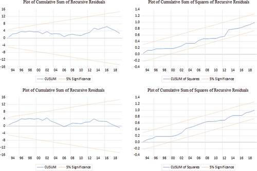
Figure 3. Plots of cumulative sums of recursive residuals and cumulative sums squares of recursive residuals: consumption model.

The straight lines indicate the critical bounds at 5% significance level.

Source: Authors’ estimations using EViews.

We also conducted diagnostic tests, the results of which are presented in Table 8. Based on these results, none of our model residuals had notable serial correlation, heteroskedasticity and non-normality. These results are in addition to the regression diagnostics that are reported in the lower panels of Tables 5 and 7. The measures reported therein indicate plausible goodness-of-fit and performance in respect of the estimated models. The final step in our empirical analysis is to assess how the impulse response functions compare with the ARDL results, and if they shed more light on the nature of the interactions involved.

Table 8. Diagnostic tests.

Test		test-statistic	p-value
	Investment model (1)
Serial Correlation LM Test:	Obs*R-squared	0.076	0.963
Heteroskedasticity Test:	Obs*R-squared	8.257	0.690
Normality Test:	Jarque-Bera	0.938	0.626
	Investment model (2)
Serial Correlation LM Test:	Obs*R-squared	0.561	0.755
Heteroskedasticity Test:	Obs*R-squared	8.029	0.711
Normality Test:	Jarque-Bera	1.620	0.445
	Consumption model
Serial Correlation LM Test:	Obs*R-squared	1.175	0.556
Heteroskedasticity Test:	Obs*R-squared	12.028	0.525
Normality Test:	Jarque-Bera	0.483	0.785

The serial correlation test results are based on the Breusch-Godfrey Serial Correlation LM (Lagrange Multiplier) Test under the null hypothesis of no serial correlation at up to 2 lags. The heteroskedasticity results are based on the Breusch-Pagan-Godfrey Test under the null hypothesis of homoskedasticity. The test-statistics follow a Chi-square distribution.

Source: Authors’ estimations using EViews.

4.2. Impulse response functions

Figures 4 through 6 display the plots of the IRFs that we estimated using the local projections method. In each plot, the response is shown by a solid line. The vertical axis shows the percentage point change in the response variable after a positive unit shock to another variable within the model. In the horizontal axis, we have the forecast horizons over which the response occurs (12 horizons in our case). Finally, the shaded areas represent 95% confidence intervals based on Newey-West heteroskedasticity and autocorrelation corrected (and finite-sample adjusted) standard errors. Since we had a small sample of annual time series, we estimated all the responses with one lag.

Figure 4. Responses of investment (linv), consumption (lcons) and real GDP (lgdp) to unit shocks to credit growth (lcred), interest rates (lintr), house prices (lhpi), stock prices (lspi) and exchange rates (lexr).

Source: Authors’ estimations using R.

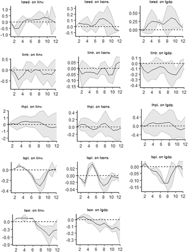
4.2.1. Unit shock to credit (lcred)

We begin with the responses (in Figure 4) of real variables to a unit shock in credit growth. We found that investment (linv) responds negatively to an increase in the stock of credit, on impact, but turns positive after several periods. Contrary to earlier findings, the current result suggests that an increase in the debt burden raises the cash-flow commitments to creditors, which constraints further investment (Fazzari, Ferri, and Greenberg 2008).

The reaction of consumption (lcons) to credit growth is positive in the immediate period but declines over several periods before it rises strongly. This is in line with the cycles proposed by Kapeller and Schütz (2014) which suggest that when outstanding debt reaches high levels and the solvency of borrowers worsens, lenders reduce credit supply. Consequently, consumers are forced to pay off their past debt and consolidate before another debt-financed consumption boom begins.

We can also note from Figure 4 that although the response of GDP (lgdp) to credit growth is negative on impact, it turns positive after two periods and remains as such for subsequent periods. The positive impact of credit reflects the importance of external finance in funding real economic activity.

4.2.2. Unit shock to interest rates (lintr)

Contrary to the ARDL results, we observed a negative response of investment to interest rates. The response fluctuates within the negative region for the duration of the forecast horizon. As we stated previously, a rise in interest rates translates into higher costs of finance and higher interest expenses on existing debt which, in turn, reduces available cash-flows that can be spent on investment.

Similarly, we note that the effect of interest rates on consumption is negative for most of the forecast horizon. This outcome is consistent with our earlier results. Furthermore, we also observe that, by constraining the components of demand, the tightening of interest rates also impacts negatively on GDP.

4.2.3. Unit shock to house prices (lhpi)

The positive reaction of investment to a rise in house prices indicates that the firms that invest in the real-estate sector are inclined to build when property values increase. The delayed response also reflects the fact that construction, as many other real investments, takes time to plan and implement (Bernanke, Gertler, and Gilchrist 1999). We see a similar delayed positive response from GDP which underscores the importance of property values for galvanising investment in the real-estate sector, which appears to have a positive spillover effect on the overall GDP.

The response of consumption is positive on impact but also evidently cyclical as the response to credit. The biggest effect of housing wealth on consumption is through its collateral value which enables house-owning consumers to access collateralised debt (Aoki, Proudman, and Vlieghe 2004). As such, credit growth may move somewhat closely with house price fluctuations (Ryoo 2016). This means that homeowners can borrow more when collateral values rise and less so when house values decline.

4.2.4. Unit shock to stock prices (lspi)

The response of investment to stock prices is a short-lasting one that turns negative after some time. If the claims on the deterring effect of shareholder value orientation on investment are anything to go by, this marginal response suggests that share prices are more important to the shareholders than to investment by the firm (Stockhammer 2005). We see a very similar picture from the GDP reaction to stock prices, which reiterates the very mild role that share prices play in stimulating growth. For consumption, the reaction is negative on impact. This consumption response confirms that financial wealth is generally possessed by economic agents with low consumption propensities, including firms.

4.2.5. Unit shock to the exchange rate (lexr)

The responses of investment and GDP to exchange rate shocks appear to be almost identical. The effects are positive but become negative after several horizons. Moreover, the negative reactions are larger than the earlier positive reactions, which implies that, despite the presence of the financial channel, the effect of exchange rates on trade is much more potent for economic activity in the South African economy. This finding somewhat challenges the existing evidence that the financial channel may cancel out the trade channel in emerging market economies (e.g. Kearns and Patel 2016). We, next, discuss the responses to unit increases in the distributional variables. These are exhibited in Figure 5.

Figure 5. Responses of investment (linv), consumption (lcons) and real GDP (lgdp) to unit shocks to the wage share (lws), profit share (lps) and income inequality (lincome10).

Source: Authors’ estimations using R.

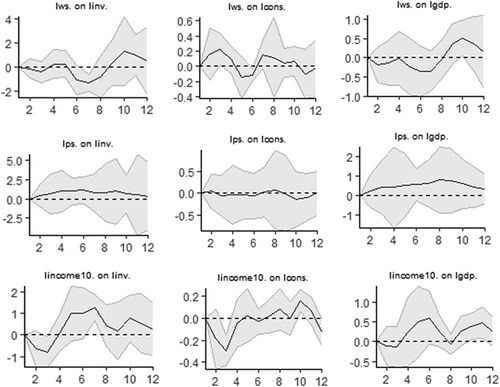
4.2.6. Unit shocks to the wage share (lws), profit share (lps) and income inequality (lincome10)

4.2.6.1. Consumption

Let us start with consumption responses to distributional shocks. Figure 5 shows that consumption reacts quite positively to an increase in the wage share and very mildly to the profit share. This is consistent with the ARDL results. Nonetheless, consumption out of labour income shows a cyclical response as it gets subdued after several horizons before it picks up again. Relatedly, the reaction to a shock to income inequality shows that consumption declines on impact and only recovers after several periods.

4.2.6.2. Investment

The response of investment to an increase in the wage share is negative for most of the forecast horizons. This is supportive of Fazzari, Ferri, and Greenberg’s (2008) proposition that a higher wage share reduces the internal funds that the firm would otherwise spend on investment. Moreover, the reaction to the profit share increase is mostly positive, which reiterates the importance of cash flows in alleviating financing constraints.

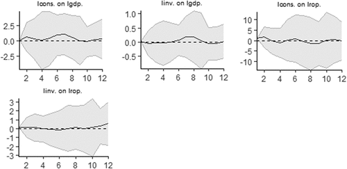
Finally, the immediate response of investment to a rise in income inequality is negative. This result shows that inequality is demand-reducing, on the one hand, and on the other hand, it challenges the notion that a rise in income inequality should raise aggregate savings, and thereby make more funds available for the productive sectors.

4.2.6.3. GDP

Regarding GDP, we note that a rise in income inequality elicits a negative reaction. This result shows that, by depressing demand, a rise inequality reduces overall growth. Interestingly, we also found that GDP responds quite positively to the growth of the profit share and negatively to the wage share. This implies that while labour income is important for consumption demand, economic growth is mostly led by profitability. Incidentally, the importance of aggregate demand for profitability that we alluded to earlier can be attested to by the immediate positive responses of the rate of profit (lrop) to increases in consumption and investment (see Figure 6).

Figure 6. Responses of real GDP (lgdp) to consumption (lcons) and investment (linv), and responses of rate of profit (lrop) to consumption (lcons) and investment (linv).

Source: Authors’ estimations using R.

Finally, we also note from Figure 6 that GDP responds positively to investment growth with a delay. We could attribute this sort of reaction to the time it takes to plan and get capital projects into operation. Consumption, on the other hand, elicits growth sooner rather than later.

In the final analysis, our GDP impulse response results suggest that, at least domestically and in the short-run cycle, the South African demand and/or growth regime might be of a character that Kapeller and Schütz (2015) described as a debt-financed-consumption-driven, profit-led regime. However, it is crucial to note that the local projection (LP) estimations did not account for the cointegration uncovered by the ARDL analysis, which may limit the accuracy of the IRF results (and the compatibility of the ARDL and LP methods). Therefore, the IRF findings should be approached with caution, as they may not fully capture the underlying relationships between the variables. Having concluded our empirical analysis, the next section summarises our key findings and concludes the paper.

5. Summary and conclusion

The aim of the study was to examine the impact of financial and distributional factors on demand and growth in the South African economy. Our results showed that the key financial factors influencing real activity are credit, interest rates, housing wealth, and exchange rates. In contrast, stock prices play a very mild role in influencing demand. The financial channel of exchange rates effectively influences investment demand, while the trade channel might have been more potent with respect to GDP. Moreover, our results indicated that distributional factors play a crucial role in influencing aggregate demand. Specifically, an increase in the wage share has a positive impact on consumer demand but a negative impact on investment and GDP. In comparison, the profit share exerts a positive effect on investment and GDP, but a moderate effect on consumption.

The key distributional variable in the study was income inequality (top 10% income share). We found that the rise in income inequality has had a significant suppressing impact on demand and overall growth. In conclusion, we recommend that any policy framework that the South African policymakers devise to galvanise economic growth should tackle the problem of inequality head-on.

Disclosure statement

No potential conflict of interest was reported by the author(s).

Data availability statement

The various data associated with this paper can be found in the South African central bank (SARB) website, the Organisation for Economic Cooperation and Development and the International Financial Statistics databases, the Word Inequality Database, and the World Profitability Dashboard.

Additional information

Funding

The work was supported by the National Research Foundation .

Notes

1. The survey and income tax data-based literature also place the increasing share of zero-wage individuals, as well as high unemployment, behind the growth of income inequality (Hundenborn, Woolard, and Jellema 2019).

2. This approach has some semblance of the Bhaduri and Marglin (1990) framework, which has spurred a corpus of empirical studies that investigate whether demand and growth regimes in various economies are wage-led or profit-led (e.g. Hein and Vogel 2008; Stockhammer and Wildauer 2016).

3. The adjustment is done using this formula: WS = (1 – GCONS)*WS^p + GCONS*WS^G => WS^p = (WS – GCONS)/(1-GCONS), where WS is the total wage share, GCONS is government consumption, WS^G is the public sector wage share, and WS^p is the private sector wage share (Gouzoulis, Constantine, and Ajefu 2021; Stockhammer 2017).

4. Credit to the anonymous reviewer who alerted us to this important point.

5. Blecker (2016) highlights the possibility of not capturing other insightful cyclical dynamic interactions when a separate-equations approach is adopted. Hence, we complementarily used a system-of-equations approach.

6. Short-term rates became a core instrument of South African monetary policy only from the late 1990s, more than a decade after the period used in this study begins.

Appendix

Table A1. Data description and sources.

Variable	Measure/indicator	Source of data
Real Gross Domestic Product (GDP)	GDP at market prices (constant prices-2015, seasonally adjusted, Rand millions)	South African Reserve Bank
Investment (INV)	Gross fixed capital formation (constant prices-2015, seasonally adjusted) – divided by real GDP by the authors	SARB
Consumption (CONS)	Final consumption expenditure by households (constant prices-2015, seasonally adjusted) – divided by real GDP by the authors	SARB
Credit (CRED)	Total credit extended to the private sector by monetary financial institutions – divided by real GDP by the authors	SARB
House prices (HPI)	Real house price indices	OECD database
Stock prices (SPI)	Real share price indices	OECD database
Exchange rate (EXR)	Nominal effective exchange rate against the most important currencies (Index, 2015 = 100)	SARB
Long-term interest rates (INTR)	Long-term government bond related interest rates	International Financial Statistics (IMF) database
Top 10% income share (INCOME10)	Top 10% income share of pre-tax national income	World Inequality Database
Adjusted wage share (WS)	Compensation of employees to GDP at factor cost	SARB
Profit share (PS)	Country-level profit shares, (net profit income/net output)	World Profitability Dashboard (Basu et al. 2022)
Rate of profit (ROP)	Country-level profit rates, (net profit income/capital stock)	World Profitability Dashboard (Basu et al. 2022)

SARB – South African Reserve Bank; OECD – Organisation for Economic Cooperation and Development; IMF – International Monetary Fund.

Table B1. Summary of descriptive statistics.

Variable	Mean	Maximum	Minimum	Std. Dev.	Obs.
INV	15.290	19.786	11.393	2.525	40
CONS	58.683	65.718	48.893	4.661	40
GDP	3092441.	4583667.	2032312.	887921.5	40
CRED	29.487	84.432	1.459	26.201	40
HPI	81.520	120.464	51.943	22.281	40
SPI	33.368	108.757	1.975	35.843	40
EXR	399.537	1490.032	89.269	403.571	40
INTR	12.059	16.901	7.722	3.330	40
INCOME10	0.545	0.650	0.460	0.0729	40
WS	43.636	51.941	37.334	3.863	40
PS	29.179	36.867	20.652	4.969	40
ROP	11.335	16.123	6.897	2.616	40

Sample: 1980–2019. All data in levels (i.e. not in log or differenced form). Obs.- number of observations. Std. Dev.-standard deviation. INV-investment, CONS-consumption, GDP-real GDP in market prices, CRED- domestic credit to private sector, HPI-house price index, SPI-stock price index, EXR-exchange rates, INTR-interest rates, INCOME10-top10% income share, WS- private wage share, PS-profit share, & ROP-rate of profit.

Source: Authors’ estimations using EViews.

References

- Aoki, K., J. Proudman, and G. Vlieghe. 2004. “House Prices, Consumption, and Monetary Policy: A Financial Accelerator Approach.” Journal of Financial Intermediation 13 (4): 414–435. https://doi.org/10.1016/j.jfi.2004.06.003.
- Ashman, Sam, Seeraj Mohamed, and Susan Newman. 2013. “The Financialization of the South African Economy and Its Impact on Economic Growth and Employment.” UNDESA Discussion Paper. New York, NY: United Nations Department of Economic and Social Affairs. https://uwe-repository.worktribe.com/index.php/preview/936665/Susan_retreat_UNDESA.pdf.
- Bassier, Ihsaan., and Ingrid Woolard. 2021. “Exclusive Growth? Rapidly Increasing Top Incomes Amid Low National Growth in South Africa.” South African Journal of Economics 89 (2): 246–273. https://doi.org/10.1111/saje.12274.
- Basu, Deepankar, Julio Huato, Jesus L. Jauregui, and Evan Wasner. 2022. “World Profit Rates, 1960–2019.” Review of Political Economy: 1–16. https://doi.org/10.1080/09538259.2022.2140007.
- Berg, Andrew G., and Jonathan D. Ostry. 2017. “Inequality and Unsustainable Growth: Two Sides of the Same Coin?” IMF Economic Review 65 (4): 792–815. https://doi.org/10.1057/s41308-017-0030-8.
- Bernanke, Ben S., and Mark Gertler. 1995. “Inside the Black Box: The Credit Channel of Monetary Policy Transmission.” Journal of Economic Perspectives 9 (4): 27–48. https://doi.org/10.1257/jep.9.4.27.
- Bernanke, Ben S., Mark Gertler, and Simon Gilchrist. 1999. “The Financial Accelerator in a Quantitative Business Cycle Framework.” In Handbook of Macroeconomics, edited by John B. Taylor and Michael Woodford, 1341–1393. Vol. 1. Amsterdam, NL: Elsevier B.V. https://doi.org/10.1016/S1574-0048(99)10034-X.
- Bernanke, B., M. Gertler, and S. Gilchrist. 1996. “The Financial Accelerator and the Flight to Quality.” The Review of Economics and Statistics 78 (1): 1–15. https://doi.org/10.2307/2109844.
- Bhaduri, A., and S. Marglin. 1990. “Unemployment and the Real Wage: The Economic Basis for Contesting Political Ideologies.” Cambridge Journal of Economics 14 (4): 375–393. https://doi.org/10.1093/oxfordjournals.cje.a035141.
- Blecker, Robert A. 2002. “Distribution, Demand and Growth in Neo-Kaleckian Macro-Models.” In The Economics of Demand-Led Growth: Challenging the Supply-Side Vision of the Long Run, edited by Mark Setterfield, 129–152. Northampton, MA: Edward Elgar Publishing Ltd.
- Blecker, Robert A. 2016. “Wage-Led versus Profit-Led Demand Regimes: The Long and the Short of it.” Review of Keynesian Economics 4 (4): 373–390. https://doi.org/10.4337/roke.2016.04.02.
- Borio, Claudio. 2014. “The Financial Cycle and Macroeconomics: What Have We Learnt?” Journal of Banking and Finance 45:82–198. https://doi.org/10.1016/j.jbankfin.2013.07.031.
- Carvalho, Laura., and Armon Rezai. 2016. “Personal Income Inequality and Aggregate Demand.” Cambridge Journal of Economics 40 (2): 491–505. https://doi.org/10.1093/cje/beu085.
- Chirinko, R. S., S. M. Fazzari, and A. P. Meyer. 1999. “How Responsive is Business Capital Formation to Its User Cost? An Exploration with Micro Data.” Journal of Public Economics 74 (1): 53–80. https://doi.org/10.1016/S0047-2727(99)00024-9.
- Chirinko, R. S., S. M. Fazzari, and A. P. Meyer. 2011. “A New Approach to Estimating Production Function Parameters: The Elusive Capital–Labor Substitution Elasticity.” Journal of Business & Economic Statistics 29 (4): 587–594. https://doi.org/10.1198/jbes.2011.08119.
- Correia, C. 2015. Financial Management. Cape Town, RSA: Juta & Company Ltd.
- Driver, Ciaran, and Laurence Harris. 2021. “Investment in South Africa.” In The Oxford Handbook of the South African Economy, edited by Arkebe Oqubay, Fiona Tregenna, and Imraan Valodia, 913–935. Oxford, UK: Oxford University Press.
- Du Plessis, Stan, and Ben, Smit. 2009. “Accounting for South Africa’s Growth Revival After 1994.” In South African Economic Policy Under Democracy, edited by Janine Aron, Brian Kahn, and Geeta Kingdon, 28–57. Oxford, UK: Oxford University Press.
- Dutt, Amitava K. 2006. “Maturity, Stagnation and Consumer Debt: A Steindlian Approach.” Metroeconomica 57 (3): 339–364. https://doi.org/10.1111/j.1467-999X.2006.00246.x.
- Elliott, G., T. J. Rothenberg, and J. H. Stock. 1996. “Efficient Tests for an Autoregressive Unit Root.” Econometrica 64 (4): 813–836. https://doi.org/10.2307/2171846.
- Fazzari, S., P. Ferri, and E. Greenberg. 2008. “Cash Flow, Investment, and Keynes–Minsky Cycles.” Journal of Economic Behavior and Organization 65 (3–4): 555–572. https://doi.org/10.1016/j.jebo.2005.11.007.
- Finn, Arden, and Murray Leibbrandt. 2018. “The Evolution and Determination of Earnings Inequality in Post-Apartheid South Africa.” UNU-WIDER Working Paper 2018/83. Helsinki, Finland: United Nations University World Institute for Development Economics Research. https://doi.org/10.35188/UNU-WIDER/2018/525-1.
- Gouzoulis, G., C. Constantine, and J. Ajefu. 2021. “Economic and Political Determinants of the South African Labour Share, 1971–2019.” Economic and Industrial Democracy 44 (1): 184–207. https://doi.org/10.1177/0143831X211063230.
- Hawkins, Penelope. 2021. “Banking and Finance in South Africa.” In The Oxford Handbook of the South African Economy, edited by Arkebe Oqubay, Fiona Tregenna, and Imraan Valodia, 992–1013. Oxford, UK: Oxford University Press.
- Hein, Eckhard., and Lena Vogel. 2008. “Distribution and Growth Reconsidered: Empirical Results for Six OECD Countries.” Cambridge Journal of Economics 32 (3): 479–511. https://doi.org/10.1093/cje/bem047.
- Hundenborn, Janina, Murray Leibbrandt, and Ingrid Woolard. 2018. “Drivers of Inequality in South Africa.” UNU-WIDER Working Paper 2018/162. Helsinki, Finland: United Nations University World Institute for Development Economics Research. https://doi.org/10.35188/UNU-WIDER/2018/604-3.
- Hundenborn, Janina, Ingrid Woolard, and Jon Jellema. 2019. “The Effect of Top Incomes on Inequality in South Africa.” International Tax and Public Finance 26 (5): 1018–1047. https://doi.org/10.1007/s10797-018-9529-9.
- Jordà, Òscar. 2005. “Estimation and Inference of Impulse Responses by Local Projections.” The American Economic Review 95 (1): 161–182. https://doi.org/10.1257/0002828053828518.
- Kalecki, M. 1954. Theory of Economic Dynamics. London, UK: Routledge.
- Kapeller, Jakob., and Bernhard Schütz. 2014. “Debt, Boom, Bust: A Theory of Minsky-Veblen Cycles.” Journal of Post Keynesian Economics 36 (4): 781–814. https://doi.org/10.2753/PKE0160-3477360409.
- Kapeller, Jakob., and Bernhard Schütz. 2015. “Conspicuous Consumption, Inequality and Debt: The Nature of Consumption-Driven Profit-Led Regimes.” Metroeconomica 66 (1): 51–70. https://doi.org/10.1111/meca.12061.
- Kearns, Jonathan., and Nikhil Patel. 2016. “Does the Financial Channel of Exchange Rates Offset the Trade Channel?” BIS Quarterly Review 2016:95–113. https://www.bis.org/publ/qtrpdf/r_qt1612i.pdf.
- Kohler, Karsten. 2019. “Exchange Rate Dynamics, Balance Sheet Effects, and Capital Flows. A Minskyan Model of Emerging Market Boom-Bust Cycles.” Structural Change and Economic Dynamics 51:270–283. https://doi.org/10.1016/j.strueco.2019.09.006.
- Kohler, Karsten., and Engelbert Stockhammer. 2022. “Flexible Exchange Rates in Emerging Markets: Shock Absorbers or Drivers of Endogenous Cycles?” Industrial and Corporate Change 32 (2): 551–572. https://doi.org/10.1093/icc/dtac036.
- Kumhof, M., R. Rancière, and P. Winant. 2015. “Inequality, Leverage, and Crises.” The American Economic Review 105 (3): 1217–1245. https://doi.org/10.1257/aer.20110683.
- Leibbrandt, M., A. Finn, and I. Woolard. 2012. “Describing and Decomposing Post-Apartheid Income Inequality in South Africa.” Development Southern Africa 29 (1): 19–34. https://doi.org/10.1080/0376835X.2012.645639.
- Leibbrandt, Murray, Vimal Ranchhod, and Pippa Green. 2021. “The Top End, Labour Markets, Fiscal Redistribution, and the Persistence of Very High Inequality.” In Inequality in the Developing World, edited by Carlos Gradín, Murray Leibbrandt, and Finn Tarp, 205–229. United Nations University World Institute for Development Economics Research (UNU-WIDER). Oxford, UK: Oxford University Press.
- Marglin, Stephen, and Amit. Bhaduri. 1991. “Profit Squeeze and Keynesian Theory.” In Nicholas Kaldor and Mainstream Economics Confrontation or Convergence? edited by Edward J. Nell and Willi Semmler, 123–163. New York, NY: Palgrave Macmillan.
- Minsky, H. P. 1975. John Maynard Keynes. New York, NY: Columbia University Press.
- Minsky, H. P. [1982]2016. Can “It” Happen Again? Essays on Instability and Finance. New York, NY: Routledge.
- Minsky, H. P. 1986. Stabilizing an Unstable Economy. New Haven, CT: Yale University Press.
- Narayan, Paresh K. 2005. “The Saving and Investment Nexus for China: Evidence from Cointegration Tests.” Applied Economics 37 (17): 1979–1990. https://doi.org/10.1080/00036840500278103.
- Palley, Thomas I. 1994. “Debt, Aggregate Demand, and the Business Cycle: An Analysis in the Spirit of Kaldor and Minsky.” Journal of Post Keynesian Economics 16 (3): 371–390. https://doi.org/10.1080/01603477.1994.11489991.
- Palley, Thomas I. 2017. “Wage- Vs. Profit-Led Growth: The Role of the Distribution of Wages in Determining Regime Character.” Cambridge Journal of Economics 41 (1): 49–61. https://doi.org/10.1093/cje/bew004.
- Perron, Pierre. 1989. “The Great Crash, the Oil Price Shock, and the Unit Root Hypothesis.” Econometrica 57 (6): 1361–1401. https://doi.org/10.2307/1913712.
- Perron, Pierre. 1997. “Further Evidence on Breaking Trend Functions in Macroeconomic Variables.” Journal of Econometrics 80 (2): 355–385. https://doi.org/10.1016/S0304-4076(97)00049-3.
- Pesaran, M. H., K. Shin, and R. J. Smith. 2001. “Bounds Testing Approaches to the Analysis of Level Relationships.” Journal of Applied Econometrics 16 (3): 289–326. https://doi.org/10.1002/jae.616.
- Rey, Hélène. 2016. “International Channels of Transmission of Monetary Policy and the Mundellian Trilemma.” IMF Economic Review 64 (1): 6–35. https://doi.org/10.1057/imfer.2016.4.
- Ryoo, Soon. 2010. “Long Waves and Short Cycles in a Model of Endogenous Financial Fragility.” Journal of Economic Behavior and Organization 74 (3): 163–186. https://doi.org/10.1016/j.jebo.2010.03.015.
- Ryoo, Soon. 2013. “Minsky Cycles in Keynesian Models of Growth and Distribution.” Review of Keynesian Economics 1 (1): 37–60. https://doi.org/10.4337/roke.2013.01.03.
- Ryoo, Soon. 2016. “Household Debt and Housing Bubbles: A Minskian Approach to Boom-Bust Cycles.” Journal of Evolutionary Economics 26 (5): 971–1006. https://doi.org/10.1007/s00191-016-0473-5.
- Ryoo, Soon., and Yun K. Kim. 2014. “Income Distribution, Consumer Debt and Keeping Up with the Joneses.” Metroeconomica 65 (4): 585–618. https://doi.org/10.1111/meca.12052.
- StatsSA (Statistics South Africa). 2019. Inequality Trends in South Africa: A Multidimensional Diagnostic of Inequality. Pretoria, RSA: Statistics South Africa.
- Stockhammer, Engelbert. 2005. “Shareholder Value Orientation and the Investment-Profit Puzzle.” Journal of Post Keynesian Economics 28 (2): 193–215. https://doi.org/10.2753/PKE0160-3477280203.
- Stockhammer, Engelbert. 2015. “Rising Inequality as a Cause of the Present Crisis.” Cambridge Journal of Economics 39 (3): 935–958. https://doi.org/10.1093/cje/bet052.
- Stockhammer, Engelbert. 2017. “Determinants of the Wage Share: A Panel Analysis of Advanced and Developing Economies.” British Journal of Industrial Relations 55 (1): 3–33. https://doi.org/10.1111/bjir.12165.
- Stockhammer, Engelbert., and Rafael Wildauer. 2016. “Debt-Driven Growth? Wealth, Distribution and Demand in OECD Countries.” Cambridge Journal of Economics 40 (6): 1609–1634. https://doi.org/10.1093/cje/bev070.
- Terreblanche, S. 2002. A History of Inequality in South Africa 1652–2002. Pietermaritzburg, RSA: University of KwaZulu-Natal Press.
- Wittenberg, Martin. 2017. “Wages and Wage Inequality in South Africa 1994–2011: Part 2 – Inequality Measurement and Trends.” South African Journal of Economics 85 (2): 298–318. https://doi.org/10.1111/saje.12147.