Temporal changes in size distributions of the Southern Ocean diatom Fragilariopsis kerguelensis through high-throughput microscopy of sediment trap samples

Abstract

Some aspects of the life cycle of the Southern Ocean diatom Fragilariopsis kerguelensis have been investigated previously, but many of its details have not been surveyed in nature. We investigated material from a two-year sediment trap time series by high-throughput imaging and image analysis, looking for morphometric signals of life cycle stages. Valve length distributions appeared close to unimodal but positively (right-) skewed. Size cohorts resulting from synchronized sexual reproduction events were not clearly distinguishable. Nevertheless, based on changes in valve length distributions, we found three general seasonal phases. These corresponded to periods of proliferation (with higher proportions of smaller cells during late spring/early summer), cessation of growth (relative loss of smaller cells during late summer/early autumn), and overwintering (little change in size distributions, with an increased proportion of large cells). We discuss possible causes of these signals, and their relevance to growth, sexual activity and adaption to environmental conditions, such as grazing pressures and the need for an overwintering strategy.

Keywords:

• morphometry
• phytoplankton
• SHERPA
• slide scanner
• valve size distribution

Abbreviations: ACC: Antarctic Circumpolar Current; APF: Antarctic Polar Front; EIFEX: European Iron Fertilization Experiment; HNLC: high-nutrient low-chlorophyll; PFZ: Polar Frontal Zone; RI: ranking index; RFI: relative frequency of valves within the initial cell size range

Introduction

The pelagic pennate diatom Fragilariopsis kerguelensis (O’Meara) Hustedt is endemic to the Southern Ocean (Hart 1942, Zielinski & Gersonde 1997, Cortese & Gersonde 2008). The species usually occurs in chains of up to dozens of cells throughout the Southern Ocean, and the Polar Frontal Zone (PFZ) of the Antarctic Circumpolar Current (ACC) is considered to be its optimal habitat (Zielinski & Gersonde 1997, Cortese & Gersonde 2007, Pinkernell & Beszteri 2014). A major fraction of the silicic acid brought to the Southern Ocean surface waters by the global overturning thermohaline circulation is exported to the sediment by a handful of strongly silicified diatom species, of which F. kerguelensis is the best studied (Assmy et al. 2013). Indeed, frustules of F. kerguelensis are the main contributor to a band of silica-rich sediments that encircle Antarctica, known as the ‘diatom ooze belt’. This diatom ooze belt accounts for approximately one-third of the global biogenic silica accumulation (Tréguer & De La Rocha 2013, Tréguer 2014), forming the largest sink for silica in the global ocean. High abundances of F. kerguelensis in Southern Ocean sediments are regarded as an indication of low-carbon high-silica exporting regimes (Smetacek et al. 2004, Abelmann et al. 2006, Assmy et al. 2013). For these and other reasons, the species has generated interest in several fields of research, spanning biological oceanography (DeBaar et al. 1997, Hoffmann et al. 2007, Assmy et al. 2013), biogeography (Pinkernell & Beszteri 2014), paleoceanography (Cortese & Gersonde 2007, 2008, Esper et al. 2010, Cortese et al. 2012, Shukla et al. 2013, Shukla & Crosta 2017, Kloster et al. 2018, Shukla & Romero 2018), ecophysiology (Timmermans & Van Der Wagt 2010, Trimborn et al. 2013, 2014, Beszteri et al. 2018b), and biomechanics (Hamm et al. 2003, Wilken et al. 2011).

The life cycle of F. kerguelensis has been investigated previously. Assmy et al. (2006) observed auxosporulation in the field during a large scale iron fertilization experiment in the PFZ. They gave a morphological description of the auxospores of the species, and estimated their relative abundances as between 0.03% and 0.4% of the population. Since more auxospores were observed where higher absolute abundances of the species occurred, it was hypothesized that sexualization preceding auxosporulation might be density dependent. Based on the fact that no more than one gametangium was found connected to any of the auxospores, it was suggested that auxospore production might have been preceded either by ‘type II’ fertilization giving rise to one auxospore per pairing (Geitler 1973), or possibly by self-fertilization, although this was considered less likely, based on the lack of auxosporulation in clonal cultures (Assmy et al. 2006). Fuchs et al. (2013) extended these results by observation of laboratory crosses between clonal cultures. They found a dioecious pattern of compatibility among the clones studied and described the process of sexual induction as starting with the disintegration of chains, followed by subsequent gametogenesis and auxospore production, although fertilization was not directly observed.

Diatoms have a unique life cycle generally consisting of size reduction during vegetative growth, and size restoration by auxospore production, mostly following sexual reproduction (Round et al. 1990, Edlund & Stoermer 1997). Accordingly, the cell size below which sexuality can be induced, as well as the largest possible cell size for the species, are the two cardinal points of the life cycle. Initial estimates for the former can be derived from the size of gametangia, for the latter from auxospores or initial cells. In the field, Assmy et al. (2006) observed gametangia attached to auxospores to be between 10 and 31 µm long, and auxospores containing initial cells between 76 and 90 µm. Under laboratory conditions, Fuchs et al. (2013) found gametangial thecae between 6.9 and 26.1 µm long and initial cells between 78.4 and 100.8 µm long. Following population size distributions over time has in several cases enabled individual cohorts to be followed through size decrease or auxosporulation events, thereby providing valuable insights into the life history of these diatoms (Stoermer et al. 1989, Jewson 1992a, 1992b, D’Alelio et al. 2010, Bishop & Spaulding 2017). Moving beyond visual interpretation of size distribution profiles, Card & Carra (2013) decomposed size distributions into component binomial expansions, whereas Schwarz et al. (2009) and Bishop & Spaulding (2017) applied Gaussian mixture modelling for the same purpose, and Schwarz et al. (2009) and D’Alelio et al. (2010) developed models to follow the size reduction process in individual cohorts. It is not simple to obtain such information about a Southern Ocean diatom because their remote habitat is difficult to sample repeatedly over longer time periods. As an alternative, Cortese & Gersonde (2007) measured valve area distributions sampled over the course of a year by two moored sediments traps, but since their focus was not on the life cycle, they only presented average values for each time point sampled. The present study addresses this gap, by analyzing a size distribution time of F. kerguelensis obtained using sediment traps over the course of two consecutive years in the PFZ south of Australia.

Assessments of cell size distributions require large sample sizes if individual cohorts and, presumably rare, auxosporulation events are to be detected. For example, Crawford et al. (1997) determined the size of 1,000 valves per sample of Corethron criophilum Castracane, and D’Alelio et al. (2010) investigated Pseudo-nitzschia multistriata (H.Takano) H.Takano temporal size variations analyzing 200 cells per sample. Manually measuring such large numbers of specimens is tedious. To address this, the FlowCAM^® (Fluid Imaging Technologies, Inc., Scarborough, ME, USA) imaging flow cytometer was utilized to measure large numbers of diatom valves in an automated manner by Spaulding et al. (2012) and Bishop & Spaulding (2017). In this study, we present a different technological approach to the same challenge, using a combination of slide-scanning light microscopy and image analysis (Kloster et al. 2014, 2017), which can be considered a semi-automated variant of the more traditional, slide-based diatom analyses, and which we have successfully applied in other morphometric studies recently (Beszteri et al. 2018a, Kloster et al. 2018).

By characterizing a time series of valve length distributions using this semi-automated procedure, we wanted to gain insights into the annual progression of F. kerguelensis through different life cycle phases and into the timing of auxosporulation events.

Material and methods

We analysed material covering the period from November 2002 to October 2004 collected by a sediment trap at 800 m below the ocean surface which was moored near 54°S 140°E in ca. 2300 m water depth, close to the top of the Australia-Antarctica mid-ocean ridge. Further details of the sediment trap, sampling, and material processing are described in Rigual-Hernández et al. (2015). Importantly, collections at this site in previous years contained negligible lithogenic material (Trull et al. 2001a), and light transmissometry profiles (e.g., Bowie et al. 2011) suggest that resuspension of bottom sediments does not deliver material to this trap.

Oceanographic setting of the 54°S site

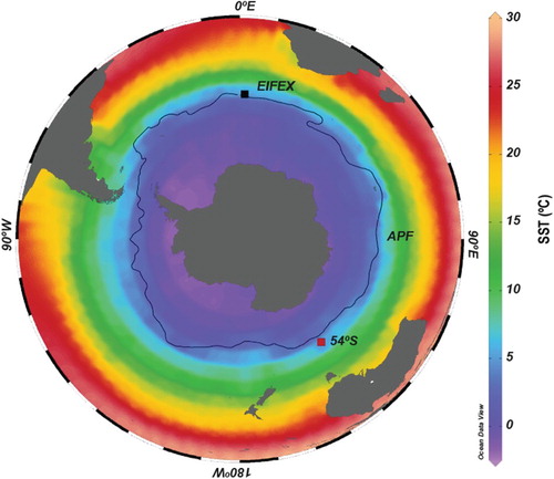
The sediment trap site (Fig. 1) is located within the central area of the PFZ, i.e., within the rapidly flowing ACC that lies between the Antarctic Polar Front (APF) and the Subantarctic Front (Trull et al. 2001a, Trull et al. 2001b, Rigual-Hernández et al. 2015). These waters are part of the canonical high-nutrient low-chlorophyll Southern Ocean habitat in which phytoplankton production is limited by iron availability and thus macro-nutrients are not fully consumed seasonally (e.g., Martin et al. 1990, Trull et al. 2001b). At the 54°S site the macro-nutrients nitrate and phosphate are abundant year-round, but the silicate required by diatoms to form their frustules becomes strongly depleted by late summer (Trull et al. 2001b, Bowie et al. 2011). Iron is re-supplied at low levels, primarily by deep winter mixing, and appears to be limiting to phytoplankton growth throughout the year (Bowie et al. 2009).

Fig. 1. Map of the Southern Ocean with annual sea surface temperatures (SST; World Ocean Atlas 2013, Locarnini et al. 2013) showing the location of the 54°S station and the site of the European Iron Fertilization Experiment (EIFEX). Black line represents the position of the APF after Orsi et al. (1995).

Chlorophyll-a and flux data

Chlorophyll-a concentration was derived from NASA’s Giovanni online data system. Flux data were obtained from Rigual-Hernández et al. (2015). We estimate that signals originating from the sediment trap material are delayed by ca. 2–6 weeks compared to the chlorophyll-a data, due to the time required for the material to reach the sediment trap at 800 m depth. Subsurface chlorophyll-a maxima do occur in PFZ waters in this region, but appear to be largely dormant and are thus unlikely to contribute strongly to population dynamics (Parslow et al. 2001).

Microscopy

Microscope slides were prepared as described by Rigual-Hernández et al. (2015). Microscopy and morphometric measurements were conducted using a Metafer automated slide scanner (MetaSystems Hard & Software GmbH, Altlussheim, Germany) and our diatom morphometry software SHERPA version 1.1c (Kloster et al. 2014), according to our previously described workflow (Kloster et al. 2017). Briefly, a rectangular area on each slide was scanned, in overlapping fields of view, with a Plan-NEOFLUAR 20× objective (Carl Zeiss AG, Oberkochen, Germany). These low-resolution images were compared by SHERPA to a template library of diverse outline shapes representing the genus Fragilariopsis Hustedt (see supplement ‘SHERPA settings’), to locate valves of interest in the captured area. Positions where valves were found were then revisited in the Metafer system using a high-resolution oil immersion objective (Plan-APOCHROMAT 63x/1.4, Carl Zeiss AG, Oberkochen, Germany). Each valve was captured in 20 different focal planes, and focus stacking was applied to generate an image with an enhanced depth of field. The enhanced images were then analysed with SHERPA for morphometric measurements. Contrasting the traditional manual approach, this semi-automated workflow requires each selected scanning area to be processed entirely to prevent introducing bias by SHERPA’s result ranking procedure. Accordingly, sampling numbers vary for different slides, depending on valve density and scanned area. Settings files used for SHERPA analyses of both the low and high-resolution images, as well as the relevant shape templates, are included in the supplementary material (see supplement ‘SHERPA settings’).

Because of the relatively low refractive index (1.56) of the NOA 61 mounting agent (Norland Products Inc., Cranbury, NJ, USA), imaging contrast was poorer than in Naphrax, causing a decreased accuracy in object segmentation and outline detection. To compensate for this shortcoming, increased manual intervention was necessary in SHERPA, for post-editing as well as reviewing segmentation results (see supplement ‘Modified SHERPA procedure’).

Data analysis

As a more quantitative approach to explore whether some distributions can be decomposed into individual cohorts, we modelled the observed valve length distributions for each sample as mixtures of one to six univariate normal distributions. These mixture models were fitted using an expectation maximization algorithm (Benaglia et al. 2009), in addition to the single-component normal distribution, to account for the possibility that only one cohort was present. The best-fitting model (number of cohorts) was determined as the one with the lowest Bayesian information criterion (see supplement ‘R scripts’).

To trace auxosporulation and size restitution events, the relative abundance of very large valves was determined. Fragilariopsis kerguelensis average valve length peaks beneath the APF in the Southern Ocean sediments (Cortese & Gersonde 2007). Close to the APF, in the Atlantic sector of the Southern Ocean (49°S 2°E), the only observation of F. kerguelensis sexual activity in its natural habitat was made by Assmy et al. (2006) during the European Iron Fertilization Experiment (EIFEX). Since our sampling site is also close to the APF, we assume that data on valve length from both sites should be comparable. For the EIFEX experiment, auxospores of F. kerguelensis containing initial thecae were reported to be at least 76 µm long. We assumed that valves longer than 75.5 µm originate either from initial cells or cells descended from them by only a few divisions, and refer to them as within the initial cell size range. These large cells were very rare, and their counts were strongly affected by the maximum ‘ranking index’ (RI) considered during manual checking of SHERPA results (please see supplement ‘Modified SHERPA procedure’ and Kloster et al. 2014, 2017 for further information). Accordingly, relative abundance calculated from counts utilizing different highest RIs might be underestimated (respective results are listed in supplement ‘Valves within the initial cell size range’). To compensate for this, they were searched for in an additional reviewing run, by examining high-resolution results of RI 0–6 for each slide, regardless of the maximum RI used for retrieving the valve length distribution. The corresponding counts were normalized to the amount of material suspension on the slide, the scanned slide area (approximated by the number of fields of view scanned at low magnification), the length of the sampling period for the corresponding cup of the sediment trap, and the F. kerguelensis flux rates (from Rigual-Hernández et al. 2015) to characterize the relative frequency of valves within the initial cell size range (RFI) in the population (see Equation (1)). These values use an arbitrary scale and are only comparable with each other. (1) $\mathit{\text{RFI}}=\frac{\left(\mathit{\text{number}}\mathit{\text{of}}\mathit{\text{valves}}\ge 75.5\text{μ}m\right)\cdot {10}^{12}}{\mathit{\text{amount}}\mathit{\text{of}}\mathit{\text{suspension}}\cdot \mathit{\text{nFOVs}}\cdot \mathit{\text{spl}}\cdot \mathit{\text{valve}}\mathit{\text{flux}}}$(1) with nFOVs = number of scanned fields of view, spl = sampling period length.

A rough estimation of the growth rate is possible for periods with an ongoing decrease in mean valve length, based on the length reduction per division and the average cell size decrease of the population, assuming that the average size decrease was caused only by vegetative proliferation: (2) $\begin{array}{r}\mathit{\text{est.}}\mathit{\text{growth}}\mathit{\text{rate}}=\frac{l_2-l_1}{(t_2-t_1)\cdot \mathit{\text{cell}}\mathit{\text{size}}\mathit{\text{decrease}}\cdot {\mathit{\text{divison}}}^{-1}}\end{array}$(2) with $l_1$, $l_2$ = mean valve length at time $t_1$, $t_2$

An estimate of 0.28 µm/division for the cell size decrease was assumed following Fuchs et al. (2013).

Of the morphometric parameters determined by SHERPA, we present the apical valve lengths and the variation in their distribution over time. Downstream analysis of counts and valve sizes was performed using scripts (see supplement ‘R scripts’) programmed in R (R Core Team 2015). Measurements of additional features, such as transapical length, valve area, costa distance and F (Fenner et al. 1976) or F* (Cortese & Gersonde 2007) are included in the supplementary material (see ‘Additional measurements’ for respective plots and ‘Data’ for the complete data set).

Results

In total, we measured ca. 29,000 F. kerguelensis valves from 43 slides, representing 41 different samples, covering the period from November 2002 to October 2004. For visual exploration, changes in F. kerguelensis valve length distribution throughout the two sampling years were plotted as histograms (Figs 2–3) and as violin plots (Figs 4–5). The size distributions were close to unimodal, positively (right-) skewed, and similar to the measurements reported by Crosta (2009) for sediment core material integrated over longer timescales. The quantitative exploration of size cohorts mostly showed 2–3 components for each time point (Figs 2–3 coloured density curves; note that curves appearing in the same colour at different time points do not necessarily correspond to the same cohort). The main peak in the distributions was mostly detected well by this approach, and in some cases a secondary peak, corresponding to the expectation for a larger sized, lower abundance cohort (see e.g., cup 2.19 from August 2004 in the left bottom of Fig. 3) was also detected. However, the Gaussian mixture modelling tended to converge towards different component compositions depending on starting values for some samples (e.g., cups 1.05, 1.19, 1.20, 2.01, 2.02, 2.12). The minor components are in most cases not clearly interpretable as distinct size cohorts, because they represented rather flat distributions of large sizes. To overcome the problem that post-initial valves are always rare and that their abundance might be underestimated using our standard counting scheme, we determined the relative frequency of ‘initial’ cells (RFI, see Equation (1) and Figs 4–5, h).

Fig. 2. Distributions of valve lengths and mixtures of univariate normal distributions for sampling year 2002/2003. Background colours red, green and blue depict phases 1, 2 and 3 explained in the text. Histograms show the distribution of measured valve lengths, the dashed curve their density estimate. Vertical dotted lines mark 31 µm, the size limit below which sexual reproduction can occur, and 75.5 µm, the minimal size of initial cells as reported by Assmy et al. (2006). Coloured curves depict the component normal distributions C1-Cn, the corresponding parameters are given in the graphs. Note that curves appearing in the same colour at different time points are not implied to correspond to the same cohort (colour online).

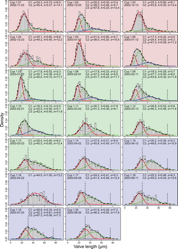
Fig. 3. Distributions of valve lengths and mixtures of univariate normal distributions for sampling year 2003/2004. Background colours red, green and blue depict phases 1, 2 and 3 explained in the text. Histograms show the distribution of measured valve lengths, the dashed curve their density estimate. Vertical dotted lines mark 31 µm, the size limit below which sexual reproduction can occur, and 75.5 µm, the minimal size of initial cells as reported by Assmy et al. (2006). Coloured curves depict the component normal distributions C1-Cn, the corresponding parameters are given in the graphs. Note that curves appearing in the same colour at different time points are not implied to correspond to the same cohort (colour online).

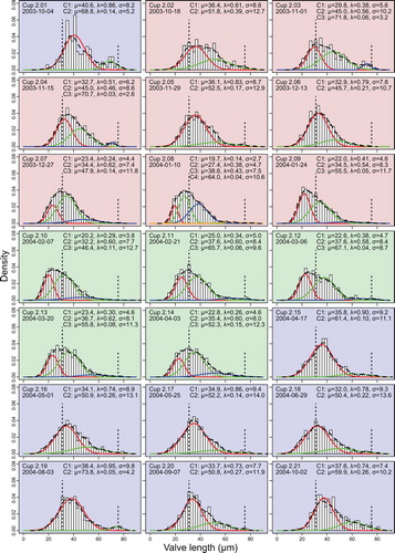
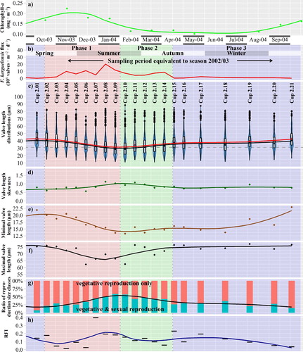
Fig. 4. Temporal variability during sampling year 2002/2003, x-axis refers to the middle day of sampling periods. (a) Chlorophyll-a concentration in the upper water column. (b–h) Sediment trap data from 800 m depth, for Fragilariopsis kerguelensis; depending on the sinking speed, the timeline is delayed by ca. 2–6 weeks compared to the chlorophyll data. Trend lines are derived by LOESS smoothing: (b) Valve flux. (c) Valve length. Blue violin plots depict the value distributions, box plots represent quartiles, red dots indicate the mean, black dots inside the boxplots the median. The dashed horizontal line depicts 31 µm, the size limit below which sexual reproduction can occur. (d) Seasonal changes in the valve length skewness. (e) Minimal valve length by 0.01 quantile. (f) Maximal valve length by 0.99 quantile. (g) Ratio of size fractions which are sexually inducible (that are capable of vegetative as well as sexual reproduction, with a valve length below 31 µm, highlighted in turquoise), respectively, capable of vegetative reproduction only (orange). (h) Relative frequency of valves within the initial cell size range (RFI), as an indicator for initial cells (colour online).

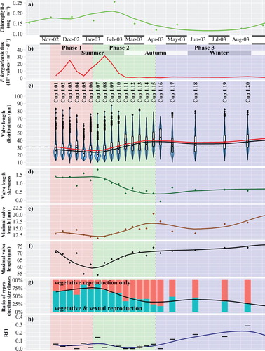
Fig. 5. Temporal variability during sampling year 2003/2004, x-axis refers to the middle day of sampling periods. (a) Chlorophyll-a concentration in the upper water column. (b–h) Sediment trap data from 800 m depth for Fragilariopsis kerguelensis; depending on the sinking speed, the timeline is delayed by ca. 2–6 weeks compared to the chlorophyll data. Trend lines are derived by LOESS smoothing: (b) Valve flux. (c) Valve length. Blue violin plots depict the value distributions, box plots represent quartiles, red dots indicate the mean, black dots inside the boxplots the median. The dashed horizontal line depicts 31 µm, the size limit below which sexual reproduction can occur. (d) Seasonal changes of the valve length skewness. (e) Minimal valve length by 0.01 quantile. (f) Maximal valve length by 0.99 quantile. (g) Ratio of size fractions which are sexually inducible (that are capable of vegetative as well as sexual reproduction, with a valve length below 31 µm, highlighted in turquoise), respectively, capable of vegetative reproduction only (orange). (h) Relative frequency of valves within the initial cell size range (RFI), as an indicator for initial cells (colour online).

Although the size distribution histograms show changes, clear shifts to the left in modes of the distribution, or of component distributions obtained with mixture modelling, could rarely be recognized. Such shifts would be expected to signal periods of vegetative growth accompanied by a reduction in the average size of the population. The clearest exception is the beginning of the growing season at the end of 2003 (histograms with red background in Fig. 3). Here, a relatively continuous shift of the main mode of the distribution towards smaller sizes can be observed between mid-October 2003 and late January 2004 (cups 2.02–2.09).

Given the lack of clearly separable size cohorts, we focused on changes in valve lengths illustrated by average, minimal and maximal values, as well as by distribution skewness and the proportion of the size classes of sexually inducible, not sexually inducible and initial cells (Figs 4–5). These exhibited a seasonal pattern which, in general, was similar for both sampling years, even though less pronounced for the second year. This pattern was characterized by three different phases:

• During phase 1 (late spring/early summer, highlighted by a red background in Figs 2–5), an accumulating proportion of short valves led to decreasing median valve lengths (see also supplement ‘Detail on valve lengths’) and increasing skewness. At the same time, minimal and maximal valve length decreased.

• During phase 2 (late summer/early autumn, highlighted by a green background in Figs 2–5) trends from phase 1 were inverted: loss of short valves led to increasing median valve lengths (see also supplement ‘Detail on valve lengths’) and decreasing skewness. At the same time, minimal and maximal valve size increased.

• During phase 3 (mid-autumn until mid-spring, highlighted by a blue background in Figs 2–5) only small changes were observable in valve length distributions. The populations contained the lowest proportion of sexually inducible cells, and minimal valve length increased during the second half of this phase.

Changes in the median valve length were also seen in the values for valve width (transapical axis length), valve area, costa distance and F or F*, although not all these morphometric characters would be considered as being related to size (see supplement ‘Additional measurements’).

Discussion

Vegetative reproduction

During phase 1, from mid-spring until mid-summer, the proportion of smaller cells increased, shifting both the median and minimum valve lengths to the left. This was probably caused by prevailing vegetative reproduction (also in line with increasing chlorophyll-a concentrations and species-specific valve fluxes, panels a and b of Figs 4–5), adding an increasing quantity of progressively smaller cells to the population. The parallel decreasing maximal valve length might indicate that the largest sized subpopulation was not replenished significantly by auxosporulation (discussed below).

Sexual reproduction

A synchronized sexual reproduction event is expected to produce signals in a time series of cell size distributions: The proportion of smaller, sexually inducible cells would suddenly drop due to gametogenesis, followed by the appearance of large cells within or close to the size range of initial cells. The above described vegetative growth during phase 1 led to an increasing proportion of valves in the sexually inducible size range. These provided up to about 80% (cup 1.07/late January 2003) in the first sampling year, and up to 60% (cup 2.09/late January 2004) in the second year (see Figs 4–5, c – portions below the dashed lines, respectively, g – turquoise bars), so that the majority of the population should have been inducible. Minimal valve length then decreased, along with increasing maximal length, which could indicate auxosporulation. Subsequently the decline in smaller cells continued for several months throughout phase 2 (cups 1.08–1.16: February–April. 2003, Fig. 2; and cups 2.10–2.15: February–April 2004, Fig. 3). This could possibly reflect death or removal of the smallest cell fraction not involved in sexual reproduction because there was little evidence of a late-summer auxosporulation event. A strong increase in the contribution of very large cells was not obvious at any time. Valves in the initial cell size range never accounted for more than 2% of the populations (see supplement ‘Valves within the initial cell size range’), which is similar to other planktonic pennate (D’Alelio et al. 2010) and centric diatom populations (Jewson 1992a, Jewson & Granin 2015).

Also RFI, an alternative measure of post-initial cell relative abundances, did not show increases that could be taken as evidence of a newly emerging post-initial cohort. Some peaks in RFI were found, for instance for cup 1.07 (late January 2003), but this was an isolated event, which was not followed by similarly increased RFI values in subsequent samples, so it cannot be interpreted as a clear signal for a sexual event. A period of increased RFI lasting for ca. 6 months can be seen during late autumn and winter 2003 (cups 1.17–2.02), whilst the proportion of sexually inducible cells was low. Contrastingly, two RFI peaks in the second sampling year were found during a prolonged period of elevated RFI, which lasted for ca. 8 months, from mid-summer until late winter 2004 (cups 2.07–2.19), with the proportion of sexually inducible cells varying strongly. These two periods of elevated RFI (cups 1.17–2.02: May–October 2003; and 2.07–2.19: December 2003–August 2004; Figs 4–5 h) might signal sexual activity in a detectable, although still low, proportion of the population.

Based on these observations, no really clear conclusions can be drawn. It is possible that F. kerguelensis propagates sexually at very low rates by asynchronous sexuality, possibly throughout the whole year, but with some periods of elevated sexual activity, such as in late January. Weak signals of size reconstitution also appeared at different times in different years. This is different from the mass sexual events observed for Corethron (Crawford 1995).

Estimating the length of the life cycle

The duration of the vegetative reproduction phase is influenced by a variety of factors, primarily growth rate and rate of size decrease per division, both of which can vary depending on environmental conditions (Edlund & Stoermer 1997). However, to be able to estimate its length, we resorted to the simple mechanistic interpretation of the MacDonald-Pfizer rule. For F. kerguelensis under laboratory conditions, Fuchs et al. (2013) found a positive correlation between valve length and monthly cell size reduction, but were not able to establish a significant correlation between valve length and size reduction per division (Fuchs et al. 2013, fig. 14, table 2). Hence we utilized an average size reduction of 0.28 µm per division calculated from the reported range. Based on this, our estimation of F. kerguelensis growth rate (see Equation (2)) during the assumed productive season is ca. 0.51 divisions d^–1 for the period between cups 1.02 and 1.07 (November 2002–January 2003), and ca. 0.43 divisions d^–1 for the period between cups 2.02 and 2.09 (October 2003–January 2004). These estimations are higher than those reported by Fuchs et al. (2013), or by Trimborn et al. (2017) which are around 0.1 and 0.2 divisions d^–1, respectively.

The shortest auxospore that contained initial thecae was reported to be 76 µm, the longest gametangium 31 µm long (Assmy et al. 2006). We utilized these values as conservative thresholds for the minimum size of initial, and the maximum size of sexually inducible cells, respectively, which is the size range within which only vegetative reproduction can occur. Assuming ca. 0.28 µm average length decrease per division (Fuchs et al. 2013), according to the MacDonald–Pfizer rule at least ca. 160 cell divisions can occur within this range. With the maximum growth rate of 0.51 divisions d^–1 that we estimated, this would take at least 316 days. This probably is a very conservative lower limit for the minimal duration of the vegetative reproduction phase, considering that cell size decrease per division, as well as growth rate, might be overestimated, and that we opted for the minimal size span between initial and sexually inducible cells. Taking into account the short productive season in the Southern Ocean, this might mean that the vegetative phase of a F. kerguelensis cohort spans several years. The life cycle of the phylogenetically closely related P. multistriata (Lundholm et al. 2002) has been reported to be two years (D’Alelio et al. 2010), meaning that our estimate is within the realm of possibilities.

Evolutionary vs. eco-physiological aspects of the life cycle

The frequency, exact timing, and environmental triggers of sexual reproduction are of primary importance in the diatom life cycle since they influence the sensitive balance between the costs and benefits of sex (Lewis Jr. 1984, Edlund & Stoermer 1997, Card & Carra 2013). Furthermore, cell size also has important physiological and ecological effects which, either by slight physiological regulation of cell size changes, or by differential selection across different size classes, might also influence the size composition of diatom populations (Bellinger 1977).

Fragilariopsis kerguelensis is a pennate diatom inhabiting the pelagic zone. Their sexual reproduction has only been observed in detail in the laboratory, where it starts with the detachment of individual cells that then show increased gliding mobility over the surface of the culturing vial (Fuchs et al. 2013). This is similar to the mate search process characteristic of motile pennate diatoms, but one would expect this form of active search behaviour to be precluded by the lack of surfaces in the natural, open ocean habitat of the species (unless they use the surface of pelagic animals or marine snow aggregates). In the absence of active motility, sexual reproduction probably has to occur after the chance passive encounter of two chains of different mating types in the sexually inducible size range. The frequency of chance encounters is density dependent, and this would be in line with the field observations of Assmy et al. (2006) of a higher relative abundance of auxospores in the patch with a higher absolute cell density of F. kerguelensis. The next question is whether such random encounters between two chains necessarily initiate mating, or if sexual induction is additionally dependent on the time of the year or environmental conditions. Our data provide an indication of an increased proportion of valves in the initial cell size range around the end of the productive season, which might indicate that environmental conditions unfavourable for vegetative growth might contribute to the induction of sexuality in this species.

On the eco-physiological side, reduced cell size is beneficial for coping with depleted nutrient conditions, because of a higher surface to volume ratio, allowing for more efficient nutrient uptake. For high-nutrient – low-chlorophyll (HNLC) regions such as the Southern Ocean, iron, rather than macro-nutrients, is known to be a major factor limiting phytoplankton growth (Martin et al. 1990). For F. kerguelensis under prolonged iron limitation, Timmermans & Van Der Wagt (2010) reported a decrease of 50% in surface area as well as in cell volume, and thus an increase in surface area-volume ratio of 25%, whilst Hoffmann et al. (2007) and Wilken et al. (2011) found stronger silicification under iron-limited conditions, which could potentially reduce the risk of being grazed. These findings indicate that iron limitation would result in the production of small, heavily silicified F. kerguelensis frustules, capable of more efficient (micro-)nutrient uptake and less amenable to grazing. Our observation of shifts to smaller size classes during the vegetative season could be in line with this, since in this period, iron availability is low due to consumption by proliferating diatoms, whilst grazing pressure might be high due to proliferating grazers. Alternatively, reduced size and silicification could reflect the seasonal depletion of silicate, as observed in diatom community composition in an autonomously collected time series of surface phytoplankton at the Southern Ocean Time Series site in the Subantarctic Zone (∼47°S, 140°E), where silicate becomes depleted earlier in the summer (Eriksen et al. 2018).

Larger cells have different advantages: higher nutrient storage capacity and better buoyancy control (Bellinger 1977, Waite et al. 1997, Roselli & Basset 2015), both of which can be important during the winter when energy supply is limited, possibly explaining why we see more of the larger F. kerguelensis cells in the winter. This idea is supported by the ongoing increase in minimum valve length during the second half of winter, possibly indicating that cells at the lower end of the size spectrum might not be able to keep their buoyancy under the relatively dark winter conditions and thus are depleted. Furthermore, larger cells might be able to sustain enough supplies until next spring to start the first bloom as soon as conditions become favourable again, without needing to restock first. And they can support this bloom with as many cell divisions as possible before reaching their lower size limit, which would then require sexual reproduction to restore large cell size. Since this reduces the growth rate (Waite & Harrison 1992), it would impede proliferation, even with sufficiently favourable environmental conditions to enable the bloom.

Summarizing, being smaller could be advantageous for F. kerguelensis during the growing season when it has to compete with other phytoplankton for limited iron supplies. An actively dividing population can also better cope with losses due to sinking, which affect smaller cells more than larger ones. However, this balance switches as soon as positive growth rates cannot be sustained due to light or micronutrient shortage: the smaller proportion of the population is slowly purged by sinking, and larger cells capable of maintaining positive buoyancy are enriched. Slow loss of summer and autumn diatom populations by sinking during the winter is consistent with the silicon isotope records of diatoms in sediment traps at this PFZ site (Closset et al. 2015).

Size-selective mortality (grazing or parasitism) can also impact diatom cell size distributions (Edlund & Stoermer 1997). For example, F. kerguelensis is grazed on by euphausiids or copepods, some of which are known to selectively graze distinct size classes, but literature reports on size-dependent filtering efficiency of Euphausia superba diverge, some suggesting a preference of smaller, some others of intermediate size classes of F. kerguelensis (Meyer & El-Sayed 1983, Quetin & Ross 1985, Assmy 2004).

Possible limitations and benefits of our analysis

Because of the remoteness of the study area, our morphometric data are limited to sediment trap material. Sediment trap samples do not necessarily give an unbiased picture of processes in the surface mixed layer. The collected material is influenced by numerous and varying factors such as mortality, sinking speed, selective dissolution, aggregation, mixed layer depth, varying sampling resolution and many more (Closset et al. 2015, Rigual-Hernández et al. 2016). Material collected by a sediment trap is unavoidably integrated over time, and the possibly large variability in sinking speed between cells/valves sinking out individually versus as part of larger aggregates, dead or alive, could confound temporal signals to an unknown degree. Furthermore, water masses passing the trap were driven by the ACC, which moves continuously at a speed of ca. 1–2 km h^–1 (Hofmann 1985) and meanders (Moore et al. 1999) over the fixed position of the trap. Thus, trap samples are also integrated over an area, the so-called statistical funnel (Siegel & Deuser 1997, Siegel et al. 2008), and certainly over different population patches. Smetacek et al. (2002) observed distinct patchiness of diatom populations along the APF on the mesoscale, within the magnitude of some tens of kilometres. These patches can contain different populations, which might exhibit different life cycle stages and propagation behaviour. Accordingly, signals from sediment trap material most probably are blurred, possibly biased and definitely postponed, compared to their surface production. Until continuous long-term monitoring of the upper water column phytoplankton becomes more widespread in the Southern Ocean, sediment traps represent one of the few available tools that allow us to investigate phytoplankton life cycles in this habitat. Novel autonomous sampling devices might, however, soon change this situation, as in recent seminal studies using moored water samplers (Eriksen et al. 2018). In the future, these could be complemented by automated imaging and morphometry methods similar to those used here or by Bishop & Spaulding (2017).

Conclusion

Changes in F. kerguelensis size distributions collected by sediment traps were characterized using semi-automated imaging and image analysis methods, yielding precise morphometric information of nearly 29,000 F. kerguelensis valves, from 41 samples covering a period of two years. During the productive season, a shift towards an increased proportion of smaller cells was observed, which can be explained as the result of progressive size decrease accompanying cell division. Later on, the proportion of smaller cells decreased, which might have been due to losses resulting from sinking, nutrient (iron or silicon) depletion, or declining light availability, although loss due to sexual reproduction or size-selective grazing cannot be excluded. If the species engage in synchronized sexual reproduction events, these might occur during this period, similar to many other pelagic diatoms, although the evidence we found for the appearance of new, large-sized cohorts is not overwhelmingly convincing. During both winters, mostly larger cells persisted. These then provided an inoculum of sexually inducible sized cells, once the period of cell division began.

Supplemental data

Supplemental data for this article can be accessed at https://doi.org/10.1080/0269249X.2019.1626770.

Acknowledgements

We would like to express our gratitude to Fenina Buttler for scanning most slides from sampling year 2002/2003.

Disclosure statement

No potential conflict of interest was reported by the authors.

ORCID

Michael Kloster http://orcid.org/0000-0001-9244-4925

Andrés S. Rigual-hernández http://orcid.org/0000-0003-1521-3896

Leanne K. Armand http://orcid.org/0000-0003-3995-308X

Thomas W. Trull http://orcid.org/0000-0001-9717-3802

Bánk Beszteri http://orcid.org/0000-0002-6852-1588

Additional information

Funding

This work was supported by the Deutsche Forschungsgemeinschaft (DFG) in the framework of the priority programme 1158 ‘Antarctic Research with comparative investigations in Arctic ice areas’ under grant nr. BE4316/4-1, KA1655/3-1; and by an outgoing scholarship, as well as travel expenses, granted by the Helmholtz Graduate School for Polar and Marine Research (POLMAR). Part of this work was supported by the Australian Government’s Australian Antarctic Science Grant Program under project number 4078, and Macquarie University (A. Rigual-Hernández and L. Armand). The sediment trap samples were collected by the ACE CRC with logistic support from the Australian Antarctic Division under grants AAS1156 and AAS2256 to T.W. Trull.

References

- Abelmann A., Gersonde R., Cortese G., Kuhn G. & Smetacek V. 2006. Extensive phytoplankton blooms in the Atlantic sector of the glacial Southern Ocean. Paleoceanography 21: PA1013. doi: 10.1029/2005pa001199
- Assmy P. 2004. Temporal development and vertical distribution of major components of the plankton assemblage during an iron fertilization experiment in the Antarctic Polar Frontal Zone. Ph.D. Thesis, Universität Bremen, Bremen.
- Assmy P., Henjes J., Smetacek V. & Montresor M. 2006. Auxospore formation by the silica-sinking, oceanic diatom Fragilariopsis kerguelensis (Bacillariophyceae). Journal of Phycology 42: 1002–1006. doi: 10.1111/j.1529-8817.2006.00260.x
- Assmy P., Smetacek V., Montresor M., Klaas C., Henjes J., Strass V.H., Arrieta J.M., Bathmann U., Berg G.M., Breitbarth E., Cisewski B., Friedrichs L., Fuchs N., Herndl G.J., Jansen S., Krägefsky S., Latasa M., Peeken I., Röttgers R., Scharek R., Schüller S.E., Steigenberger S., Webb A. & Wolf-Gladrow D. 2013. Thick-shelled, grazer-protected diatoms decouple ocean carbon and silicon cycles in the iron-limited Antarctic Circumpolar Current. Proceedings of the National Academy of Sciences of the United States of America 110: 20633–20638. doi: 10.1073/pnas.1309345110
- Bellinger E.G. 1977. Seasonal size changes in certain diatoms and their possible significance. British Phycological Journal 12: 233–239. doi: 10.1080/00071617700650251
- Benaglia T., Chauveau D., Hunter D.R. & Young D.S. 2009. Mixtools: an R package for analyzing finite mixture models. Journal of Statistical Software 32: 1–29. doi: 10.18637/jss.v032.i06
- Beszteri B., Allen C., Almandoz G.O., Armand L., Barcena M.Á., Cantzler H., Crosta X., Esper O., Jordan R.W., Kauer G., Klaas C., Kloster M., Leventer A., Pike J. & Rigual Hernández A.S. 2018a. Quantitative comparison of taxa and taxon concepts in the diatom genus Fragilariopsis: a case study on using slide scanning, multi-expert image annotation and image analysis in taxonomy. Journal of Phycology 54: 703–719. doi: 10.1111/jpy.12767
- Beszteri S., Thoms S., Benes V., Harms L. & Trimborn S. 2018b. The response of three Southern Ocean phytoplankton species to ocean acidification and light availability: a transcriptomic study. Protist 169: 958–975. doi: 10.1016/j.protis.2018.08.003
- Bishop I.W. & Spaulding S.A. 2017. Life cycle size dynamics in Didymosphenia geminata (Bacillariophyceae). Journal of Phycology 53: 652–663. doi: 10.1111/jpy.12528
- Bowie A.R., Lannuzel D., Remenyi T.A., Wagener T., Lam P.J., Boyd P.W., Guieu C., Townsend A.T. & Trull T.W. 2009. Biogeochemical iron budgets of the Southern Ocean south of Australia: decoupling of iron and nutrient cycles in the Subantarctic Zone by the summertime supply. Global Biogeochemical Cycles 23: GB4034. doi: 10.1029/2009GB003500
- Bowie A.R., Brian Griffiths F., Dehairs F. & Trull T.W. 2011. Oceanography of the Subantarctic and Polar Frontal Zones south of Australia during summer: setting for the SAZ-SENSE study. Deep Sea Research Part II: Topical Studies in Oceanography 58: 2059–2070. doi: 10.1016/j.dsr2.2011.05.033
- Card V.M. & Carra M. 2013. Investigation of evolutionary effects on the relative frequency of sexual reproduction in freshwater diatoms. Phytotaxa 127: 183–189. doi: 10.11646/phytotaxa.127.1.17
- Closset I., Cardinal D., Bray S.G., Thil F., Djouraev I., Rigual-Hernández A.S. & Trull T.W. 2015. Seasonal variations, origin, and fate of settling diatoms in the Southern Ocean tracked by silicon isotope records in deep sediment traps. Global Biogeochemical Cycles 29: 1495–1510. doi: 10.1002/2015GB005180
- Cortese G. & Gersonde R. 2007. Morphometric variability in the diatom Fragilariopsis kerguelensis: implications for Southern Ocean paleoceanography. Earth and Planetary Science Letters 257: 526–544. doi: 10.1016/j.epsl.2007.03.021
- Cortese G. & Gersonde R. 2008. Plio/pleistocene changes in the main biogenic silica carrier in the Southern Ocean, Atlantic sector. Marine Geology 252: 100–110. doi: 10.1016/j.margeo.2008.03.015
- Cortese G., Gersonde R., Maschner K. & Medley P. 2012. Glacial-interglacial size variability in the diatom Fragilariopsis kerguelensis: possible iron/dust controls? Paleoceanography 27: PA1208. doi: 10.1029/2011pa002187
- Crawford R.M. 1995. The role of sex in the sedimentation of a marine diatom bloom. Limnology and Oceanography 40: 200–204. doi: 10.4319/lo.1995.40.1.0200
- Crawford R.M., Hinz F. & Rynearson T. 1997. Spatial and temporal distribution of assemblages of the diatom Corethron criophilum in the Polar Frontal region of the south Atlantic. Deep Sea Research Part II: Topical Studies in Oceanography 44: 479–496. doi: 10.1016/S0967-0645(96)00079-3
- Crosta X. 2009. Holocene size variations in two diatom species off east Antarctica: productivity vs environmental conditions. Deep Sea Research Part I: Oceanographic Research Papers 56: 1983–1993. doi: 10.1016/j.dsr.2009.06.009
- D’Alelio D., d’Alcala M.R., Dubroca L., Sarno D., Zingone A. & Montresor M. 2010. The time for sex: a biennial life cycle in a marine planktonic diatom. Limnology and Oceanography 55: 106–114. doi: 10.4319/lo.2010.55.1.0106
- DeBaar H.J.W., VanLeeuwe M.A., Scharek R., Goeyens L., Bakker K.M.J. & Fritsche P. 1997. Nutrient anomalies in Fragilariopsis kerguelensis blooms, iron deficiency and the nitrate/phosphate ratio (A. C. Redfield) of the Antarctic Ocean. Deep-Sea Research Part II-Topical Studies in Oceanography 44: 229–260. doi: 10.1016/S0967-0645(96)00102-6
- Edlund M.B. & Stoermer E.F. 1997. Ecological, evolutionary, and systematic significance of diatom life histories. Journal of Phycology 33: 897–918. doi: 10.1111/j.0022-3646.1997.00897.x
- Eriksen R., Trull T.W., Davies D., Jansen P., Davidson A.T., Westwood K. & van den Enden R. 2018. Seasonal succession of phytoplankton community structure from autonomous sampling at the Australian Southern Ocean Time Series (SOTS) observatory. Marine Ecology Progress Series 589: 13–31. doi: 10.3354/meps12420
- Esper O., Gersonde R. & Kadagies N. 2010. Diatom distribution in southeastern Pacific surface sediments and their relationship to modern environmental variables. Palaeogeography Palaeoclimatology Palaeoecology 287: 1–27. doi: 10.1016/j.palaeo.2009.12.006
- Fenner J., Schrader H. & Wienigk H. 1976. Diatom phytoplankton studies in the southern Pacific Ocean, composition and correlation to the Antarctic Convergence and its paleoecological significance. Initial Reports of the Deep Sea Drilling Project 35: 757–813. doi: 10.2973/dsdp.proc.35.app3.1976
- Fuchs N., Scalco E., Kooistra W.H.C.F., Assmy P. & Montresor M. 2013. Genetic characterization and life cycle of the diatom Fragilariopsis kerguelensis. European Journal of Phycology 48: 411–426. doi: 10.1080/09670262.2013.849360
- Geitler L. 1973. Auxosporenbildung und Systematik bei pennaten Diatomeen und die Cytologie von Cocconeis-Sippen. Österreichische Botanische Zeitschrift 122: 299–321. doi: 10.1007/BF01376232
- Hamm C.E., Merkel R., Springer O., Jurkojc P., Maier C., Prechtel K. & Smetacek V. 2003. Architecture and material properties of diatom shells provide effective mechanical protection. Nature 421: 841–843. doi: 10.1038/nature01416
- Hart T.J. 1942. Phytoplankton periodicity in Antarctic surface waters. Discovery Reports 8: 261–356.
- Hoffmann L.J., Peeken I. & Lochte K. 2007. Effects of iron on the elemental stoichiometry during EIFEX and in the diatoms Fragilariopsis kerguelensis and Chaetoceros dichaeta. Biogeosciences 4: 569–579. doi: 10.5194/bg-4-569-2007
- Hofmann E.E. 1985. The large-scale horizontal structure of the Antarctic Circumpolar Current from FGGE drifters. Journal of Geophysical Research: Oceans 90: 7087–7097. doi: 10.1029/JC090iC04p07087
- Jewson D. 1992a. Size reduction, reproductive strategy and the life cycle of a centric diatom. Philosophical Transactions of the Royal Society of London B 336: 191–213. doi: 10.1098/rstb.1992.0056
- Jewson D.H. 1992b. Life cycle of a Stephanodiscus sp. (Bacillariophyta). Journal of Phycology 28: 856–866. doi: 10.1111/j.0022-3646.1992.00856.x
- Jewson D.H. & Granin N.G. 2015. Cyclical size change and population dynamics of a planktonic diatom, Aulacoseira baicalensis, in Lake Baikal. European Journal of Phycology 50: 1–19. doi: 10.1080/09670262.2014.979450
- Kloster M., Kauer G. & Beszteri B. 2014. SHERPA: An image segmentation and outline feature extraction tool for diatoms and other objects. BMC Bioinformatics 15: 218. doi: 10.1186/1471-2105-15-218
- Kloster M., Esper O., Kauer G. & Beszteri B. 2017. Large-scale permanent slide imaging and image analysis for diatom morphometrics. Applied Sciences 7: 330. doi: 10.3390/app7040330
- Kloster M., Kauer G., Esper O., Fuchs N. & Beszteri B. 2018. Morphometry of the diatom Fragilariopsis kerguelensis from Southern Ocean sediment: high-throughput measurements show second morphotype occurring during glacials. Marine Micropaleontology 143: 70–79. doi: 10.1016/j.marmicro.2018.07.002
- Lewis Jr. W.M. 1984. The diatom sex clock and its evolutionary significance. The American Naturalist 123: 73–80. doi: 10.1086/284187
- Locarnini R.A., Mishonov A.V., Antonov J.I., Boyer T.P., Garcia H.E., Baranova O.K., Zweng M.M., Paver C.R., Reagan J.R. & Johnson D.R. 2013. World Ocean Atlas 2013. Volume 1, Temperature. S. Levitus, Ed., A. Mishonov Technical Ed.; NOAA Atlas NESDIS 73, 40 pp.
- Lundholm N., Daugbjerg N. & Moestrup Ø. 2002. Phylogeny of the Bacillariaceae with emphasis on the genus Pseudo-nitzschia (Bacillariophyceae) based on partial LSU rDNA. European Journal of Phycology 37: 115–134. doi: 10.1017/S096702620100347X
- Martin J.H., Fitzwater S.E. & Gordon R.M. 1990. Iron deficiency limits phytoplankton growth in Antarctic waters. Global Biogeochemical Cycles 4: 5–12. doi: 10.1029/GB004i001p00005
- Meyer M.A. & El-Sayed S.Z. 1983. Grazing of Euphausia superba Dana on natural phytoplankton populations. Polar Biology 1: 193–197. doi: 10.1007/bf00443187
- Moore J.K., Abbott M.R. & Richman J.G. 1999. Location and dynamics of the Antarctic Polar Front from satellite sea surface temperature data. Journal of Geophysical Research: Oceans 104: 3059–3073. doi: 10.1029/1998JC900032
- Orsi A.H., Whitworth III T. & Nowlin Jr W.D. 1995. On the meridional extent and fronts of the Antarctic Circumpolar Current. Deep Sea Research Part I: Oceanographic Research Papers 42: 641–673. doi: 10.1016/0967-0637(95)00021-W
- Parslow J.S., Boyd P.W., Rintoul S.R. & Griffiths F.B. 2001. A persistent subsurface chlorophyll maximum in the Interpolar Frontal Zone south of Australia: seasonal progression and implications for phytoplankton-light-nutrient interactions. Journal of Geophysical Research: Oceans 106: 31543–31557. doi: 10.1029/2000JC000322
- Pinkernell S. & Beszteri B. 2014. Potential effects of climate change on the distribution range of the main silicate sinker of the Southern Ocean. Ecology and Evolution 4: 3147–3161. doi: 10.1002/Ece3.1138
- Quetin L.B. & Ross R.M. 1985. Feeding by Antarctic krill, Euphausia superba: does size matter? In: Antarctic nutrient cycles and food webs (Ed. by W.R. Siegfried, P.R. Condy & R.M. Laws), pp. 372–377. Berlin, Heidelberg: Springer Berlin Heidelberg.
- R Core Team. 2015. R: A language and environment for statistical computing. R Foundation for Statistical Computing. https://www.R-project.org
- Rigual-Hernández A.S., Trull T.W., Bray S.G., Cortina A. & Armand L.K. 2015. Latitudinal and temporal distributions of diatom populations in the pelagic waters of the Subantarctic and Polar Frontal Zones of the Southern Ocean and their role in the biological pump. Biogeosciences Discuss. 12: 8615–8690. doi: 10.5194/bgd-12-8615-2015
- Rigual-Hernández A.S., Trull T.W., Bray S.G. & Armand L.K. 2016. The fate of diatom valves in the Subantarctic and Polar Frontal Zones of the Southern Ocean: sediment trap versus surface sediment assemblages. Palaeogeography, Palaeoclimatology, Palaeoecology 457: 129–143. doi: 10.1016/j.palaeo.2016.06.004
- Roselli L. & Basset A. 2015. Decoding size distribution patterns in marine and transitional water phytoplankton: from community to species level. Plos One 10: e0127193. doi: 10.1371/journal.pone.0127193
- Round F.E., Crawford R.M. & Mann D.G. 1990. The diatoms. The biology and morphology of the genera. Cambridge University Press, Cambridge. 747 pp.
- Schwarz R., Wolf M. & Müller T. 2009. A probabilistic model of cell size reduction in Pseudo-nitzschia delicatissima (Bacillariophyta). Journal of Theoretical Biology 258: 316–322. doi: 10.1016/j.jtbi.2009.02.002
- Shukla S.K. & Crosta X. 2017. Fragilariopsis kerguelensis size variability from the Indian subtropical Southern Ocean over the last 42 000 years. Antarctic Science 29: 139–146. doi: 10.1017/S095410201600050X
- Shukla S.K. & Romero O.E. 2018. Glacial valve size variation of the Southern Ocean diatom Fragilariopsis kerguelensis preserved in the Benguela upwelling system, southeastern Atlantic. Palaeogeography, Palaeoclimatology, Palaeoecology 499: 112–122. doi: 10.1016/j.palaeo.2018.03.023
- Shukla S.K., Crosta X., Cortese G. & Nayak G.N. 2013. Climate mediated size variability of diatom Fragilariopsis kerguelensis in the Southern Ocean. Quaternary Science Reviews 69: 49–58. doi: 10.1016/j.quascirev.2013.03.005
- Siegel D. & Deuser W. 1997. Trajectories of sinking particles in the Sargasso Sea: modeling of statistical funnels above deep-ocean sediment traps. Deep Sea Research Part I: Oceanographic Research Papers 44: 1519–1541. doi: 10.1016/S0967-0637(97)00028-9
- Siegel D.A., Fields E. & Buesseler K.O. 2008. A bottom-up view of the biological pump: modeling source funnels above ocean sediment traps. Deep Sea Research Part I: Oceanographic Research Papers 55: 108–127. doi: 10.1016/j.dsr.2007.10.006
- Smetacek V., Klaas C., Menden-Deuer S. & Rynearson T.A. 2002. Mesoscale distribution of dominant diatom species relative to the hydrographical field along the Antarctic Polar Front. Deep Sea Research Part II: Topical Studies in Oceanography 49: 3835–3848. doi: 10.1016/S0967-0645(02)00113-3
- Smetacek V., Assmy P. & Henjes J. 2004. The role of grazing in structuring Southern Ocean pelagic ecosystems and biogeochemical cycles. Antarctic Science 16: 541–558. doi: 10.1017/s0954102004002317
- Spaulding S.A., Jewson D.H., Bixby R.J., Nelson H. & McKnight D.M. 2012. Automated measurement of diatom size. Limnology and Oceanography: Methods 10: 882–890. doi: 10.4319/lom.2012.10.882
- Stoermer E.F., Emmert G. & Schelske C.L. 1989. Morphological variation of Stephanodiscus niagarae Ehrenb.(Bacillariophyta) in a Lake Ontario sediment core. Journal of Paleolimnology 2: 227–236. doi: 10.1007/BF00202048
- Timmermans K.R. & Van Der Wagt B. 2010. Variability in cell size, nutrient depletion, and growth rates of the Southern Ocean diatom Fragilariopsis kerguelensis (Bacillariophyceae) after prolonged iron limitation. Journal of Phycology 46: 497–506. doi: 10.1111/j.1529-8817.2010.00827.x
- Tréguer P.J. 2014. The Southern Ocean silica cycle. Comptes Rendus Geoscience 346: 279–286. doi: 10.1016/j.crte.2014.07.003
- Tréguer P.J. & De La Rocha C.L. 2013. The world ocean silica cycle. Annual Review of Marine Science 5: 477–501. doi: 10.1146/annurev-marine-121211-172346
- Trimborn S., Brenneis T., Sweet E. & Rost B. 2013. Sensitivity of Antarctic phytoplankton species to ocean acidification: growth, carbon acquisition, and species interaction. Limnology and Oceanography 58: 997–1007. doi: 10.4319/lo.2013.58.3.0997
- Trimborn S., Thoms S., Petrou K., Kranz S.A. & Rost B. 2014. Photophysiological responses of Southern Ocean phytoplankton to changes in CO2 concentrations: short-term versus acclimation effects. Journal of Experimental Marine Biology and Ecology 451: 44–54. doi: 10.1016/j.jembe.2013.11.001
- Trimborn S., Thoms S., Brenneis T., Heiden J.P., Beszteri S. & Bischof K. 2017. Two Southern Ocean diatoms are more sensitive to ocean acidification and changes in irradiance than the prymnesiophyte Phaeocystis Antarctica. Physiologia Plantarum 160: 155–170. doi: 10.1111/ppl.12539
- Trull T.W., Bray S.G., Manganini S.J., Honjo S. & François R. 2001a. Moored sediment trap measurements of carbon export in the Subantarctic and Polar Frontal Zones of the Southern Ocean, south of Australia. Journal of Geophysical Research: Oceans 106: 31489–31509. doi: 10.1029/2000JC000308
- Trull T.W., Rintoul S.R., Hadfield M. & Abraham E.R. 2001b. Circulation and seasonal evolution of polar waters south of Australia: implications for iron fertilization of the Southern Ocean. Deep Sea Research Part II: Topical Studies in Oceanography 48: 2439–2466. doi: 10.1016/S0967-0645(01)00003-0
- Waite A. & Harrison P.J. 1992. Role of sinking and ascent during sexual reproduction in the marine diatom Ditylum brightwellii. Marine Ecology Progress Series 87: 113–122. doi: 10.3354/meps087113
- Waite A., Fisher A., Thompson P.A. & Harrison P.J. 1997. Sinking rate versus cell volume relationships illuminate sinking rate control mechanisms in marine diatoms. Marine Ecology Progress Series 157: 97–108. doi: 10.3354/meps157097
- Wilken S., Hoffmann B., Hersch N., Kirchgessner N., Dieluweit S., Rubner W., Hoffmann L.J., Merkel R. & Peeken I. 2011. Diatom frustules show increased mechanical strength and altered valve morphology under iron limitation. Limnology and Oceanography 56: 1399–1410. doi: 10.4319/lo.2011.56.4.1399
- Zielinski U. & Gersonde R. 1997. Diatom distribution in Southern Ocean surface sediments (Atlantic sector): implications for paleoenvironmental reconstructions. Palaeogeography Palaeoclimatology Palaeoecology 129: 213–250. doi: 10.1016/S0031-0182(96)00130-7