Player Activity and Load Profiling with Hidden Markov Models: A Novel Application in Rugby League

ABSTRACT

Player movement in rugby league is complex, being spatiotemporal and multifaceted. Modeling this complexity to provide robust measures of player activity and load has proved difficult, with important aspects of player movement yet to be considered. These include the influence of time-varying covariates on player activity and the combination of different dimensions of player movement. Few studies have simultaneously categorized player activity into different activity states and investigated factors influencing the transition between states, or compared player activity and load profiles between matches and training. This study applied hidden Markov models (HMMs)—a data-driven, multivariate approach—to rugby league training and match GPS data to i) demonstrate how HMMs can combine multiple variables in a data-driven way to effectively categorize player movement states, ii) investigate the influence of two time-varying covariates, score difference and elapsed match time on player activity states, and iii) compare player activity and load profiles within and between training and match modalities. HMMs were fitted to player GPS, accelerometer and heart rate data of one English Super League team across 60 training sessions and 35 matches. Distinct activity states were detected for both matches and training, with transitions between states in matches influenced by score difference and elapsed time and clear differences in activity and load profiles between training and matches. HMMs can model the complexity of player movement to effectively profile player activity and load in rugby league and have the potential to facilitate new research across several sports.

Highlights

• We successfully derived player activity and load profiles in both training and match contexts in a data-driven and multivariate way using hidden Markov models.

• HMMs can be used to investigate the probability of changing between activity states as a function of time-varying covariates, augmenting current activity profiling practice.

• We discovered key differences between the activity and load profiles between training and matches in rugby league. In particular, a very directed high-speed running state in training that is seldom accessed by players in matches.

• We demonstrated how visualizing the output of HMMs can provide decision support by facilitating comparisons of activity and load profiles within and between players in matches and training.

• We posit that the methodology detailed in this paper can become a standardized approach to player activity and load profiling based on player movement data across multiple sports because it is flexible, data-driven, multivariate and statistically robust.

KEYWORDS:

• Activity profile
• decision support
• external load
• hidden Markov models
• rugby league

Activity profiling and load monitoring are prominent fields in the management of players for injury prevention and preparation for competition across several sports (Fox et al., 2018; Kelly & Coutts, 2007; Soligard et al., 2016), including rugby league. These fields have benefited from high-frequency movement data collected from wearable sensors such as GPS trackers, accelerometers and heart rate monitors (Dalton-Barron et al., 2020; Weaving et al., 2017). Player movement is an inherently complex phenomenon. Each measurement (e.g., of a player’s speed or heart rate) comes with both a spatial and temporal component that may color the interpretation of the measurement of interest and induce correlations that must be accounted for by any statistical modeling or hypothesis testing. Movement is also multifaceted, involving at least speed, direction and change in direction, and is influenced by many factors, e.g., the position on the field (T. J. Gabbett et al., 2014) and strength of the team (Kempton et al., 2017) in matches. Adequately modeling this complexity of movement data to provide statistically robust measures of player activity and load has proved challenging (Bourdon et al., 2017; Dalton-Barron et al., 2020; Loader et al., 2012; Sweeting et al., 2017).

Most studies have relied on univariate measures derived from distance-based variables to classify profiles of player movement and load using numeric thresholds defined by the authors or derived from previous literature. This approach (e.g., Higham et al., 2016; Loader et al., 2012; Tee et al., 2016) typically summarizes activity using various metrics (e.g., maximum velocity or total distance covered in different velocity bands) over a chosen time interval (most often a game) and then compares average values of each metric between groups (e.g., between backs and forwards) using univariate analyses. This approach is often appropriate and has been fruitfully used to provide several important findings. For example, in rugby league, training drills should be position specific (Hausler et al., 2016; Hogarth et al., 2016) and simulate match demands (T. Gabbett et al., 2008), specifically high-intensity activities (Hogarth et al., 2016), and a player’s load be managed to minimize the risk of injury (T. Gabbett et al., 2008).

Nevertheless, some important aspects of player movement and load are less amenable to analysis with the approach described above. Here, we mention two. Collapsing data into a single observation per game or drill, while a convenient and often appropriate summary, involves an inevitable loss of information that makes it difficult or impossible to answer questions about the influence of covariates on timescales shorter than the chosen interval (Dalton-Barron et al., 2020). For example, do activity states change following a try (or any other event)? Then, the focus on univariate comparisons and user-defined thresholds has meant that profiles that combine different dimensions of player activity (e.g., speed, directionality and acceleration) have rarely, or only recently, been proposed (e.g., Collins et al., 2022; White et al., 2022).

In this study, we introduce hidden Markov models (HMMs) as a flexible modeling approach that handles the complexities highlighted above and thus allows a greater range of research questions to be addressed with sensor data in rugby league. HMMs are a data-driven approach to categorizing movement patterns into a discrete number of activity states, where these states can be constructed jointly from multiple input variables. HMMs assume that the phenomenon being modeled is a Markov process, where the state of the process depends only on the previously observed state, with “hidden” states that drive the observable behavior. At any point in time, a player can be in only one state, with switching between states allowed according to this Markov process. HMMs model the overall distribution of each variable as a mixture of distributions, one per hidden state, whose parameters are estimated via maximum likelihood.

HMMs have been employed to detect events (Motoi et al., 2012), extract sports highlights from audio-visual data (Xiong, 2005) and model momentum in soccer (Ötting et al., 2021). Markov models or processes have also found application in analyzing performance in sports such as squash (McGarry & Franks, 1996) and tennis (Newton & Aslam, 2009). In rugby, Markov processes have been used to predict game patterns in rugby sevens (Barkell et al., 2017), analyze critical incidents in rugby union (Marino et al., 2022) and to model touch rugby (Walsh et al., 2012).

HMMs avoid the need to aggregate data over time and can model the influence of time-varying covariates on the probability of being in or transitioning between activity states. They are thus well suited to model the complex nature of player movement data. They have been used extensively to successfully model multivariate discrete time series in several fields, including animal movement data (DeRuiter et al., 2017; Langrock et al., 2012) but have not yet been applied to player movement activity data in sports.

Therefore, this study aimed to apply HMMs to rugby league training and match GPS data to i) demonstrate how HMMs can combine multiple variables in a data-driven way to effectively categorize different states of player movement, ii) investigate the influence of two time-varying covariates, score difference and percentage time elapsed on player activity states in matches, and iii) compare player activity and load profiles within and between training and match modalities. The first two of these are not amenable to analysis using current methods and demonstrate the potential use of HMMs to answer new questions in sports science research. Knowledge of what factors influence the probability of players engaging in a particular activity state in matches could help improve the specificity of training drills, e.g., designing drills to reflect match-day scenarios involving the score difference and the time left in the game. Understanding the existence and nature of the differences in activity profile and player load between matches and training would further support coaches’ decisions around various player management issues, e.g., improving the periodization of weekly training regimes to adequately reflect the time spent in different activity states in matches.

Methods

Data collection & preprocessing

The study was approved by University of Cape Town (HREC 135/2024) and Leeds Beckett University (36241) human research ethics committees. All data analysis was performed using the momentuHMM package (McClintock & Michelot, 2018) in the R Statistical Software (R Core Team, 2021). The data consist of latitude and longitude projected to UTM (x,y) coordinates, heart rate and PlayerLoad derived from accelerometer data, all at a frequency of 10 Hz. PlayerLoad is defined here as the square root of the scaled sum of the squares of instantaneous rate of change in acceleration in all three dimensions (forwards-backwards, side-to-side, and up-and-down; Boyd et al., 2011; Weaving et al., 2017) and is an estimate of the total load a player undergoes.

The states identified by HMMs operate on the same timescale as the underlying movement data used to estimate the states. Since the player movements we were interested in categorizing (e.g., sprinting in a straight line or changing direction whilst moving slowly) persist for at least several seconds, i.e., occur at frequencies lower than 1 Hz, we re-sampled the 10 Hz data to 1 Hz to improve the computational efficiency and interpretability of the HMMs.

GPS files that had more than 10% missing values across any of the variables were removed. Due to the presence of GPS errors introduced because of occasional poor satellite lock in stadiums, all match data GPS files were visually analyzed and those with obvious large GPS errors—where there were several impossibly large step lengths or gaps in the player’s movement (approximately 21% or 107 match GPS files)—were removed (see Figure A1 in the Appendix that provides examples of match GPS files with acceptable and unacceptable quality).

We selected 1000 training and 215 match player GPS files across 44 and 23 players, respectively, of one rugby league team from the highest-level English Super League across the 2018 and 2019 seasons. There were five training modalities: attack, conditioning, defense, small-sided games (SSG) and transition work. For each modality, the two drills with the most GPS files were selected and 100 GPS files were sampled from each drill, where 100 was the smallest number of available files across the 10 drills. For matches, only files from players who had played the full 80 minutes of a game were included to have a sample that represented player movement across the entire duration of a match. This resulted in an average of six player GPS files per match, reflecting that several interchanges in each match generally occurred for this team. Table 1 summarizes the training and match data.

Table 1. Selected match and training GPS files—their modalities, drills and drill descriptions along with the number of GPS files, average number of observations (seconds) and corresponding average time per GPS file for each drill in minutes and seconds.

Training modality	Training drill	Drill description	Number of GPS files	Average file length (s)	Average time (min, sec)
Attack	Attack sequence	Game scenario with focus on attack patterns with ball-in-hand	100	516	8 min 36s
	Attack (13v13)	13v13 game with focus on attacking team	100	598	9 min 58s
Conditioning	Broncos	20, 40, 60 meters shuttle runs	100	332	5 min 32s
	Maximal aerobic speed (MAS)	Speed intervals	100	242	4 min 2s
Defense	Cage defense	Goal-line defense without ball-in-hand	100	504	8 min 24s
	Edge defense	Defense-focused drills on left & right edges of pitch	100	544	9 min 4s
Small-sided games	Kick pressure game	13v13 game with focus on executing pressure defense tactics	100	269	4 min 29s
	Pole game		100	268	4 min 28s
Transition	Arm wrestle	Game scenario with transition between attack and defense and specific focus on tackling	100	506	8 min 26s
	Transition game	13v13 game scenario with transition between attack & defense	100	445	7 min 25s
Match		Full match GPS files	210	5618	93 min 38s*

*Average playing time reflects time accumulated during stoppages for injuries as well as some matches that went into extra-time play and is thus greater than 80 minutes.

HMM modeling

HMMs usually simultaneously model the change of direction and speed derived from the latitude and longitude covariates of GPS data, where the sequence of observed values of these variables is categorized into the most likely sequence of hidden states by the Viterbi algorithm (Viterbi, 1967). HMMs are capable of modeling multiple other data streams from a variety of different instruments, e.g., acceleration, heart rate, PlayerLoad or metabolic power data. HMMs model the overall distribution of each of these variables as a mixture of distributions for each of the hidden states, whose parameters are estimated via maximum likelihood.

We fitted three-state and five-state HMMs to each of the training and match datasets, using speed, change in direction, and change in PlayerLoad as response variables that collectively define what is meant by a “state.” Speed-based variables are widely used in activity profiling in rugby league (Hausler et al., 2016), while PlayerLoad and change of direction have more recently been included in profiling player activity in rugby (Gabbett, 2015; Howe et al., 2023; Hulin et al., 2018). Speed and directional changes were calculated from projected latitude and longitude coordinates and PlayerLoad from accelerometer measurements. All these modeled variables measure external load, thus further references to “load” imply external load. Step length (essentially speed in our data as each observation represents the number of meters traveled in 1 s) and turning angle are standard variables for modeling movement using HMMs (McClintock & Michelot, 2018), where well-known distributions for these are the Gamma and Von Mises distributions, respectively (McClintock & Michelot, 2018). Change in PlayerLoad rather than PlayerLoad was used, as modeling a cumulative measure like PlayerLoad would bias the HMM toward categorizing states based on time. Change in PlayerLoad equates to the PlayerLoad experienced by a player per second and was modeled using a Gamma distribution.

HMMs are flexible enough to investigate the effect of additional covariates on the probability of being in or transitioning between activity states. Here, we considered three time-varying covariates: heart rate, score difference and time. The score difference and time covariates do not apply to training sessions as there was no record of points scoring and large variation in the duration of different training drills. Hence, heart rate was included to have a relevant time-varying covariate for the training data. Including heart rate as a covariate provided an opportunity to assess whether changes in player movement were associated with expected changes in heart rate (e.g., higher heart rates being associated with players being in the faster running state). No heart rate data were available for the match data, so we were unable to include heart rate as a covariate on the transition probability for those models. Model selection of the preferred number of states and covariates was performed using Akaike’s Information Criterion (AIC) weights (Akaike, 1987).

Model selection and fit

The AICs and Akaike weights of the fitted HMMs were compared across the number of states and the inclusion of each of the score and time covariates and their combination for the match data and the number of states and the inclusion of heart rate as a covariate for the training data. The 5-state HMM with score difference and elapsed time covariates fitted to the match data, and the 5-state HMM with heart rate as a covariate fitted to the training data both had Akaike weights of 1 and were thus preferred over the other models. Table A1 in the Appendix displays these values for all fitted models.

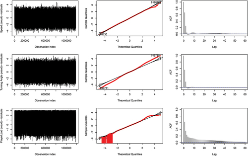
The goodness-of-fit of HMMs is typically assessed by visualizing their pseudo-residuals (Zucchini & MacDonald, 2009). These values serve the same function of assessing model fit as the residuals of traditional statistical models. Figures A7–A10 in the Appendix display plots, QQ plots and ACFs of the pseudo residuals for each data stream for the three- and five-state models.

Post-modeling analysis

The Viterbi algorithm produces a sequence of the most likely state a player was in at each time step, the “Viterbi path.” In contrast to established approaches of categorizing movement with user-defined numeric thresholds for the description of activity profiles and calculation of a player’s load, here the activity profile of players was categorized by the underlying states and the total load informed by the cumulative time spent in each state. We thus focused on visualizing activity profiles and load to support decision-making. The Viterbi path was visualized in three ways: the overall proportion of time players spent in each state, the cumulative time spent in each state across training drills and matches, and individual players’ state-decoded GPS files.

Since separate models were fit to the training and match data, the proportions of time spent in each state between the match data and training drills are not comparable. To facilitate a direct comparison of these proportions, the training model was used to predict a Viterbi path for each GPS file in the match data. As there was no heart rate covariate available for matches, we experimented with several fixed values for heart rate and discovered that it made little difference to the overall proportions in each state. Consequently, the overall mean heart rate value from the training data was used.

The derived activity states across all players were compared based on their means and standard errors within and between training and match modalities. Individual players were compared based on their cumulative time spent in each activity state and actual GPS files within and across training drills and matches.

Results

The results for only the best five-state HMM are included here. Results for the best three-state HMM are included in the Appendix.

Model fit

Apart from a lack of fit in the tails of the distributions, the models achieved satisfactory goodness-of-fit (Figures A8 & A10 in the Appendix). While the correlation between PlayerLoad and speed was high ($\sim$0.7), it was not a concern since the primary focus of fitting HMMs was on the state-switching dynamics rather than the correlation between variables or the predictive performance of the models (DeRuiter et al., 2017).

HMM categorization of player activity

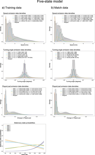
The best-fitting five-state HMMs categorized player movement into the following five states (Figure 1):

• State 1: Slow, undirected movement with low PlayerLoad. This is characteristic of movements like standing and walking around.

• State 2: Slow to moderate paced, somewhat directed movement with low PlayerLoad. This is characteristic of movements like jogging and slow running.

• State 3: For training, a mixture between moderate paced to fast, somewhat directed running with medium to high PlayerLoad. For matches, moderate paced very directed running with low PlayerLoad.

• State 4: Slow to moderate paced, undirected movement with low to medium levels of PlayerLoad. The higher levels of PlayerLoad here relative to state 1 could represent movement in contact situations.

• State 5: For training, very directed and very fast to sprinting speed in a straight line with very high PlayerLoad. For matches, very directed medium to very fast running in a straight line with high PlayerLoad.

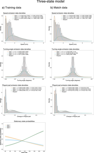
Figure 1. State distributions, with their parameter estimates and corresponding 95% confidence intervals, and stationary state probability plots for the five-state HMM fitted to the training data and the match data. For turning angle distributions, $\mathit{\sigma }$ refers to an angle concentration parameter inversely related to variance. There was no heart rate data available for the match data, hence the absence of the stationary state probability plot in Panel (b).

Influence of time-varying covariates on activity state

The stationary state probability plot (Figure 1a) displays the probability of a player transitioning to a particular state as a function of their heart rate for the training data. Initial increases in the heart rate (from 60 to $\sim$ 160) were associated with players becoming more likely to transition to the moderately fast movement state (state 3) or the slower, medium PlayerLoad state (state 4). Further increases in heart rate were associated with a transition to the fastest movement state (state 5).

Figure 2 shows the probabilities of a player transitioning to a particular state as a function of both the proportion of time elapsed and the score difference in a match for six combinations of these covariates: a) far behind on the scoreboard; b) level on the scoreboard and c) far ahead on the scoreboard; d) just over midway through the first half, e) early in the second half and f) late in the second half). These values were chosen by way of example—any values of these covariates could be chosen.

Figure 2. Stationary state probability plots for the five-state HMM, with proportion of match elapsed and score difference as transition probability covariates, fitted to the match data.

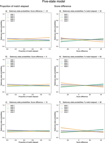
As a match progresses, the probability of transitioning to the low speed state (state 1) increases (Figure 2a), being more likely the further behind on the scoreboard the team finds itself (Figure 2a,b), while the probability of transitioning to the faster, more directed running state (state 5) decreases. The probability of transitioning to either of the moderately paced, low PlayerLoad states remains relatively constant, with the probability of transitioning to the moderate paced, medium PlayerLoad state (state 4) decreasing slightly.

As a team builds a larger lead, players are less likely to transition to the low speed state (state 1) and more likely to transition to either of the moderate paced, low PlayerLoad states (states 2 and 3). These patterns are amplified as the match progresses (Figure 2e,f). The probability of transitioning to the fastest, more directed movement state (state 5) remains relatively constant across score differences, being slightly higher overall earlier in a match.

Comparison of activity profile and load within and between training and matches

Mean speeds were generally higher in training data than in match data. The largest difference between states was that the fastest state in the training data (state 5) is associated with extremely directed, highly consistent movement (essentially sprinting in a straight line), whereas in the match data, the fastest movement state has greater variation in direction (presumably because sustained straight-line movement is rare during matches). As a result, the next fastest training state (state 3) represents a broader range of fast-moving activity (essentially, all fast movement not associated with straight-line running) than the corresponding state in the match data, which is closer to the three slower movement states (note the lower and less variable PlayerLoad associated with this state in Figure 1b).

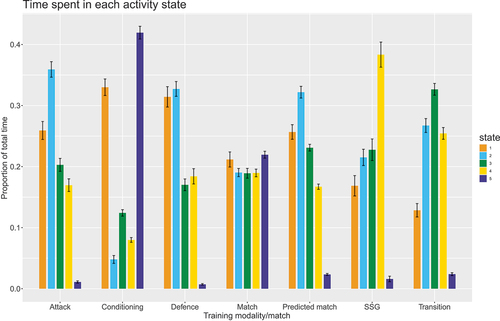
The proportion of time spent in each state varies substantially across training drills and between matches and training (Figure 3). Players spend significantly more time in the fastest state (state 5) in the conditioning drills and a very high proportion of time spent in state 4 in SSG. Players’ time is relatively evenly spread across the states in matches.

Figure 3. Proportion of time spent in each state for the five-state HMM, across all players for each training modality and the match and predicted match data.

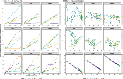
Variations in activity and load profiles, both between players (within a drill) and between drills (for the same player) are effectively visualized in plots of cumulative time spent in different states and plots of players’ movements. The activity and load profile of players can differ markedly within and across training drills (Figure 4a). For example, players spend almost no time in state 5 in the first two drills, in contrast to Broncos. Player A spends a much larger proportion of time in state 2 in arm wrestle than the other players.

Figure 4. Cumulative time spent in each state (a) and player GPS files (b) for 5-state HMM fitted to training data.

Similar variations in activity and load profiles are present within and across matches (Figure 5a). In Match (iii), Player B spends more time in state 5 and far less time in state 3 than the other players. While variation in the way players move is to be expected between matches, there is also variation in the way players move within matches. For example, in Match (iii) Player A spends relatively less time in the fastest movement state later in the game, as indicated by a slope change around two-thirds into the match.

Figure 5. Cumulative time spent in each state (a) and player GPS files (b) for 5-state HMM fitted to match data. For display purposes, only the first 500 observations (500 seconds) of the GPS files are included.

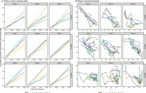
Players’ movement paths can also vary substantially between drills and matches as to how players are moving in ways representative of each state (Figure 4b). For example, the movement patterns are very similar in Broncos, but in the other drills, Player A’s movement is markedly different to the other players. There is also a significant variation in player movement paths in matches (Figure 5b). While variation within matches may be partly explained by the different playing positions, these plots still facilitate further analysis of the time and place of players’ activity profiles.

Discussion

This study aimed to demonstrate that hidden Markov models (HMMs)—a data-driven, multivariate approach—could categorize player movement into discrete states, investigate the influence of time-varying covariates on the probability of changing between these states, and investigate differences in these states between matches and training in rugby league. We have shown that HMMs, combined with appropriate visualization of their output, are a data-driven, multivariate, and statistically robust approach to profiling player activity and external load in both training and match contexts. Both three- and five-state models successfully categorized player activity into distinct states by combining multiple dimensions of player movement.

HMMs can examine the effect of time-varying covariates on in-match player activity, representing an augmentation of current activity and load profiling approaches, enabling the investigation of new important issues. While the general patterns in the effect of the heart rate covariate on player movement in training are what we expected to see, i.e., strong association (not causation) between heart rate and the probabilities for different activity states, the values at which the probabilities crossover yielded new insight. The fact that the probability of transitioning to state 3 or state 4 was almost identical for all values of heart rate suggests state 4 includes movement in contact where players are experiencing a high PlayerLoad, with associated high HRs but not moving quickly.

Similarly, for match data, some of the patterns observed (e.g., higher probability of engaging in the slower state as the match progresses—likely due to players becoming more fatigued) are to be expected. However, the reasons for other results are not immediately apparent. For example, the decreasing probability of transitioning to the slowest speed state as the scoreboard lead increases, accompanied by an increase in transitioning to the two moderately paced, low PlayerLoad states. One potential explanation for this is that winning teams retain more possession of the ball (Parmar et al., 2017) and thus spend more time running and avoiding contact with the opposition. Defending players (i.e. not in possession of the ball) have been shown to engage in more low-speed activity (T. J. Gabbett et al., 2014), which would support this explanation. More research into the effects of these and other covariates (e.g., number of tries scored or number of interchanges made by the team) on player activity is warranted.

Few studies have compared the activity profiles and load of players between training and matches. The HMM visualizations presented here can facilitate such comparisons at an individual player level in an objective way. To contrast the activity states between matches and training, we fit two separate models to those datasets. The activity states derived by the 5-state HMM show distinct differences for the two fastest-moving states. These differences are indicative of the states being data-driven, where the fastest state in training (state 5) represents very directed sprinting which occurs less frequently in matches. These demonstrable differences support the argument for individualized (Soligard et al., 2016) and/or position-specific activity profiles and load monitoring (Hausler et al., 2016). This can be addressed implicitly by contrasting individual players’ data visualizations and explicitly by including playing position as a covariate and analyzing the subsequent Viterbi paths. Including plots of the players’ GPS files provides insight into when, for how long, how frequently and where on the field players are in different states. This information could be beneficial in designing or validating training drills that aim to mimic match-day situations.

There are several ways the methodology presented here could be used to improve load monitoring. Here, we discuss two. Should reliable heart rate data be available to all players, this could be modeled as an objective measure of internal load to assist in minimizing injury risk. For example, a player may have an abnormally high heart rate which translates to them spending a much larger proportion of time in a higher activity state even though their movements appear to be the same as other players. This discrepancy may suggest behavioral change resulting from fatigue or injury. Combining this insight from the heart rate data with the player’s session rating of perceived exertion could result in the player being flagged as a potential injury risk.

Alternatively, by changing the time unit from a single training drill to an entire training session or week of training, the cumulative time spent in each state could be used to assess whether there have been any sharp increases in, or high chronic, load which is associated with increased injury risk (Soligard et al., 2016).

A major advantage of HMMs is the flexibility they enable in the choice of data streams to model, distributions to model the data streams, number of states, variables to include as covariates, and ways to visualize the Viterbi path data. For example, we experimented with multiple combinations of variables before choosing the final variables considered in this study. These variables were chosen from those available in the data and are not prescriptive. Coaches and other stakeholders may wish to model different variables and their combinations.

The HMMs fitted here had either three or five states. However, any number of states could be chosen depending on what is appropriate for the sport or the research objective; statistical criteria are available for guiding this decision, e.g., AIC. This flexibility in choice of the number of states, informed by the modeler’s domain knowledge and the research objective stands in contrast to the approach of pre-defined thresholds for categorizing activity states as the resulting state distributions are data-driven and derived from multiple variables (Dalton-Barron et al., 2020). Thus, the approach detailed in this study has the potential to address some of the recent concerns raised around univariate, threshold-based approaches where the lack of agreement on, and absence of, standardized thresholds makes it difficult to compare activity profiles or load across sports and studies (Sweeting et al., 2017).

Since the approach adopted here is multivariate, data-driven and focused on data visualization, it can become a standardized method for analyzing player activity and load across many different sports (Bourdon et al., 2017) that considers the specific demands of each sport (Lambert & Borresen, 2010), each of which may have unique variables of interest in addition to those that are common. For example, if the research question was to compare the activity profiles and load between players across different (a) modalities within a sport or (b) different sports with some common movement variables, one model could be fit to all the data. The players’ Viterbi path visualizations could then be contrasted, focusing on the time spent in each state between players from different sports.

We demonstrated one way the comparisons for (a) could be made in Figure 3 with the Predicted Match time-in-state proportions by showing the proportion of overall time spent in each movement state. Although none of the proportions of time spent across states in any drill closely resembles the predicted match data proportions, it is possible to find a selection of drills whose combined distribution best matches that of the predicted match data, to adequately prepare players for match demands.

To our knowledge, this is the first study to use data visualization to facilitate such decision support (Bourdon et al., 2017). The envisaged application of the methodology employed in this paper would be a decision support system that coaches and other stakeholders could use to produce only the player-specific visualizations to facilitate insight and discussion, i.e. it would not be necessary or advisable to display the figures relating to HMMs themselves. These visualizations represent an objective method of assessing whether players are being adequately prepared to meet match demands (T. Gabbett et al., 2008; Hogarth et al., 2016) and can readily be tailored to detect meaningful changes in activity profiles or load at the individual, position, or team level (Bourdon et al., 2017; Halson, 2014) while remaining scientifically valid due to the robust underlying statistical model. They can thus provide decision support by informing coaches as to which drills, and their periodization will be most effective in preparing players for optimal performance.

Limitations

This study was limited to data being available for only one team and no heart rate data being present for match player GPS files which prevented richer comparisons between training and match activity states. Caution should thus be exercised when generalizing these results in rugby league. The effect of the playing position on the derived activity states was also not explored. The approach used in this study can thus be augmented by including playing position as a covariate or fitting separate HMMs for each playing position. Further work could also be done by considering measures of internal load, e.g., session rating of perceived exertion and combining objective and subjective measures of load (Bourdon et al., 2017; Soligard et al., 2016; Weaving et al., 2017). For example, players’ sRPEs for a training drill could be compared with the cumulative time spent in each state.

Conclusion

HMMs are a data-driven, flexible, multivariate method for effectively profiling player activity and load in rugby league. They can model the inherent complexity of player movement and the influence of time-varying covariates on player activity, as well as facilitate objective comparison of activity and load profiles between training and match contexts. While in this paper we have focused on the use of HMMs in rugby league, throughout we have emphasized the flexibility of the approach. All that is required to use the approach detailed here is movement data derived from, e.g., GPS trackers, potentially augmented by other wearable devices. A wide variety of research hypotheses can be tackled using the same basic statistical framework, making HMMs a potentially useful tool for several other sports.

Disclosure statement

No potential conflict of interest was reported by the author(s).

Additional information

Funding

The work was supported by the National Research Foundation of South Africa and the Department of Higher Education and Training via the Teaching and Development Grant (IRMA: 29113).

Appendix

Model selection and fit

Table A1. AIC values for fitted models.

Model	Data	Num. States	Covariate	AIC	Akaike Weight
m_train3	Training	3		422327	0
m_train3_hr	Training	3	Heart rate	420551	0
m_train5	Training	5		20218	0
m_train5_hr	Training	5	Heart rate	18175	1
m_match3_time	Match	3	Time in game	−237315	0
m_match3	Match	3		−329777	0
m_match3_score	Match	3	Score difference	−330290	0
m_match3_score_time	Match	3	Score difference and Time in game	−330560	1
m_match5	Match	5		−1241251	0
m_match5_time	Match	5	Time in game	−1241547	0
m_match5_score	Match	5	Score difference	−1242116	0
m_match5_score_time	Match	5	Score difference and Time in game	−1242405	1

GPS quality

Figure A1. Examples of (a) GPS les with good quality that were retained and (b) GPS les with poor quality that were removed after visual inspection.

Three-state HMM results

HMM categorization of player activity

 The best-fitting three-state HMM categorized player movement into the following three states (Figure A2, training data Panel A, match data Panel B):

• State 1: Slow, undirected movement with low PlayerLoad. This is characteristic of movements like standing and walking around.

• State 2: Moderate paced, directed movement with low PlayerLoad. This is characteristic of movements like jogging and slow running in a straight line.

• State 3: Moderate to fast paced, somewhat directed movement with medium to high PlayerLoad. This is characteristic of movements like fast, directed running, sprinting and evasive (i.e., side-to-side) maneuvers. This could also represent movement in contact situations where PlayerLoad is high, but the speed of movement is low.

Figure A2. State distributions, with their parameter estimates and 95% confidence intervals for those estimates, and stationary state probability plots for the three-state HMM fitted to the training data (Panel a) and the match data (Panel b). For turning angle distributions, σ refers to an angle concentration parameter inversely related to variance. There was no heart rate data available for the match data, hence the absence of the stationary state probability plot in Panel b.

The influence of time-varying covariates on activity state

The stationary state probability plot (Figure A2a) displays the probability of a player transitioning a particular state as a function of their heart rate for the training data. An increase in heart rate corresponds to a similar decrease in the probability of transitioning to either of the two slower states and a steep increase in the likelihood of transitioning to the fastest state (state 3). There is a roughly equal chance of transitioning to any one of the three states when the heart rate is approximately 130 beats per minute.

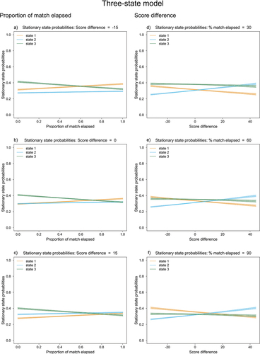
Figure A3 shows the probabilities of a player transitioning to a particular state as a function of both the proportion of time elapsed and the score difference in a match for six combinations of these covariates a) far behind on the scoreboard; b) level on the scoreboard and c) far ahead on the scoreboard; d) just over midway through the first half, e) early in the second half and f) late in the second half).

As a match progresses, players are less likely to transition to the fast speed state (state 3) and more likely to transition to the low speed state (state 1). The probability of engaging in the moderate paced, directed movement state (state 2) increases marginally as the match progresses and is higher the larger the scoreboard lead.

The further ahead a team is on the scoreboard, the less likely they are to engage in the low speed and low PlayerLoad state (state 1), although the probability of transitioning to this state is slightly higher across score differences later in the match (Figure A3d-f). Conversely, players are increasingly likely to transition to the moderate paced, directed running state (state 2) as the team builds a larger point lead, independent of the time elapsed in the match.

Comparison of activity profile and load within and between training and matches

Similar movement states were observed in models fitted to training data (Figure A2a) and match data (Figure A2b), especially the speed of movement. Player movement was generally more directed at matches than in training.

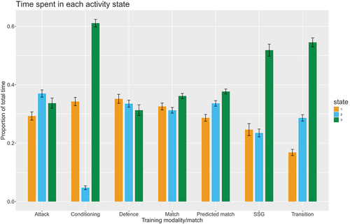
The proportion of time spent in each state differs substantially between the matches and the training drills and across the different training modalities (Figure A4). The most striking difference is the high proportion of time spent in state 3 for conditioning, small-sided games and transition modalities. One would expect this result for the conditioning drills as these often involve sprinting at maximum capacity, but it is less clear why drills from other modalities also show large proportions of time spent in the fastest state.

Figure A3. Stationary state probability plots for the three-state HMM, with proportion of match elapsed and score difference as transition probability covariates, fitted to the match data.

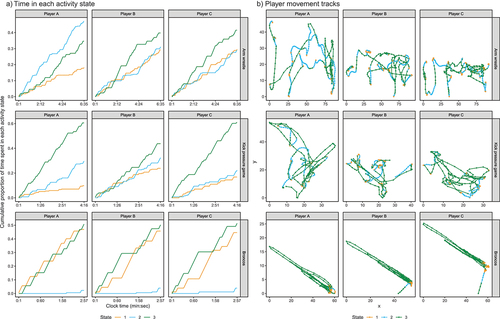
The load and activity profile of players can differ markedly within a drill (Arm wrestle and Kick pressure game) and across training drills (Figure A5a). For example, players spend very little time in state 2 in Broncos compared to the other drills, while in Kick pressure games, Player B’s time is much more evenly spread across the three states than the other two players.

Figure A4. Proportion of time spent in each state for the three-state HMM, across all players for each training modality and for the match and predicted match data. The predicted match file was obtained by using the training model with the overall mean value for the heart rate covariate to predict the Viterbi sequence for each match data player’s GPS file.

The broad movements players undertake can vary substantially between drills as to when and in what area of the field players are moving in ways representative of each state (Figure A5b). For example, in Broncos the players are all engaging in movement, representing each state at a similar time and place. However, in the other drills, there is more variation between the players’ representative movements.

Similar variations in activity profiles and load are present in the match data (Figure A6a). While the cumulative time spent in each state (Panel A) within a match is similar across players in the first two matches, in Match (iii) there are striking differences between Players A and B. Player B spends a larger proportion of time in state 3 than both other players, while Player A spends a larger proportion of time in state 2.

Figure A5. Cumulative time spent in each state (a) and player GPS files (b) for 3-state HMM fitted to training data.

These three players move differently within and across matches, reflected in the time and place their movement represents the different states (Figure A6b). These differences in activity profiles and load between players and across matches can be partly explained by different playing positions and the natural variation in player movement from match to match.

Figure A6. Cumulative time spent in each state (a) and player GPS files (b) for 3-state HMM fitted to match data. For display purposes, only the first 500 observations (500 seconds) of the GPS les are included.

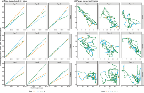
Figure A7. Pseudo-residual plots for three-state HMM fit to the training data.

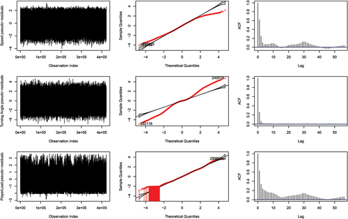
Figure A8. Pseudo-residual plots for five-state HMM fit to the training data.

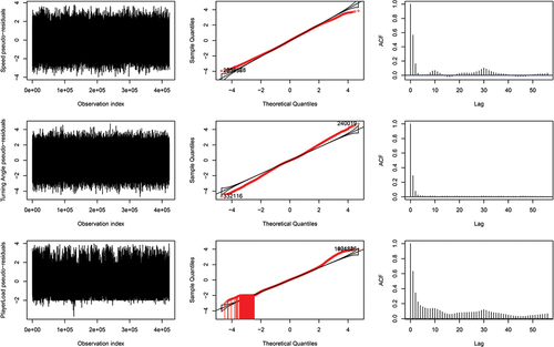
Figure A9. Pseudo-residual plots for three-state HMM fit to the match data.

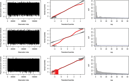
Figure A10. Pseudo-residual plots for five-state HMM fit to the match data.

References

- Akaike, H. (1987). Factor analysis and AIC. Psychometrika, 52, 317–332.
- Barkell, J. F., Pope, A., OConnor, D., & Cotton, W. G. (2017). Predictive game patterns in world rugby sevens series games using Markov chain analysis. International Journal of Performance Analysis in Sport, 17(4), 630–641. https://doi.org/10.1080/24748668.2017.1381459
- Bourdon, P. C., Cardinale, M., Murray, A., Gastin, P., Kellmann, M., Varley, M. C., Gabbett, T. J., Coutts, A. J., Burgess, D. J., Gregson, W., & Cable, N. T. (2017). Monitoring athlete training loads: Consensus statement. International Journal of Sports Physiology and Performance, 12(s2), S2–S161. https://doi.org/10.1123/IJSPP.2017-0208
- Boyd, L. J., Ball, K., & Aughey, R. J. (2011). The reliability of minimaxX accelerometers for measuring physical activity in Australian football. International Journal of Sports Physiology and Performance, 6(3), 311–321. https://doi.org/10.1123/ijspp.6.3.311
- Collins, N., White, R., Palczewska, A., Weaving, D., Dalton-Barron, N., & Jones, B. (2022). Moving beyond velocity derivatives; using global positioning system data to extract sequential movement patterns at different levels of rugby league match-play. European Journal of Sport Science, 1–23. https://doi.org/10.1080/17461391.2022.2027527
- Dalton-Barron, N., Whitehead, S., Roe, G., Cummins, C., Beggs, C., & Jones, B. (2020). Time to embrace the complexity when analysing gps data? A systematic review of contextual factors on match running in rugby league. Journal of Sports Sciences, 38(10), 1161–1180. https://doi.org/10.1080/02640414.2020.1745446
- DeRuiter, S. L., Langrock, R., Skirbutas, T., Goldbogen, J. A., Calambokidis, J., Friedlaender, A. S., & Southall, B. L. (2017). A multivariate mixed hidden Markov model for blue whale behaviour and responses to sound exposure. The Annals of Applied Statistics, 11(1), 362–392. https://doi.org/10.1214/16-AOAS1008
- Fox, J. L., Stanton, R., Sargent, C., Wintour, S.-A., & Scanlan, A. T. (2018). The association between training load and performance in team sports: A systematic review. Sports Medicine, 48(12), 2743–2774. https://doi.org/10.1007/s40279-018-0982-5
- Gabbett, T. J. (2015). Relationship between accelerometer load, collisions, and repeated high-intensity effort activity in rugby league players. The Journal of Strength & Conditioning Research, 29(12), 3424–3431. https://doi.org/10.1519/JSC.0000000000001017
- Gabbett, T. J., Polley, C., Dwyer, D. B., Kearney, S., & Corvo, A. (2014). Influence of field position and phase of play on the physical demands of match-play in professional rugby league forwards. Journal of Science and Medicine in Sport, 17(5), 556–561. https://doi.org/10.1016/j.jsams.2013.08.002
- Gabbett, T., King, T., & Jenkins, D. (2008). Applied physiology of rugby league. Sports Medicine, 38(2), 119–138. https://doi.org/10.2165/00007256-200838020-00003
- Halson, S. L. (2014). Monitoring training load to understand fatigue in athletes. Sports Medicine, 44(2), 139–147. https://doi.org/10.1007/s40279-014-0253-z
- Hausler, J., Halaki, M., & Orr, R. (2016). Application of global positioning system and microsensor technology in competitive rugby league match-play: A systematic review and meta-analysis. Sports Medicine, 46(4), 559–588. https://doi.org/10.1007/s40279-015-0440-6
- Higham, D. G., Pyne, D. B., Anson, J. M., Hopkins, W. G., & Eddy, A. (2016). Comparison of activity profiles and physiological demands between international rugby sevens matches and training. The Journal of Strength & Conditioning Research, 30(5), 1287–1294. https://doi.org/10.1519/JSC.0b013e3182a9536f
- Hogarth, L. W., Burkett, B. J., & McKean, M. R. (2016). Match demands of professional rugby football codes: A review from 2008 to 2015. International Journal of Sports Science & Coaching, 11(3), 451–463. https://doi.org/10.1177/1747954116645209
- Howe, S. T., Aughey, R. J., Hopkins, W. G., & Stewart, A. M. (2023). Profiling professional rugby union activity after peak match periods. International Journal of Sports Physiology and Performance, 18(9), 968–981. https://doi.org/10.1123/ijspp.2023-0028
- Hulin, B. T., Gabbett, T. J., Johnston, R. D., & Jenkins, D. G. (2018). Playerload variables: Sensitive to changes in direction and not related to collision workloads in rugby league match play. International Journal of Sports Physiology and Performance, 13(9), 1136–1142. https://doi.org/10.1123/ijspp.2017-0557
- Kelly, V. G., & Coutts, A. J. (2007). Planning and monitoring training loads during the competition phase in team sports. Strength & Conditioning Journal, 29(4), 32–37. https://doi.org/10.1519/00126548-200708000-00005
- Kempton, T., Sirotic, A. C., & Coutts, A. J. (2017). A comparison of physical and technical performance profiles between successful and less-successful professional rugby league teams. International Journal of Sports Physiology and Performance, 12(4), 520–526. https://doi.org/10.1123/ijspp.2016-0003
- Lambert, M. I., & Borresen, J. (2010). Measuring training load in sports. International Journal of Sports Physiology and Performance, 5(3), 406–411. https://doi.org/10.1123/ijspp.5.3.406
- Langrock, R., King, R., Matthiopoulos, J., Thomas, L., Fortin, D., & Morales, J. M. (2012). Flexible and practical modeling of animal telemetry data: Hidden Markov models and extensions. Ecology, 93(11), 2336–2342. https://doi.org/10.1890/11-2241.1
- Loader, J., Montgomery, P. G., Williams, M. D., Lorenzen, C., & Kemp, J. G. (2012). Classifying training drills based on movement demands in Australian football. International Journal of Sports Science & Coaching, 7(1), 57–67. https://doi.org/10.1260/1747-9541.7.1.57
- Marino, T. K., Ferreira, A. R., Morgans, R., Schildberg, W. T., Aoki, M. S., Corrȇa, U. C., & Moreira, A. (2022). The emergence of critical incidents in rugby union matches using Markov chain analysis. Science and Medicine in Football, 1–8. https://doi.org/10.1080/24733938.2022.2135758
- McClintock, B. T., & Michelot, T. (2018). momentuHMM: R package for generalized hidden Markov models of animal movement. Methods in Ecology and Evolution, 9(6), 1518–1530. https://doi.org/10.1111/2041-210X.12995
- McGarry, T., & Franks, I. M. (1996). Development, application, and limitation of a stochastic Markov model in explaining championship squash performance. Research Quarterly for Exercise and Sport, 67(4), 406–415. https://doi.org/10.1080/02701367.1996.10607972
- Motoi, S., Misu, T., Nakada, Y., Yazaki, T., Kobayashi, G., Matsumoto, T., & Yagi, N. (2012). Bayesian event detection for sport games with hidden Markov model. Pattern Analysis and Applications, 15(1), 59–72. https://doi.org/10.1007/s10044-011-0238-6
- Newton, P. K., & Aslam, K. (2009). Monte carlo tennis: A stochastic Markov chain model. Journal of Quantitative Analysis in Sports, 5(3). https://doi.org/10.2202/1559-0410.1169
- Ötting, M., Langrock, R., & Maruotti, A. (2021). A copula-based multivariate hidden Markov model for modelling momentum in football. AStA Advances in Statistical Analysis, 1–19. https://doi.org/10.1007/s10182-021-00395-8
- Parmar, N., James, N., Hughes, M., Jones, H., & Hearne, G. (2017). Team performance indicators that predict match outcome and points difference in professional rugby league. International Journal of Performance Analysis in Sport, 17(6), 1044–1056. https://doi.org/10.1080/24748668.2017.1419409
- R Core Team. (2021). R: A language and environment for statistical computing. R Foundation for Statistical Computing. https://www.R-project.org/
- Soligard, T., Schwellnus, M., Alonso, J.-M., Bahr, R., Clarsen, B., Dijkstra, H. P., Gabbett, T., Gleeson, M., Hägglund, M., Hutchinson, M. R., Janse van Rensburg, C., Khan, K. M., Meeusen, R., Orchard, J. W., Pluim, B. M., Raftery, M., Budgett, R., & Engebretsen, L. (2016). How much is too much? (part 1) International Olympic Committee consensus statement on load in sport and risk of injury. British Journal of Sports Medicine, 50(17), 1030–1041. https://doi.org/10.1136/bjsports-2016-096581
- Sweeting, A. J., Cormack, S. J., Morgan, S., & Aughey, R. J. (2017). When is a sprint a sprint? A review of the analysis of team-sport athlete activity profile. Frontiers in Physiology, 8(432). https://doi.org/10.3389/fphys.2017.00432
- Tee, J. C., Lambert, M. I., & Coopoo, Y. (2016). GPS comparison of training activities and game demands of professional rugby union. International Journal of Sports Science & Coaching, 11(2), 200–211. https://doi.org/10.1177/1747954116637153
- Viterbi, A. (1967). Error bounds for convolutional codes and an asymptotically optimum decoding algorithm. IEEE Transactions on Information Theory, 13(2), 260–269. https://doi.org/10.1109/TIT.1967.1054010
- Walsh, J., Heazlewood, I., & Climstein, M. (2012). Modelling touch football (touch rugby) as a Markov process. International Journal of Sports Science and Engineering, 6, 203–212.
- Weaving, D., Jones, B., Marshall, P., Till, K., & Abt, G. (2017). Multiple measures are needed to quantify training loads in professional rugby league. International Journal of Sports Medicine, 38(10), 735–740. https://doi.org/10.1055/s-0043-114007
- White, R., Palczewska, A., Weaving, D., Collins, N., & Jones, B. (2022). Sequential movement pattern-mining (SMP) in field-based team-sport: A framework for quantifying spatiotemporal data and improve training specificity? Journal of Sports Sciences, 40(2), 164–174. https://doi.org/10.1080/02640414.2021.1982484
- Xiong, Z. (2005). Audio-visual sports highlights extraction using coupled hidden Markov models. Pattern Analysis and Applications, 8(1–2), 62–71. https://doi.org/10.1007/s10044-005-0244-7
- Zucchini, W., & MacDonald, I. L. (2009). Hidden Markov models for time series: An introduction using R. Chapman and Hall/CRC.