Growth responses and adaptations of the emergent macrophyte Acorus calamus Linn. to different water-level fluctuations

Abstract

Acorus calamus Linn. was grown under four water-level fluctuation (WLF) treatments to study the influence of WLF on the growth of the species. The four WLF treatments (designated as 0 cm, 60 cm, 60 ± 30 cm, and 60 ± 60 cm) were initiated with the minimum water levels (0, 60, 30, and 0 cm, respectively) for a week and then switched to the maximal water levels (0, 60, 90, and 120 cm, respectively) one week later. This cycle was repeated six times during 12 weeks. Relative growth rate (RGR), biomass allocation, shoot and below-ground morphology, chlorophyll content, and concentrations of proline, malondialdehyde (MDA), and soluble sugar (SS) of A. calamus were measured. After the 12 weeks' WLF treatment, growth rate differed among the treatments. RGR was negative in the 60 cm treatment. A. calamus showed significant morphological adaptations to WLFs, including different patterns in length, blade length, width and numbers of shoots. The root:shoot ratio was significantly greater in the 0 cm treatment with no significant differences among the other three WLF treatments. SS concentrations in the rhizome and root were higher in the 60 ± 60 cm treatment than in either the 60 cm treatment or 60 ± 30 cm treatment. No clear relationship was found among the treatments for chlorophyll concentrations, proline, or MDA concentrations in the shoots but fluctuating water levels significantly stimulated proline and MDA accumulation. The differences in biomass and morphological variables among treatments suggested that WLF is an important regulator of the growth of A. calamus and that the species is better adapted to cyclic WLFs than to constant deep water.

Keywords:

• water-level fluctuations
• biomass production
• biomass allocation
• shoot morphology
• root morphology
• Acorus calamus

Introduction

In wetlands, ponds, and regulated systems, several components of the hydrologic regime (not simply instantaneously measured water depth) have been implicated in affecting the composition, diversity, and distribution of macrophyte communities (Casanova & Brock 2000; Kennedy et al. 2003; Nicol et al. 2003; Boar 2006) as well as physiological changes within individual plants. For example, the response of emergent species to an increase in water level, often, is the allocation of biomass to above-ground tissues in order to maintain access to atmospheric carbon dioxide (Squires & van der Valk 1992; Cooling et al. 2001; Deegan et al. 2007). Such water-level fluctuations (WLFs) are commonly associated with the tail waters in main river channels below locks and weirs in regulated river systems (Blanch et al. 2000). However, WLFs can occur quickly and plants may not have time to morphologically adjust to rising water levels before water levels change once again, requiring a different set of responses to optimize growth (Vretare et al. 2001). Rapid cyclic fluctuations in water level, therefore, may result in intermittent periods of resource limitation, where the degree of limitation should be commensurate with the amplitude of WLFs.

Emergent macrophytes growing in the littoral zone are often subjected to WLFs caused by flooding or human regulation (Wantzen et al. 2008), making it important to understand their growth responses and adaptation mechanisms to WLFs. Acorus calamus Linn. is an amphibious plant that is common in China and adapted to periods of flooding and the consequent hypoxic conditions as a part of its natural life cycle. The use of this species in constructed wetlands for wastewater treatment (Caicedo et al. 2000; Clarke & Baldwin 2002) in China is another reason to study its growth. Some previous studies have investigated growth responses and morphological adaptations of A. calamus to average water depth. Ordinarily, emergent macrophytes adjust to a 60 cm water depth and the ensuing limitations in carbon dioxide and oxygen through morphological plasticity, specifically, an elongation of the shoot to maintain an emergent canopy (Grace 1989; Rea & Ganf 1994; Blanch et al. 1999) and an increase in the dimensions of the lacunae to increase aeration potential (White & Ganf 1998; Sorrell & Tanner 2000). However, because average depth does not contain information about the range of depths or any extreme events, our understanding of the influence of WLFs on this species remains incomplete. The aims of this study were to determine the responses and adaptations of A.calamus to simple WLFs and whether or not the proline, malondialdehyde (MDA), chlorophyll a, and soluble sugar (SS) concentrations were affected by WLFs.

Methods

The plants used in this study were 20-cm-long seedlings of A. calamus propagated from 2- to 3-cm-long rhizome cuttings from the Guanqiao experimental laboratory of the Institute of Hydrobiology, Chinese Academy of Sciences, China. Seedlings were planted in plastic pots (18 cm diameter × 20 cm height) filled with sediment collected from Donghu Lake [total nitrogen (TN) = 3.894 ± 0.152 mg g⁻¹ DW (dry weight), total phosphorus (TP) = 1.357 ± 0.028 mg g⁻¹ DW, and organic matter = 7.032 ± 0.194%, mean ± standard deviation (SD), n = 6] to the height of 15 cm (one seedling per pot). Seedlings were weighed as fresh weight (g FW) and then the values were converted into dry weight for relative growth rate (RGR) calculations.

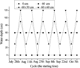
The pots planted with A. calamus seedlings were placed in outdoor ponds (3.0 m long× 1.4 m wide × 1.5 m deep) and covered with different water depths. Each treatment was replicated three times. Four WLF treatments were chosen: 0 cm, 60 cm, 60 ± 30 cm, and 60 ± 60 cm (Figure 1). All four treatments were initiated with their minimum water levels (0, 60, 30, and 0 cm, respectively) and then switched to their respective maximum levels (0, 60, 90, and 120 cm) one week later. Thus, each WLF cycle lasted for 2 weeks (Figure 1) and the experiment lasted for 12 weeks.

Figure1. A graph of the experimental system with water depth (cm) on the y-axis. Each treatment was replicated three times in outdoor ponds (3.0 m long × 1.4 m wide × 1.5 m deep) and the water levels in the fluctuating depth treatments occurred every week.

Several environmental variables were monitored during the experiment. The characteristics of the underwater light in the ponds were recorded every three days at each water level using a ZDS-10 luminometer (Shanghai, China). In situ profiles of temperature, pH, dissolved oxygen (DO), turbidity, specific conductivity, and depth were taken in each pool using a portable water-quality analyzer (5-STAR, Thermo-Orion, http://www.thermoscientific.com). Water samples were analyzed for total phosphate, TN and chlorophyll a in accordance with standard methods (Water Environment Protection Directory, China's Ministry of Environmental Protection).

Morphological variables of the plants, including shoot number, shoot width, shoot length, and shoot blade length, were measured in every cycle. Meanwhile, the proline, MDA, chlorophyll a, and SS concentrations in leaves were also measured as described below. At the end of the experiment, the plants were harvested and the damaged shoots were separated. All plants were divided into shoots (live and yellow), rhizomes, and roots and then washed free of sediment with tap water. Dry weights of individual tissues were determined after drying to a constant weight at 80°C for determination of biomass production. A detailed morphometric analysis of underground structures was conducted, including total length of the rhizome, and number, length, and diameter of the individual roots.

The proline concentrations were determined following the procedure of Bates et al. (1973): 0.500 g of the plant tips were homogenized in 3% aqueous sulfosalicylic acid and the homogenates were centrifuged at 10,000 rpm. The reaction mixture consisting of 2 mL supernatant, 2 mL acid ninhydrin (1.2 g ninhydrin in 30 mL glacial acetic acid and 20 mL of 6 M orthophosphoric acid), and 2 mL of glacial acetic acid was boiled at 100°C for 1 h. The reaction was terminated over an ice bath. The reaction mixture was extracted with 4 mL toluene, and absorbance of the toluene fraction was read at 520 nm in a spectrophotometer (Daojin UV-1800).

MDA concentrations were measured as follows: 0.500 g plant material was homogenized with 3 mL of 0.5% thiobarbituric acid in 20% tri-chloroacetic acid (w/v). The homogenate was incubated at 100°C for 30 min and the reaction was stopped in ice water. The samples were centrifuged at 10,000 rpm for 10 min and absorbance was recorded at 450, 532, and 600 nm. The MDA concentration was determined by the following formula: C_MDA (μmol L⁻¹) = 6.45 (A₅₃₂ − A₆₀₀) − 0.56 A₄₅₀, from which the absolute concentration (mg g⁻¹ FW) of MDA was calculated (Li 2000).

For the chlorophyll a analysis, 0.100 g finely chopped fresh leaves were placed in a capped tube containing 25 mL of 80% acetone and placed inside a refrigerator (4°C) for 28 h (Sarkar 1998). The chlorophyll a was measured spectrophotometrically following Porra (2002).

For SS, 0.100 g dried powder of shoot samples was extracted in distilled water by boiling at 100°C on a water bath for 30 min twice, adjusted to constant volume of 25 mL and mixed. Subsequent to cooling, the supernatant was decanted following centrifugation and then, after appropriate dilutions, heated with 0.5 mL anthrone reagent and 5 mL concentrated sulfuric acid and immediately cooled. Absorbance was measured by a spectrophotometer at 630 nm.

Biomass production was measured as RGR and was calculated according to the following equation at each water depth:

where W₁ and W₂ were the initial and final plant dry weights, respectively, and t₁ and t₂ were the initial and final experimental time (days) , respectively.

R:S is the ratio of root dry matter to shoot dry matter production. The yellow shoot ratio is the ratio of damaged shoot biomass to the total biomass. Data presented were the means ± SD of the triplicates. One-way ANOVA followed by Duncan's test was performed to confirm the validity of results and the significant difference among treatments. Significance was set at 0.05 (SPSS 13.0 for Windows).

Results

The average water physicochemical parameters are presented in Table 1. The average water temperature in the ponds was 28.6 ± 1.73°C (range = 26.5–30.3°C). The average light intensities of the ponds were 4146 ± 674 lx. The TN and TP concentrations were 2.20 ± 0.580 and 0.395 ± 0.097 mg L⁻¹, respectively. The water conditions were suitable for the growth of A. calamus.

Table1 Water physical and chemical conditions during the experiment.

Parameter	Mean ± SD	Range
Water temperature (°C)	28.6 ± 1.7	26.5–30.3
Illumination (lx)	4146 ± 674	2831–6067
pH	7.69 ± 0.51	6.53–7.91
Total suspended solid (TSS) (mg L^−1)	2.28 ± 0.47	2.08–2.37
DO (mg L^−1)	8.22 ± 0.32	7.90–8.36
Chl a (μg L^−1)	1.53 ± 0.47	1.41–1.98
Electrical conductivity (EC) (μS cm^−1)	247.3 ± 8.3	222.5–278.4
Total dissolved solid (TDS) (mg L^−1)	760.2 ± 1.3	758.3–763.9
Transparency SD (cm)	107.8 ± 23.1	92.3–150.0
Oxidation-reduction potential (ORP) (mV)	−98.7 ± 11.2	−82.2 to –130.9
Turbidity [Nephelometric turbidity unit (NTU)]	1.95 ± 0.63	1.39–2.35
TN (mg L^−1)	2.20 ± 0.58	1.92–2.54
TP (mg L^−1)	0.395 ± 0.097	0.220–0.405

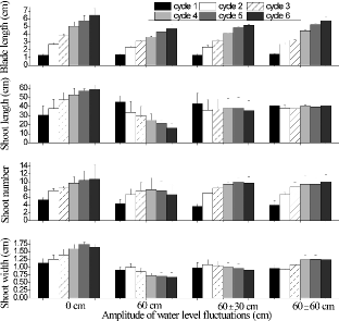
Although no clear relationship was found between WLFs and shoot morphology, there was a trend suggesting that WLFs could be important in determining shoot morphology. At the end of the experiment, the shoot length of A. calamus was the greatest in the 0 cm treatment (Figure 2). The shoot number, shoot width, and shoot blade length also showed the largest increases in the 0 cm treatment. In the 60 ± 60 cm treatment, the shoot width increased from an initial 0.963 ± 0.110 cm to 1.237 ± 0.100 cm at the end, and the shoot length increased from 40.83 ± 0.577 cm to 41.1 ± 2.51 cm. The trend in shoot length was obviously opposite in the 60 ± 0 cm treatment where it decreased in a near linear fashion from 45.0 ± 6.93 cm to 16.5 ± 5.0 cm. The shoot number at 60 ± 0 cm first increased up to the fourth cycle and then decreased thereafter to the lowest value of all treatments (Figure 2).

Figure2. Changes in mean blade length, shoot length, shoot number, and shoot width per pot over time in Acorus calamus subjected to four water-level fluctuation treatments (0 cm, 60 cm, 60 ± 30 cm, and 60 ± 60 cm). Each cycle was 2 weeks in duration.

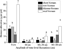
After the 12 weeks' WLF treatments, shoot biomass, rhizome biomass, root biomass, and total biomass differed among the treatments (F_3,8 = 32.15, p < 0.001; F_3,8 = 74.01, p < 0.001; F_3,8 = 21.66, p < 0.001; F_3,8 = 67.83, p < 0.001, respectively). Plants at 0 cm produced significantly more biomass than the other three treatments with 58.0 ± 6.4 g per pot, followed by the 60 ± 60 cm treatment with 25.76 ± 8.51 g, which were higher than the biomass produced in the 60 cm and 60 ± 30 cm treatments (Figure 3). Also, the above- and below-ground biomass of the plants were significantly different in response to the experimental WLFs (Figure 3). The shoot biomass and root biomass were both the highest in the 0 cm treatment. The rhizome biomass was significantly higher in the 0 cm and 60 ± 60 cm treatments than in the 60 ± 0 cm and 60 ± 30 cm treatments.

Figure3. Changes in total biomass and biomass allocation of Acorus calamus subjected to four water-level fluctuation treatments (0 cm, 60 cm, 60 ± 30 cm, and 60 ± 60 cm). All the values were means of triplicates ± SD. Different letters within a tissue category signify significant differences.

A. calamus had a higher proportion of biomass allocated to roots (root:shoot) in the 0 cm treatment than that in the other treatments (F_3,8 = 20.53, p < 0.001). The root:shoot ratio was 0.453 ± 0.048, 0.471 ± 0.121, and 0.382 ± 0.083 in the 60 cm, 60 ± 30 cm, and 60 ± 60 cm treatments, respectively, with no significant differences among them (Figure 4). Moreover, different WLFs had significant influences on the yellow shoot ratio (F_3,5 = 18.22, p < 0.05). The highest yellow shoot ratio was observed in the 60 cm treatment with 0.636 ± 0.173, followed by 60 ± 30 cm and 60 ± 60 cm treatments with yellow shoot ratios of 0.498 ± 0.059 and 0.318 ± 0.062, respectively, which were significantly higher than that at 0 cm (Figure 4, middle panel). None of the 60 ± 30 cm or 60 ± 60 cm treatment plants had completely died after 3 months, but approximately 40% of the plants were dead in the 60 cm treatment.

Figure4. Differences in mean ratio of root dry matter to shoot dry matter production (R:S, top panel), mean fractional number of chlorotic leaves (yellow leaf ratio, middle panel), and mean relative growth rate (RGR, bottom panel) in Acorus calamus subjected to four water-level fluctuation treatments (0 cm, 60 cm, 60 ± 30 cm, and 60 ± 60 cm). Error bars represent 1 SD. Different letters within a graph indicate significant differences among treatments.

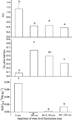
RGR, measured as change in DW per day, differed considerably among the treatments (F_3,8 = 76.53, p < 0.001; Figure 4, bottom panel). The highest value was observed at 0 cm with 24.65 ± 4.02 mg DW g⁻¹ d⁻¹, followed by the 60 ± 60 cm treatment with 15.23 ± 2.01 mg DW g⁻¹ d⁻¹, both of which were significantly higher than that of the 60 ± 30 cm treatment. The lowest value was in the 60 cm treatment which had a negative RGR.

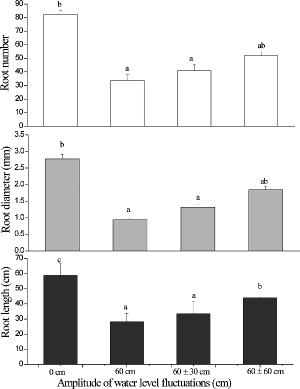
The number, length, and diameter of rhizomes in the 0 cm treatment were all significantly greater than in the other treatments (F_3,8 = 16.2, p < 0.05; F_3,8 = 12.4, p < 0.05; F_3,8 = 5.17, p < 0.05, respectively; Figure 5) with the exception of rhizome diameter in the 60 ± 60 cm treatment. There were no significant differences among the 60 cm, 60 ± 30 cm, and 60 ± 60 cm treatments. The root patterns were very similar to those of the rhizomes. The root length was the greatest in the 0 cm treatment, followed by the 60 ± 60 cm treatment, which was significantly higher than that in the 60 cm and 60 ± 30 cm treatments (F_3,8 = 97.2, p < 0.001; Figure 6). The average root diameter in the 0 cm treatment was significantly greater than those in the 60 cm and 60 ± 30 cm treatments but the diameter of roots in the 60 ± 60 cm treatment was intermediate and not significantly different from the others. The average root number in the 0 cm treatment was significantly greater than that in the 60 cm and 60 ± 30 cm treatments but not the 60 ± 60 cm treatment.

Figure5. The length, diameter and number of rhizomes in Acorus calamus subjected to four water-level fluctuation treatments (0 cm, 60 cm, 60 ± 30 cm, and 60 ± 60 cm). All the values were means of triplicates ± SD. Different letters within a graph indicate significant differences among treatments.

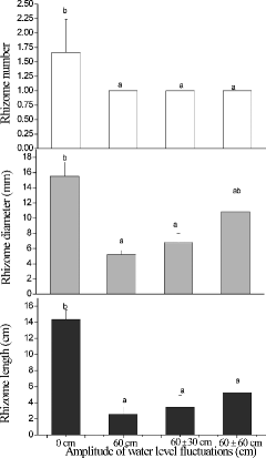
Figure6. The length, diameter and number of roots in Acorus calamus subjected to four water-level fluctuation treatments (0 cm, 60 cm, 60 ± 30 cm, and 60 ± 60 cm). All the values were mean of triplicates ± SD. Different letters within a graph indicate significant differences among treatments.

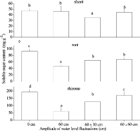
Large accumulations of proline and MDA took place in shoots of A. calamus exposed to flooded conditions. Proline concentrations generally peaked during the first cycle and declined thereafter with time (Figure 7). The highest proline concentration was found in the 60 cm treatment during the first cycle. In general, MDA concentrations were greater under flooded conditions than in the 0 cm treatment, and values during the first three cycles were mostly greater than those during the last three cycles (Figure 7). WLFs resulted in significant differences among chlorophyll a concentrations in the shoots of A. calamus. The highest chlorophyll a concentrations occurred in the 60 cm treatment with 1.79 ± 0.426 mg g⁻¹ FW (Figure 8). The mean SS concentrations of shoots ranged from 44.3 to 48.0 mg g⁻¹ DW in the 0 cm, 60 cm, and 60 ± 60 cm treatments, all of which were greater than plants grown in the 60 ± 30 cm treatment (F_2,25 = 6.94, p < 0.05; Figure 9). The SS concentrations of rhizomes and roots were the greatest (F_3,36 = 41.39, p < 0.001) when plants were grown in the 0 cm treatment. The SS concentrations of rhizomes and roots, grown at 60 ± 0 cm, were lower than the SS concentrations of rhizomes in the 60 ± 30 cm and 60 ± 60 cm treatments.

Figure7. Effects of four water-level fluctuation treatments (0 cm, 60 cm, 60 ± 30 cm, and 60 ± 60 cm) on tissue proline and MDA concentration in Acorus calamus for each two-week cycle. All the values were means of triplicates ± SD.

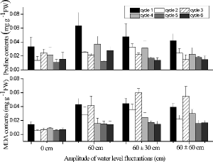
Figure8. Effects of four water-level fluctuation treatments (0 cm, 60 cm, 60 ± 30 cm, and 60 ± 60 cm) on chlorophyll a content in Acorus calamus. All the values are means of triplicates ± SD.

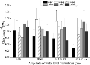
Figure9. The soluble sugar concentrations of shoot, rhizome, and root in Acorus calamus in four water-level fluctuation treatments (0 cm, 60 cm, 60 ± 30 cm, and 60 ± 60 cm). All the values were means of triplicates ± SD. Different letters within a graph indicate significant differences among treatments.

Discussion

Our data showed that biomass production and biomass allocation patterns differed significantly among the four water-level treatments. RGR and plant biomass were higher in the 60 ± 60 cm treatment than in the 60 ± 30 cm and 60 cm treatments. Negative growth rate occurred in the 60 cm treatment because plants were subjected to submergence. In this situation, they faced not only reduced gas exchange, but also altered light conditions which undoubtedly affected photosynthesis. However, when subjected to only periodic flooding in the 60 ± 60 cm treatment, biomass production was five times greater than that in the 60 cm treatment. Because underwater photosynthesis in emergent plants is usually limited by carbon dioxide availability, plants growing in the 60 ± 60 cm treatment were likely stressed during those weeks when water levels were 120 cm but compensated when water levels were at 0 cm. The maintenance of aerial biomass with depth may be critical for survival. Changes in the allocation of shoot biomass led to greater investment in below-ground biomass in the 60 ± 60 cm plants. This response probably allowed A. calamus to stretch towards the water surface at 120 cm and thus to maximize photosynthesis and survival.

The patterns in shoot morphology suggested that the growth of A. calamus was influenced by the WLFs. Next to the 0 cm control, the shoots of A. calamus grew the longest in the 60 ± 60 cm treatment but decreased in length in a near linear fashion in the 60 cm treatment, indicating a high degree of morphological plasticity. Water depth and shoot length appear to be intricately intertwined in aquatic plants in general, yet little is known about this relationship. In response to permanent increases in water depth, macrophytes undergo morphological adaptation, driven by elongation of the shoot or stem, to maintain a viable emergent canopy (Grace 1989; Blanch et al. 1999). Shoot elongation is the primary response to increasing water depth that enables them to emerge from the water in order to prevent carbon or light limitation of photosynthesis (Grace 1989). This is a characteristic of wetland plants such as Schoenoplectus species that are only able to grow to intermediate depths (Clevering & Hundschneid 1998). However, growth-mediated morphological adaptation, which results in a different set of traits to optimize resource capture, takes time to occur. However, WLFs can occur relatively quickly so that plants may not have the opportunity to morphologically adjust before water levels change once again (Vretare et al. 2001). In that situation, morphological adaptation will not occur and the plants will maintain an intermediate morphology. The time needed to morphologically adapt will depend on many factors, but as an example, the macrophyte Eleocharis cellulosa took 3 weeks to adjust morphological characters to new water-level conditions and 9 weeks to shift biomass partitioning (Edwards et al. 2003). The high frequency of cyclic fluctuations in our experiment (1 week) would likely preclude any morphological adaptation that might otherwise ameliorate the resource limitations caused by inundation (Zhang et al. 2013).

In this study, the root:shoot ratio was the highest in the 0 cm treatment and the roots were flooded but the shoots were exposed to air; thus, the plants allocated most biomass to below-ground organs, which can be interpreted as placement of resource-acquiring tissues (roots, rhizomes) in a resource-supplying environment (nutrients). This complemented the high availability of light and photosynthetic/respiratory gases (Rita 2005), leading to high photosynthetic rates. The rhizomes of A. calamus constituted a bigger proportion of the total below-ground biomass in the 60 ± 60 cm, 60 ± 30 cm, and 60 cm treatments compared to the 0 cm treatment. This relatively high proportion of rhizome could be due to the translocation of reserved resources from shoots more rapidly during the submergence period (Waters & Shay 1991; Lentz & Dunson 1998). Besides being subjected to extreme WLFs, the plants needed to support the relatively longer and bigger shoots and blades; the plant most likely developed bigger vertical rhizomes to sustain the plant body against disturbance (Waters & Shay 1991; Lentz & Dunson 1998). Results of the present study supported the important role of rhizome as a storage organ for Acorus plants (Haldemann & Brändle 1986, 1988; Weber & Brändle 1996), because it possesses both high biomass (Vojtíšková et al. 2004) and high carbohydrate storage capability in comparison to its roots.

A. calamus grown in the 60 cm, 60 ± 30 cm, and 60 ± 60 cm treatments were subjected to flooded conditions at least half of the time. The main stress to plants was the reduced oxygen supply, which made it possible for anaerobic respiration to occur in plants. In addition, the utilization efficiency of carbohydrate decreased and consumption of nutrients in vivo increased. Meanwhile, because of the reduction in light and carbon dioxide in the water column, the photosynthetic production of the macrophyte was seriously hindered (Voesenek et al. 2006). This led to a decrease in biomass and nutrient reserves of the plants subjected to long-term submergence (60 cm). In order to alleviate the damage of flooding, the plants could have employed different strategies to adapt to the water environment, such as accelerating the growth of branches and leaves to flee the flood stress (Panda et al. 2008), or growing slowly to reduce energy consumption, or relying on the amount of nutrient reserves under long-term flooding (Luo et al. 2007).

In our experiment, visible symptoms of injury caused by WLFs included yellowing of older leaves and slow or negative growth in roots and shoots in A. calamus. Some shoots of A. calamus were dead after 4 weeks in the 60 cm treatment, while no shoot death occurred in the 60 ± 60 cm treatment. Chlorophyll a concentrations of A. calamus responded negatively to WLFs but the response was not as varied as expected. Chlorophyll a concentrations of shoots decreased in the sixth cycle, mainly because of ethylene-induced chlorophyll degradation (Macek et al. 2006). Because ethylene can trigger gene expression and enzyme activity of chlorophyllase, it can reduce the potential for active CO₂ fixation.

MDA is a product of lipid peroxidation and an indicator of free radical production and consequent tissue damage. Its increase indicates that plants are under a high level of antioxidative stress (Hou et al. 2007). Our results showed that with the increasing amplitude of WLF, the MDA concentrations increased, which was similar to the effects of flooding on other higher plants (Sinha & Saxena 2006; Zhang et al. 2007). Under stress conditions such as drought, salinity, and extreme temperatures, proline may act as an osmotic adjustment mediator, a subcellular structure stabilizer, a free radical scavenger, and a redox potential buffer, and is an important component of cell wall proteins (Molinari et al. 2007). In our study, the 60 cm treatment was probably deep enough to provide a stressful environment for A. calamus (Cooper et al. 1996). WLFs induced variation in proline concentrations, suggesting that osmosis of membranes was affected by the stress caused by WLF, which was in accord with reports on other plants (Bassi & Sharma 1993; Sinha & Saxena 2006; Sinha et al. 2009).

The abundance of stored carbohydrates is connected with tolerance of wetland plant species to anoxia (Barclay & Crawford 1982, 1983). Large carbohydrate storage in tissue favors macrophytes that live longer in the absence of oxygen or in hypoxic conditions. A.calamus is one of the most anoxia-tolerant species (Crawford & Brändle 1996; Weber & Brändle 1996), and the rhizome is able to support its survival for more than 3 months in anoxic conditions (Crawford & Brändle 1996). In the study, the SS of plants was positively related to the amplitude of WLF.

A. calamus subjected to WLFs had different growth and morphological responses for responding to this change. In the 60 cm treatment, submergence had a negative effect on plant growth. But with fluctuating water levels, A. calamus was able to tolerate periods of major flooding for up to 12 weeks and even will be able to regrow above water level from depths of up to 120 cm. In summary, our results suggested that the distribution of A. calamus should be broadly tolerant, growing in areas with fluctuating water levels. Growth seems to be maximal in shallow water and the upper and lower depth limits are apparently related to flood and exposure tolerance. In addition, some physiological responses were found in A. calamus to different WLFs. Knowledge of how vegetation parameters, such as growth and morphological responses, proline and MDA concentrations in shoots, chlorophyll a concentrations and SS concentrations, are related to WLFs will be valuable in understanding and predicting the response of emergent vegetation to environmental management practices. Management decisions related to the conservation of this species should take into account possible disturbances to the hydrologic regime.

Acknowledgements

The authors would like to sincerely thank professor Zhang Yongyuan and Mohammad Russel for their comments and suggestions. The assistance of Wu juan, Ge Fangjie, Wei Hehong, Tang Haibin, and Zhu Guorong are also acknowledged.

Funding

This work was supported by Major Science and Technology Program for Water Pollution Control and Treatment [grant number 2009ZX07106-003], [grant number 2011ZX07303-001].

References

- Barclay AM, Crawford RMM. 1982. Plant-growth and survival under strict anaerobiosis. J Exp Bot. 33:541–549.
- Barclay AM, Crawford RMM. 1983. The effect of anaerobiosis on carbohydrate-levels in storage tissues of wetland plants. Ann Bot. 51:255–259.
- Bassi R, Sharma SS. 1993. Changes in proline content accompanying the uptake of zinc and copper by Lemna minor. Ann Bot. 72:151–154.
- Bates LS, Waldren RP, Teare ID. 1973. Rapid determination of free proline for water-stress studies. Plant Soil. 39:205–207.
- Blanch SJ, Ganf GG, Walker KF. 1999. Growth and resource allocation in response to flooding in the emergent sedge Bolboschoenus medianus. Aquatic Bot. 63:145–160.
- Blanch SJ, Walker KF, Ganf GG. 2000. Water regimes and littoral plants in four weir pools of the River Murray, Australia. Reg Rivers: Res Manage. 16:445–456.
- Boar RR, 2006. Responses of a fringing Cyperus papyrus L. swamp to changes in water level. Aquatic Bot. 84:85–92.
- Caicedo JR, Van der Steen NP, Arce O, Gijzen HJ. 2000. Effect of total ammonia nitrogen concentration and pH on growth rates of duckweed (Spirodela polyrrhiza). Water Res. 34:3829–3835.
- Casanova MT, Brock MA. 2000. How do depth, duration and frequency of flooding influence the establishment of wetland plant communities? Plant Ecol. 147:237–250.
- Clarke E, Baldwin AH. 2002. Responses of wetland plants to ammonia and water level. Ecol Eng. 18:257–264.
- Clevering OA, Hundschneid MPJ. 1998. Plastic and non-plastic variation in growth of newly established clones of Scirpus (Bolboschoenus) maritimus L. grown at different water depths. Aquatic Bot. 62:1–17.
- Cooling MP, Ganf GG, Walker KF. 2001. Leaf recruitment and elongation: an adaptive response to flooding in Villarsia reniformis. Aquatic Bot. 70:281–294.
- Cooper PF, Job GF, Green MB, Shutes RBE. 1996. Reed beds and constructed wetlands for wastewater treatment. Swindon, UK: Water Research Centre Publications; p. 154.
- Crawford RMM, Brändle R. 1996. Oxygen deprivation stress in a changing environment. J Exp Bot. 47:145–159.
- Deegan BM, White SD, Ganf GG. 2007. The influence of water level fluctuations on the growth of four emergent macrophyte species. Aquatic Bot. 86:309–315.
- Edwards AL, Lee DW, Richards JH. 2003. Responses to a fluctuating environment: effects of water depth on growth and biomass allocation in Eleocharis cellulosa Torr. (Cyperaceae). Can J Bot. 81:964–975.
- Grace JB. 1989. Effects of water depth on Typha latifolia and Typha domingensis. American J Bot. 76:762–768.
- Haldemann C, Brändle R. 1986. Seasonal-variations of reserves and of fermentation processes in wetland plant rhizomes at the natural site. Flora. 178:307–313.
- Haldemann C, Brändle R. 1988. Amino-acid composition in rhizomes of wetland species in their natural habitat and under anoxia. Flora. 180:407–411.
- Hou W, Chen X, Song G, Wang Q, Chang CC. 2007. Effect of copper and cadmium on heavy metal polluted water body restoration by duckweed (Lemna minor). Plant Physiol Biochem. 45:62–69.
- Kennedy MP, Milne JM, Murphy KJ, 2003. Experimental growth responses to groundwater level variation and competition in five British wetland plant species. Wetlands Ecol Manag. 11:383–396.
- Lentz K, Dunson WA. 1998. Water level affects growth of endangered northeastern bulrush, Scirpus ancistrochaetus Schuyler. Aquatic Bot. 60:213–219.
- Li H. 2000. Principles and techniques of plant physiological biochemical experiment. Beijing: Higher Education Press.
- Luo FL, Zeng B, Chen T, Ye XQ, Liu D. 2007. Response to simulated flooding of photosynthesis and growth of riparian plant Salix variegata in the Three Gorges reservoir region of China. Acta Phytoecologica Sinica. 31(5):910–918.
- Macek P, Rejmánková E, Houdková K. 2006. The effect of long-term submergence on functional properties of Eleocharis cellulosa Torr. Aquatic Bot. 84:251–258.
- Molinari HBC, Marur CJ, Daros E, de Campos MKF, de Carvalho J, Filho JCB, Pereira LFP, Vieira LGE. 2007. Evaluation of the stress-inducible production of proline in transgenic sugarcane (Saccharum sp.): osmotic adjustment, chlorophyll fluorescence and oxidative stress. Plant Physiol. 130:218–229.
- Nicol JM, Ganf GG, Pelton GA. 2003. Seed banks of a southern Australian wetland: the influence of water regime on the final floristic composition. Plant Ecol. 168:191–205.
- Panda D, Sharma SG, Sarkar RK. 2008. Chlorophyll fluorescence parameters, CO2 photosynthetic rate and regeneration capacity as a result of complete submergence and subsequent re-emergence in rice (Oryza sativa L.). Aquatic Bot. 88(2):127–133
- Porra RJ. 2002. The chequered history of the development and use of simultaneous equations for accurate determination of chlorophylls a and b. Photosynthesis Res. 73:149–156.
- Rea N, Ganf GG. 1994. The role of sexual reproduction and water regime in shaping the distribution patterns of clonal emergent aquatic plants. Aust Marine Freshwater Res. 45:1469–1479.
- Rita CH. 2005. Growth and biomass allocation in Scirpus littoralis Schrad. under different water depths. Bull Natl Inst Ecol. 15:153–160.
- Sarkar RK. 1998. Saccharide content and growth parameters in relation with flooding tolerance in rice. Biol Plant. 40:597–603.
- Sinha S, Basant A, Malik A, Singh KP. 2009. Iron-induced oxidative stress in a macrophyte: a chemometric approach. Ecotoxicol Environ Saf. 72:585–595.
- Sinha S, Saxena R. 2006. Effect of iron on lipid peroxidation, and enzymatic and non-enzymatic antioxidants and bacoside-A content in medicinal plant Bacopa monnieri L. Chemosphere. 62:1340–1350.
- Sorrell BK, Tanner CC. 2000. Convective gas flow and internal aeration in Eleocharis sphacelata in relation to water depth. J Ecol. 88:778–789.
- Squires L, van der Valk AG. 1992. Water-depth tolerances of the dominant emergent macrophytes of the Delta Marsh, Manitoba. Can J Bot. 70:1860–1867.
- Voesenek LACJ, Clomer TD, Pierik R, Millenaar FF. 2006. How plants cope with complete submergence. New Phytologist. 170(2):213–226.
- Vojtíšková L, Munzarová E, Votrubová O, Řihová A, Juřicová B. 2004. Growth and biomass allocation of sweet flag (Acorus calamus L.) under different nutrient conditions. Hydrobiologia. 518:9–22.
- Vretare V, Weisner S, Strand J A, Granél W. 2001. Phenotypic plasticity in Phragmites australis as a functional response to water depth. Aquatic Bot. 69:127–145.
- Wantzen KM, Rothhaupt K-O, Mörtl M, Cantonati M, G.-Tóth L, Fischer P, editors. 2008. Development in hydrobiology, Vol. 204: ecological effects of water-level fluctuations in lakes. The Netherlands: Springer; p. 21–31.
- Waters I, Shay JM. 1991. Effect of water depth on population parameters of a Typha glauca stand. Can J Bot. 70:349–351.
- Weber M, Brändle R. 1996. Some aspects of the extreme anoxia tolerance of the sweet flag, Acorus calamus L. Folia Geobot Phytotaxonica. 31:37–46.
- White SD, Ganf GG. 1998. The influence of convective flow on rhizome length in Typha domingensis over a water depth gradient. Aquatic Bot. 62:57–70.
- Zhang XZ, Liu XQ, Ding QZ. 2013. Morphological responses to water-level fluctuations of two submerged macrophytes, Myriophyllum spicatum and Hydrilla verticillata. J Plant Ecol. 6(1):64–70
- Zhang FQ, Wang YS, Lou ZP, Dong JD. 2007. Effect of heavy metal stress on antioxidative enzymes and lipid peroxidation in leaves and roots of two mangrove plant seedlings (Kandelia candel and Bruguiera gymnorrhiza). Chemosphere. 67:44–50.