Change in nutrient loading pattern due to coupled effect of change in concentration and hydroclimatic forces

ABSTRACT

Increase in nutrient loading into large riverine systems is of interest because of long-lasting negative effects on downstream water bodies. We know little of this phenomenon with respect to long-term relationships between water quality metrics and trends in river flow. Here we present a multi-decadal (1937–2014) examination of nutrient transport patterns of the South Saskatchewan and Red Deer Rivers, Canada. Using a multi-method approach, we show a slightly increasing trend in annual volume of water reaching a mid-watershed reservoir (Lake Diefenbaker) concomitant with a change in seasonal variability of flow events from the 1970s. Both total nitrogen (TN) and total phosphorus (TP) flux increased during the period of record. TN concentration increased, while TP concentration decreased. On average, the high-flow season transported 95% of annual TP flux, 75% of annual TN flux, and 65% of annual flow. Inter-annually, high-flow season contributions decreased with respect to water volume, but increased with respect to both TN and TP flux. We believe that changes in variability but also timing of hydroclimatic forces are responsible for observed patterns. Higher flows and more precipitation during the high-flow season are most likely responsible for increasing nutrient load regardless of overall decreases in nutrient concentration.

KEYWORDS:

• Nutrient transportation
• phosphorus
• nitrogen
• eutrophication
• climate change
• Lake Diefenbaker

Introduction

High levels of phosphorus (P) and nitrogen (N) can cause eutrophication, resulting in undesirable effects such as the dominance of toxin-producing cyanobacteria and reduction of dissolved oxygen concentrations in the hypolimnion of lakes and reservoirs (Schindler et al. 2008; Winder 2012). It is now evident that anthropogenic N and P inputs to aquatic systems have increased dramatically as a result of increased rainfall, atmospheric deposition, and agricultural activities (Chang et al. 2001; Hundey et al. 2016).

The magnitude, timing, and composition of storm-mediated discharge events can affect biogeochemical processes in water bodies (Vanni et al. 2006), but also proliferation of toxic cyanobacteria (e.g. Planktothrix rubescens) which appears when lake warming and higher N:P ratios occur simultaneously (Posch et al. 2012). We can confidently say that achieving current water quality objectives is likely to be more difficult as a result of the changes in hydrology and nutrient transport (IPCC 2007). Therefore, it is necessary that our key indicator variables of water quality are comprehensively analysed in the context of change in hydrological patterns.

Flux is a key variable in monitoring the quality of downstream receiving waters; however, concentration is the principal indicator for evaluating the overall functioning of a river reach being sampled (Hirsch et al. 2010). By definition, flux is the product of concentration and streamflow, which means that flux and concentration are closely related. However, the dynamics of concentration and flux can be considerably different from each other due to discharge variability which makes it difficult to evaluate the effectiveness of control strategies in a watershed. Despite progress in presenting trend data in nutrient concentrations and flux (Hirsch et al. 2010), there remain unanswered questions about the long-term variation of water quality of water bodies, and differences in N versus P transport, particularly in highly agricultural and regulated watersheds.

Long-term studies can provide insight into evaluating progress towards water quality objectives, anticipating where necessary actions need to be taken to prevent degradation of water resources, and developing effective remediation strategies (Dubrovsky et al. 2010). Here, we assess long-term patterns of total nitrogen (TN) and total phosphorus (TP) in terms of flux and concentration from the Red Deer River (RDR) and South Saskatchewan River (SSR), in western Canada. Our analysis is conducted on data obtained from the downstream stretch of tributaries immediately prior to their confluence upstream of a large reservoir, Lake Diefenbaker (LD). We principally examine: (1) the long-term nutrient transportation pattern entering LD and if it has changed over time; (2) the long-term relationship between flow, concentration, and flux; and (3) how any potential changes in the relationship of flow, concentration, and flux may affect the ecological state of the reservoir.

In our study, we intend to show how the coupled impact from changes in concentration (representative of anthropogenic stressors) and hydrological forces (streamflow and rainfall) influences the nutrient transportation patterns. To efficiently achieve this goal, we focused on a selected set of variables (TN and TP flux and concentration) that could be considered as indicators of the potential changes. We do not identify sources of TN and TP, and acknowledge that relative bioavailability of nutrient inputs is important. However, our focus here is on the implications of flux and concentration of TN and TP to receiving water bodies (where conversion processes lessen the importance of specific bioavailability of nutrient inputs at their upstream source).

To address our objectives, we employ comprehensive statistical and exploratory analyses to evaluate long-term relationships across several temporal scales. While nutrient loading is expected to increase as a result of increasing flow, rainfall, and nutrient concentration (Kleinman et al. 2006), how nutrient concentration and hydroclimatic forces interact to impact nutrient transportation pattern in the context of climate change has not yet been explored. For instance, overall decreases in nutrient concentration might be compromised by increases in rainfall and flow, or vice versa (Posch et al. 2012). We may predict that the long-term changes in nutrient loading are primarily governed by hydroclimatic forces rather than actual concentration because in pastoral areas, like our study area, the main contributors of nutrient influx are from non-point sources. We hypothesize that transportation of N (mostly dissolved) would be affected more than P (mostly particulate) because of significant differences in their biochemical properties and pathways. Unlike most long-term studies on nutrient transportation which are limited to annual comparisons, our data-set allowed us to go beyond annual comparisons to study ecological irregularities in the context of hydroclimate change over decades. Shifts in the timing of the hydrological and ecological events due to global climate change and human activities have an extremely important implication in ecosystems functioning (Elser et al. 2009; Sitters et al. 2015). Therefore, we investigated whether and how seasonal contributions of concentration, flux, and flow have been altered inter-annually to identify any irregularities in nutrient transportation which could potentially affect biogeochemical processes in the lake. Finally, due to the importance of nutrient stoichiometry in aquatic ecosystems, we examined the long-term change of N:P ratio which can have a potential effect on the ecological state of the large water bodies. To our knowledge, the role of recent extreme hydrological events in nutrient transportation pattern has not yet been explored interactively with nutrient concentration and flux in the Canadian Prairies.

Material and methods

Study area

South Saskatchewan River at Medicine Hat

The South Saskatchewan River Basin (SSRB) is one of the major river basins in western Canada which comprises four sub-basins of the Bow River, Oldman River, RDR, and SSR (Figure 1). The sum of flows of the Bow and Oldman Rivers make up the flow in the SSR near the city of Medicine Hat, Alberta. The mean annual flow of the SSR at Medicine Hat is 4,803,000 Cubic Decameters (dam³) which is significantly less than the mean natural flow at 7,002,000 dam³, mainly due to impacts from regulation and water use in the Bow and Oldman sub-basins (AMEC 2009). The SSR has been reported to have better water quality compared to the Bow or the Oldman Rivers, perhaps due to adequate flows even during low flow periods (North/South Consultants Inc. 2007). The SSR sub-basin is considered oligotrophic; however, both TP and TN concentrations do occasionally exceed expectations (North/South Consultants Inc. 2007).

Figure 1. The South Saskatchewan River Basin and the locations of hydrometric/water quality stations. The South Saskatchewan River stations are at Medicine Hat and the Red Deer River stations are at Bindloss.

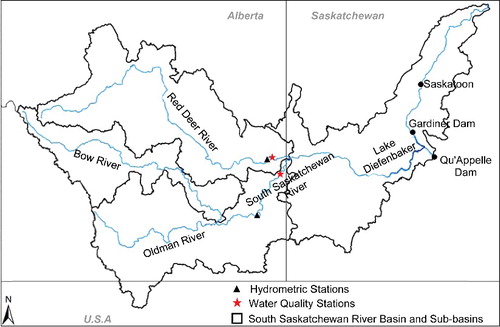
Red Deer River at Bindloss

The RDR originates in the Canadian Rocky Mountains and flows through a diverse landscape including mountainous areas, industrial lands, rangelands, irrigated farms, and urbanized areas making up its 44,683 km² drainage area. The RDR basin is the largest sub-basin of the SSRB by area; however, it contributes only about 20% to the annual flow of the SSR (Clipperton et al. 2003). The RDR has a mean discharge of 60 m³/s mainly from glacial run-off and snowmelt waters, with minor contributions from groundwater. Forestry, crop and livestock agriculture, petroleum and coal production, and recreation are considered the major economic activities of the basin (Hydroconsult EN3 Services Ltd 2002). The RDR catchment has been reported as stressed based on a six-year average of a Water Quality Index (WQI) values estimated from 2005 to 2010 (Saskatchewan Water Security Agency 2012). Our study locations were chosen because they could provide the best insight into examination of long-term water quality changes with respect to a downstream reservoir. These locations were best candidates because (Burke 2016): (1) Conversion of largely unaltered vegetated regions in the headwaters in SSRB to cropland and developed land downstream has resulted in accumulation of nutrient loading from anthropogenic sources to downstream; (2) a relatively higher proportion of those contributions are expected to come from the western tributaries regions

Lake Diefenbaker

LD was formed in 1969 by the construction of two earth-filled dams, the Gardiner and Qu'Appelle dams (Figure 1). LD is the largest reservoir along the SSR, and as a major source of drinking water, hydropower, irrigation, and recreation, it is the most economically important water body to the province of Saskatchewan. Average flow (1969–2014) into the reservoir was approximately 224 m³/s of which 98% was from the SSR. Although highly variable, the reservoir's water residence time is 1–3 years. Almost all nutrients and sediments are transported into LD from SSR (99%); while major export is through the Gardiner Dam (99%). Contributions of local run-offs to LD are typically insignificant, due to the region's soils, climate, and unusual hydrography (Shook and Pomeroy 2015). The limnology of the system is not yet well understood and there is concern regarding water quality deterioration due to its heavily agricultural watershed and climate variability.

Water quality and flow data

Since the late 1960s, Environment and Climate Change Canada has been monitoring water quality parameters at their Alberta/Saskatchewan border sites on SSR (AL05AK0001) and the RDR (AL05CK0001) in support of the Prairie Provinces Water Board. TP analytical methods were comparable over the period of record; however, TN analytical method was changed in 1993. Therefore, we analysed TN data once separately and then pooled together to determine if the final long-term trend was reasonably comparable. Flow data were obtained from Environment Canada's Water Survey of Canada (WSC) online database (http://www.wsc.ec.gc.ca). The two hydrometric stations in this study, 05AJ001 and 05CK004, have been operated by the WSC since 1911 and 1960, respectively (Table 1). Flow data were examined for the longest available flow record without missing days 1937–2014 for SSR and 1961–2014 for RDR. However, the focus of our analysis was on the periods of available water quality data where the relationships could be examined (Table 1). Due to insignificant hydrological contributions of RDR compared to SSR, the result from SSR is presented in more detail and is the basis of our conclusions. We also conducted our analyses on a temporal scale composed of two defined seasons, to determine seasonal differences in observed trends. We defined a ‘high-flow’ season (average of March, April, May, June, and July) and a ‘low-flow’ season (average of August, September, October, November, December, January, and February) to examine any potential inter-annual variations. This approach allowed us to identify the causative mechanisms properly because it is not as complex as monthly comparisons and not as generalized as yearly comparisons.

Table 1. Available data-set used for long-term nutrient transport study to Lake Diefenbaker, SK, Canada.

	South Saskatchewan River at Medicine Hat			Red Deer River at Bindloss
	Period of available data	Frequency of measurements	Station ID	Period of available data	Frequency of measurements	Station ID
TP concentration	1971–2014	Monthly	AL05AK0001	1974–2014	Monthly	AL05CK0001
TN concentration	1977–2014	Monthly	AL05AK0001	1977–2014	Monthly	AL05CK0001
Flow	1937–2014	Daily	05AJ001	1961–2014	Daily	05CK004

Statistical analysis

We examined both observed and estimated variables for the existence of trends at daily, monthly, and annual time scales, removing obvious outliers from our data-set. We adopted a multi-method approach to examine the consistency of results and to accurately detect the existence of any trends and regime shifts (see subsequent sections for detail descriptions of each method). Daily histories of concentration and flux were modelled using Weighted Regressions on Time, Discharge, and Season (WRTDS). Then, we used a non-parametric method, the Mann–Kendall (M-K) test, to detect any existing trends in streamflow, concentration, and flux series. We applied the Breaks for Additive Seasonal and Trend (BFAST) model to decompose any potential regime shifts of variables. We used histograms and heat maps to compare the frequency and the distribution of extreme values within each period identified by trend and seasonal break point (a point in time where the regime of the variable of interest is shifted based on significant change in the seasonality). As an empirical evidence of changes in hydrologic variability, we also examined the standard deviation of log-transformed daily flow to find out if changes have been happening in the overall variability of the flow record, regardless of whether the central tendency is changing over time. To determine if there was a significant change in the contribution of any months or seasons relative to the annual value, we divided the mean value of each individual month and season by the annual value. All tests were conducted in R (3.2.2 and higher versions), a statistical computing environment and language (https:/www.r-project.org/). The main packages used for the analyses were ‘EGRET’ and ‘EGRETci’ (Hirsch et al. 2015), ‘zyp’ (Bronaugh and Werner 2015) and ‘bfast’ (Verbesselt et al. 2015).

Weighted Regressions on Time, Discharge, and Season (WRTDS)

The WRTDS method uses weighted regressions to estimate concentration using time, discharge, and season as explanatory variables. The rationale for using weighted regression is to provide a better fit of observed data to the model because the coefficients can change over the domain of the data. The basic regression equation to estimate concentration iswhere c is concentration, in mg/L; β are the regression coefficients; q is ln(Q) where Q is daily mean discharge, in m³/s; T is time, in decimal years; and ϵ is the error (unexplained variation).

Hirsch et al. (2015) explain various desired features of WRTDS and its suitability for these types of studies. WRTDS is amenable for use with irregularly spaced samples with capability to detect temporal trends that may not follow a linear or quadratic functional form. In addition, it does not assume that the discharge versus concentration relationship has the same shape throughout the period of record, and that the concentration residuals are homoscedastic and seasonal pattern remains the same over the period of record. Finally, it provides not only estimates of the time series of annual mean concentrations and fluxes, but also time series of Flow Normalized Concentrations (FNC) and Fluxes (FNF) which integrate over the probability distribution of discharge to remove the effect of inter-annual streamflow variability.

WRTDS Bootstrap Test (WBT)

WBT is an extension of WRTDS that quantifies the uncertainty in WRTDS estimates of water quality trends. The results are presented as a likelihood-based approach as an alternative to the Null Hypothesis Significance Testing approach. The proposed terminology is partly based on language used by the Intergovernmental Panel on Climate Change (Mastrandrea and Mach 2011). A greater detail of the core mathematics and sensitivity analysis is described in Hirsch et al. (2010, 2015). Quality of the fitted model was evaluated using various diagnostic graphics (Appendix A; Supplemental data). We used the flux bias statistic here as a dimensionless representation of the difference between the sum of the estimated fluxes on all sampled days and the sum of the true fluxes on all sampled days. Overall, WRTDS is substantially less susceptible to serious flux bias; however, it is not immune to the problem (Moyer et al. 2012; Hirsch 2014). Because WBT only works with FNF and FNC series, trend identifications of the non-normalized and flow series were examined using BFAST (Table 2). The results from both methods were compared with the M-K trend test analysis which was conducted in more detail and various time scales to provide a reliable final interpretation and the relationships between the different series (Appendix B; Supplemental data).

Table 2. Identified trends in South Saskatchewan River and Red Deer River. WRT model only works with flow-normalized series; therefore, BFAST was used for examination of none flow-normalized series and flow series. A greater detail of the descriptive statements of trend likelihood are described in Hirsch et al. (2015).

		BFAST (on non-normalized series)				WBT (on flow-normalized series)
		Trend segments	β	p-value	Seasonal break point	Period of analysis	Change in FNC (mg/L) FNF (10^6 kg/yr)	p-value	Descriptive statements of trend likelihood
South Saskatchewan River	TP concentration	1971–2014	0.00	0.00	None	1971–2014	−0.03	0.04	Downward trend in concentration is highly likely
	TP flux	1971–2000	−0.01	0.13	1989	1971–2014	0.32	0.65	Upward trend in flux is likely
		2001–2014	0.08	0.00
	TN concentration	1977–2002	−0.01	0.00	None	1977–1993	−0.25	0.02	Downward trend in concentration is highly likely
		2003–2014	0.01	0.02		1994–2014	0.17	0.09	Upward trend in concentration is highly likely
	TN flux	1977–2000	0.02	0.01	None	1977–1993	−0.71	0.10	Downward trend in flux is highly likely
		2001–2014	0.09	0.00		1994–2014	1.46	0.23	Upward trend in flux is likely
	Flow 1937-2014	1937–1954	0.05	0.00	1975
		1955–1981	−0.01	0.01
		1982–1994	0.05	0.00
		1995–2014	0.05	0.00
	Flow 1975-2014	1975–1994	0.04	0.00	None
		1995–2014	0.01	0.29
Red Deer River	TP concentration	1974–2000	0.00	0.30	None	1974–2014	−0.01	0.94	Downward trend in concentration is about as likely as not
		2001–2014	0.06	0.00
	TP flux	1974–2000	0.02	0.01	None	1974–2014	0.00	0.84	Downward trend in flux is about as likely as not
		2001–2014	0.10	0.00
	TN concentration	1977–1989	−0.05	0.00	None	1977–1993	−0.58	0.02	Downward trend in concentration is highly likely
		1990–2014	0.03	0.00		1994–2014	0.47	0.03	Upward trend in concentration is highly likely
	TN flux	1977–2000	0.02	0.01	None	1977–1993	−1.41	0.02	Downward trend in flux is highly likely
		2001–2014	0.09	0.00		1994–2014	1.69	0.07	Upward trend in flux is highly likely
	Flow 1961-2014	1961–2000	0.01	0.00	1983
		2001–2014	0.04	0.00
	Flow 1974-2014	1974–1998	0.02	0.08	None
		1999–2014	0.04	0.00

Note: TP, total phosphorus; TN, total nitrogen; BFAST, Breaks for Additive Seasonal and Trend; WRT, Weighted Regressions on Time; WBT, WRTDS bootstrap test; FNC, flow-normalized concentration; FNF, flow-normalized flux.

Mann–Kendall trend analysis

The M-K test is a non-parametric method, which does not require normal distribution of data. However, the M-K test is sensitive to serial correlation in time series data which will affect the ability of the test to assess the significance of trends (Von Storch and Zwiers 1999). Our data exhibited significant autocorrelation which we were required to address prior to any trend analysis. In order to remove the existing autocorrelation component of the time series, we applied the Trend-Free Pre-Whitening technique, as proposed by Yue et al. (2002, 2003).

Time series decomposition

BFAST integrates the iterative decomposition of time series into trend, seasonal, and remainder components for examining changes within time series. BFAST iteratively estimates the time and number of changes, and characterizes change by its magnitude and direction (Verbesselt, Hyndman, Newnham, and Culvenor 2010). BFAST can be used to analyse different types of data dealing with seasonal or non-seasonal time series, such as hydrology and climatology with capability to identify the regime shift (Zhao et al. 2015). A more complete description can be found from Verbesselt, Hyndman, Zeileis, and Culvenor (2010).

Results

Flow

SSR mean flow for 1937–2014 was 180 m³/s; however, the mean for 1971–2014 was 164 m³/s. RDR mean flow for 1961–2014 was 58.5 m³/s, while the mean for 1974–2014 was slightly lower at 56.9 m³/s. SSR annual flow volume ranged from a low of approximately 1.7 million dam³ in 2001 to a high of approximately 13.2 million dam³ in 1951.

The SSR long-term hydrograph indicates that the rising limb starts to develop rapidly at mid-March resulting in peak flows occurring mostly in June and sometimes in July (Figure 2). Flow begins to decrease rapidly in early July with occasional small peaks during August and September (Figure 2). Unlike SSR, the high-flow season of RDR extends from early March to late August with two major rising limbs. Highest flows occur in April and June with an occasional small peak in late September. Figure 3 illustrates different components of SSR monthly flow from 1937 to 2014 decomposed by BFAST. The log-transformed series is shown in Figure 3(a) while Figure 3(b,c) display the estimated seasonal and trend components, respectively. The remainder noise is shown in Figure 3(d). When the analysis was done for 1937–2014, we identified a regime shift at around 1975 in the fitted seasonal component (Figure 3(b)). In addition, the fitted trend component (Figure 3(c)) identified three trend break points. A significant increase (P = 0.001) was detected from 1937 to 1954, followed by a decreasing trend from 1955 to 1981. Finally, the third (1982–1994) and fourth period (1995–2014) both showed significant increasing trends. Because the water quality data were available only from early 1970s onward and the flow regime was shifted at around 1975, a separate decomposition analysis was conducted for 1975 to 2014 SSR flow series. In this case, no seasonal break point was identified, while flow increased during both 1975–1994 (P = 0.001) and 1995–2014 (P = 0.285) periods. Flows of higher than 180 m³/s have been occurring significantly more during 1995-–2014 (Figure 4). Time series decomposition of RDR monthly flow identified one seasonal break point around 1983 and one trend break point at 2000. Trends of both before and after 2000 were significantly upward; however, 2000–2014 had a greater slope than 1961–2000.

Figure 2. The long-term hydrograph of SSR (left) and RDR (right). For both tributaries, the data were divided into two separate series of ‘before and after’ the identified regime shift, which was at around 1975 and 1983 for SSR and RDR, respectively.

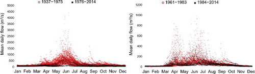
Figure 3. Monthly streamflow decomposition of the SSR at Medicine Hat station. Log-transformed flow data were used to stabilize the variances.

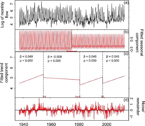
Figure 4. Histograms of SSR daily flows for the earlier and most recent periods after the identified regime shift at around 1975.

Inter-annual M-K trend test on SSR mean flow during 1937–2014 indicated decreasing trends for April, May, June, July, August, annual mean and high-flow season with only April and May being statistically significant (Appendix B). The contribution of high-flow season for SSR has decreased (P = 0.02), while the low-flow season contribution has increased (P = 0.02) from 1937 to 2014. When the M-K monthly analysis was only conducted for 1971–2014, the result was relatively different and more indicative of increasing trends. In this case, June, July, August, annual mean and high-flow season had increasing trends (statistically non-significant). Our M-K trend test on RDR flow for 1974–2014 indicated that annual mean flow has been increasing (P = 0.02). With respect to the standard deviation of log-transformed daily flow, an upward trend is apparent for the high-flow season of SSR from late 1960s (Figure 5(a)). SSR low-flow season has followed almost the same pattern as high-flow season until mid-1980s when it declines (Figure 5(b)). A horizontal line indicates that all quantiles of the distribution had increased by the same percentage amount; however, an upward slope is indicative of a greater percentage change in the high end and/or low end of the distribution, compared to the percentage change in the middle portion of the distribution. For RDR, the standard deviation of log-transformed daily flow of both seasons showed a significant downward slope until late 1980s.

Figure 5. Plots of the standard deviation of log-transformed flow over time, SSR at Medicine Hat. (a) High flow-season, (b) low-flow season, and (c) the entire year. The vertical axis represents the standard deviation of the logged flow which is dimensionless and a measure of relative variability.

Total phosphorus concentration and flux

Using WRTDS, we estimated the long-term TP concentration and flux for both SSR (1971–2014) and RDR (1974–2014). Figure 6 shows the long-term monthly average TP concentration and flux for both tributaries. The long-term average concentrations for SSR and RDR were 0.082 and 0.133 mg/L, respectively. Monthly averages show that June had the highest concentration in both SSR (0.287 mg/L) and RDR (0.302 mg/L). However, October (0.027 mg/L) and January (0.020 mg/L) had the lowest concentrations in SSR and RDR, respectively. The average annual TP flux for SSR and RDR was 1444 tons/year and 598 tons/year, respectively. June had the highest contribution to the annual TP transport in both tributaries with 58% (SSR) and 26% (RDR). For SSR, the highest and lowest annual TP flux belonged to 2013 and 2001 with 7823 and 65 tons, respectively (Figure 8). However, for RDR, the highest and lowest annual TP flux belonged to 2007 and 1984 with 1787 tons and 111 tons, respectively.

Figure 6. Long-term monthly flux and concentration estimated using WRTDS for SSR at Medicine Hat and RDR at Bindloss.

The M-K trend test indicated a significant decreasing trend for both non-normalized annual (P = 0.04) and flow-normalized (P = 0.001) TP concentration of SSR. The majority of months showed a similar decreasing trend in concentration, except months of June, July, and August (Appendix B). With respect to non-normalized flux, both annual mean and high-flow season showed slightly increasing trends (Appendix B). However, low-flow season TP flux has been decreasing significantly (P = 0.002). Regarding the seasonal contribution to the annual TP flux, high-flow season and low-flow season contributions have been non-significantly (P = 0.21) increasing and decreasing, respectively.

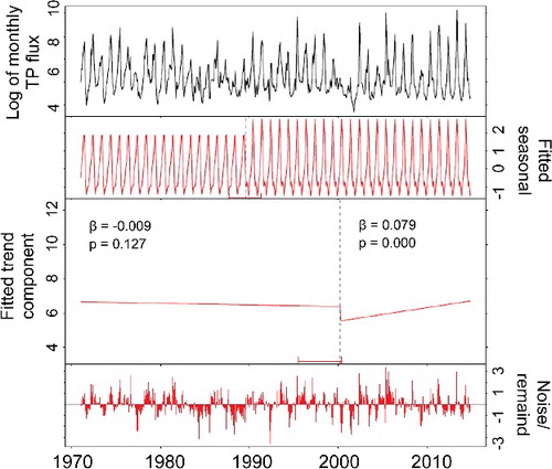
Time series decomposition of SSR monthly TP concentration identified neither a seasonal break point nor a trend break-point, but a steady decreasing trend for the entire period of record (P = 0.001). However, a seasonal break point was identified for SSR monthly TP flux around 1989 and one major trend break point around 2000 (Figure 7) indicating a non-significant decrease (P = 0.127) during 1971–2000, but significant increase afterward (P = 0.001). For RDR, non-normalized concentration of all months (except March) showed signs of increase with June, November, and December being statistically significant (Appendix B). With respect to non-normalized flux for RDR, both annual and high-flow season have been significantly increasing (Appendix B). For RDR, one trend break point was detected within the concentration series at around 2000 with a non-significant decrease until 2000, but a significant increase afterward. Similarly, for TP flux we identified a trend break point at around 2000 with both before and after (relatively greater increase) periods increasing.

Figure 7. Trend decomposition of monthly TP flux for SSR at Medicine Hat station. Log-transformed flux data were used to stabilize the variances.

Total nitrogen concentration and flux

Overall, TN concentration of SSR (0.95 mg/L) was slightly higher than RDR (0.92 mg/L). Figure 6 shows the long-term monthly TN concentration and flux for SSR and RDR. Monthly averages show a noticeable difference in seasonality between two tributaries, with February having the highest concentration for SSR (1.587 mg/L), while April being the highest for RDR (1.953 mg/L). In addition, August (0.364 mg/L) and November (0.471 mg/L) had the lowest concentrations in SSR and RDR, respectively. The average annual flux for SSR and RDR were 6900 tons/year and 3135 tons/year, respectively. For SSR, month of June contributed the most with 36% of the TN annual flux, while for RDR it was during the month of April (24%). The highest and lowest annual TN flux of SSR belonged to 2005 and 2001 with 22,326 tons and 1520 tons, respectively. However, for RDR, the highest and lowest annual TN flux belonged to 2011 and 1988 with 9271 tons and 652 tons, respectively.

For SSR, during 1977–1993, the non-normalized annual concentration of TN decreased significantly. However, TN concentration has increased substantially from 1994 to 2014. Regarding the individual months during both periods, the trends were relatively similar to the annual concentration in terms of direction (Appendix B). With regard to TN flux, identifying a single trend over the entire period of record was more challenging due to the change in analytical method in 1993. Overall, the SSR result suggests that TN flux slightly decreased during 1977–1993, but started to increase afterward. Time series decomposition of SSR monthly non-normalized concentration identified no seasonal break point, but one trend break point (Table 2). The result showed that the concentration was significantly decreasing until around 2002, but it started to increase significantly afterward. For RDR, mean annual non-normalized TN concentration and flux were decreasing during 1977–1993, but started to increase significantly (P = 0.002 and 0.035) during 1994–2014 (Appendix B). In both tributaries, TN flux contribution of the high-flow season has increased which means that the low-flow season has been contributing less (Appendix B).

Discussion

Change in flux pattern: flow or concentration?

Our analysis shows that nutrient concentration, flux, and flow in our system have undertaken gradual changes but also a few abrupt changes through time. These changes were observable not only in terms of quantity, but also the pattern, frequency, and the distribution of high and low values. It is expected that the hydrologic regime of LD will be changed due to warming climate (Pomeroy et al. 2009; Vogt et al. 2015; Hudson and Vandergucht 2015). The extended trend from 1937 to 2014 is more suggestive of decreasing trend, also supported by other studies (Pomeroy et al. 2005; St. Jacques et al. 2013).

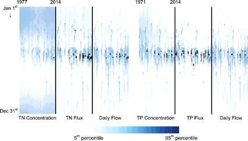
Since 1937, the SSR has experienced three periods of increasing flow that are most evident after 1975. Flow pattern during 1975–1994 can be distinguished from the preceding and succeeding periods by higher occurrence of low flows and less frequent high flows. As a result, during 1975–1994, both non-normalized concentration and flux were to some extent influenced negatively (Figure 8). In contrast, during 1995–2014, extreme high flows occurred more often relative to 1975–1994 (Figure 4), but here both non-normalized concentration and flux were positively influenced which leaded to a period of high nutrient transportation (Figure 8). The daily heat map of concentration, flux, and flow illustrates how the frequency of extremely high values has increased during the period of record (Figure 9). In addition, days with higher concentration, flux, and flow have gradually moved towards the month of June which is in concert with the result from Dumanski et al. (2015) for monthly rainfall on Smith Creek Research Basin (near the Saskatchewan–Manitoba border, east of our study area). Most likely, the increasing trend of TN concentration (since 1994) of both tributaries is due to anthropogenic stressors (land-use, urbanization, air pollution, wastewater effluent and agriculture) rather than hydrological stressors. This was supported by increasing trends of FNC of TN in both locations because the influence of flow is removed from the series. Similar to our findings, a recent study (Burke 2016) suggested that increasing trends of TN within several tributaries of the SSRB are from anthropogenic sources such as wastewater effluent that contributes various forms of nitrogen.

Figure 8. Annual flow, flux, and concentration series for the South Saskatchewan River at Medicine Hat.

Figure 9. A heat map created from daily concentration, flux, and flow of the South Saskatchewan River for the period of study. Both concentration and flux series are non-normalized values. Black bordered cells are values which are eight times higher than long-term mean for each variable as representation of extreme high flows, concentrations, and fluxes.

Seasonal or inter-annual variations in flow concomitant with the climate of the basin may explain the temporal variations of flux trends; however, concentration and flow may not exhibit the same variability which can result in flux and concentration having trends of different directions. For instance, concentrations of dissolved constituents are usually high during low-flow conditions, but diluted during high-flow seasons (Chang 2008), which was the case for the concentration of TN at SSR and to less extent at RDR (Figure 6). Further, some constituents (e.g. TP) can exhibit a pattern influenced by both dilution and run-off at the same time. A portion of TP may come from point sources such as sewage treatment plants (dilution effect), but another portion may be derived from surface run-off and be attached to sediment particles. The resulting pattern is an initial dilution, followed by a stronger increase with flow due to wash-off (Helsel and Hirsch 2002). Additional analyses (not presented here) showed that the ratio of total dissolved phosphorus (TDP)/TP in terms of both concentration and flux has been decreasing over time mostly due to increase in particulate phosphorus (PP). Similarly, but less significantly, the ratio of total dissolved nitrogen (TDN)/TN concentration has been decreasing over time mostly due to increase in particulate nitrogen (PN). This shows the importance of surface run-off from highly cultivated river basins during years with high flow events which have been the case from 1994 to 2014 in our study.

The overall increase of 21% (0.009 mg TN/L/year) and 64% (0.024 mg TN/L/year) during 1994–2014 at SSR and RDR, respectively, are quite alarming for downstream water bodies such as LD. Due to the coupled effect of increasing TN concentration and flow, we can see that FNF of TN was increasing even at a higher rate with an increase of 23% (80 tons TN/year/year) and 77% (100 tons TN/year/year) at SSR and RDR, respectively. Analysis of only annual means can be misleading for revealing the actual trend and causative mechanisms. For example, overall, the analyses have proved that TP concentration has decreased significantly for SSR. However, the long-term daily heat map (Figure 9) and monthly M-K test showed that TP concentrations have increased during the month of June when the largest amount of TP is transported within the system. In other words, the overall conclusion of decreasing TP concentration is mostly due to decreasing trends from September to May (nine months). We believe this difference in trend between months is most likely caused by higher flows and more rainfall events which have been more frequent during the high-flow season of the recent period. Such change in flow and rainfall pattern has most likely increased nutrient release through surface wash-off processes.

Although TN is mostly made of dissolved forms and the effect of high-flow events is expected to be different from TP (mostly particulate forms), we still can see similar effects on TN concentration and consequently flux during the month of June. The inter-annual variation of individual months for TN concentration is not as evident as TP because the effect of high flow events on TN is somewhat offset by the dilution effect. However, we still can see that high TN flux events have increased substantially, moderately due to higher concentration and mostly because of high flow events (Figure 9).

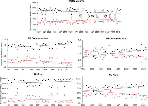
The result from SSR flow analysis suggests that the high-flow season contribution to the annual volume has decreased for the period of record which means that the low-flow season contribution has increased in the same rate (Figure 10). We can see that after 1975, the variability of the seasonal contribution has slightly increased. On average, high-flow season contributed 71% to the annual discharge during 1937–1975, while that was only 62% during 1976–2014. It would be expected to see a similar pattern for flux in terms of season's contribution; however, it was evident that the contribution of high-flow season for both flux and concentration has increased over time (Figure 10). This contradiction between flow and flux suggests the existence of other causative mechanisms in addition to the increasing annual flow during the period of water quality study.

Figure 10. The relative contribution of both high-flow and low-flow season to the annual mean for each variable in the South Saskatchewan River, Medicine Hat. The solid lines are linear-trend lines for each series. High-flow season series are shown in black; low-flow season series in red.

One possible explanation for the observed anomaly between flow and flux may lie in the earlier occurrence of high-flow events during the high flow season; however, we found no evidence for this. Because precipitation and run-off are the primary forces governing nutrient transport on the basin, we believe that examining the potential changes in precipitation and run-off pattern could better explain the difference between flow and flux in terms of their seasonal contribution. Dumanski et al. (2015) found that from 1942 to 2014 (in the Smith Creek Research Basin, Saskatchewan, approximately 200 km east of LD), annual rainfall has significantly increased at a rate of 0.9 mm/year, along with a 50% increase in the number of multiple-day events. They concluded that increases in rainfall (primarily in May and June) and frequency of multiple-day rainfall events in the summer months have evidently transformed snowmelt-dominated to rainfall-dominated run-off at the basin scale. We also examined daily precipitation data (Alberta Climate Information Service 2016) during 1961–2014 for upstream area (Calgary) in order to see if there have been any changes in precipitation pattern. The daily precipitation data during the high-flow season showed that the total number of rainy days and mean precipitation started to increase after 1980 (Figure 11). In addition, our M-K test indicated that high-flow season precipitation has been increasing at a rate of 0.006 mm/year along with a significant increase in the number of rainy days at a rate of 0.5 day/year (Figure 11(a,b)). These relationships suggest that TP and TN transport have been sustainably affected in both very dry and very wet years. This can be seen for two periods with relatively low flow contributions during high-flow seasons (1987–1989 and 2000–2002), resulting in relatively low concentration and flux (Figure 10). In contrast, consecutive wet years with relatively high contribution of flow during high-flow season (1994–1998 and 2010–2014) experienced relatively high concentration and flux for both TN and TP. For RDR, the seasonal contribution has almost stayed the same for all variables inter-annually.

Figure 11. (a) Mean precipitation during the high-flow season period, (b) number of rainy days for the season. Dashed lines are the four-year period moving average. Data were obtained from the Interpolated Weather Data Since 1961 for Alberta Townships by the Alberta Climate Information Service for the Calgary area.

The potential long-term biological imbalance on receiving water bodies

The interactions between nutrient concentration, flux, and flow are very complex which requires a careful evaluation of each variable relative to one another. It has been suggested that cross-ecosystem material flows spatially link ecosystems and influence food web dynamics (e.g. Sitters et al. 2015; McLoughlin et al. 2016). Changes in nutrient transport regime can alter the ratios of elements like carbon, nitrogen, and phosphorus which eventually impact food web interactions through stoichiometric mismatches between resources and consumers. In their literature review, Sitters et al. (2015) evaluated the importance of ecological stoichiometry and its usefulness for assessing the impact of cross-ecosystem materials on recipient ecosystems and organisms as it provides predicted responses to resource elemental ratios (Sterner and Elser 2002; Allen and Gillooly 2009).

Based on our analyses, overall decreases in TP concentration for the SSR have been compromised likely due to impacts from hydroclimatic factors (e.g. soil moisture, shifting precipitation regimes, evapotranspiration rates, and change in run-off regime). This was even more pronounced for TN due to the overall increase of concentration over the past two decades. Despite effective nutrient management and partial recovery of many lakes from phosphorus pollution, new research is suggesting that climate warming can bring the same problems back by changes in hydroclimatic forces and N:P ratio (Winder 2012). Yuan et al. (2014) found that Lake Erie's biological productivity has remained relatively high after transition from an oligotrophic state to a eutrophic state, even though nutrient control programmes were successfully implemented after the transitional phase. Based on climate change projections of reduced flow (Tanzeeba and Gan 2012), improvements in light conditions and reduced particulate nutrient loading are expected. However, bioavailable (dissolved) nutrient concentrations would either stay unchanged or potentially increase (Joosse and Baker 2011) which along with reduced volume of water and higher temperature could create a suitable environment for future algal blooms. Phytoplankton biomass in LD is highly influenced by availability of light which itself is affected by SSR flow, the composition of particulate matter and suspended sediments, wind pattern, stratification regime, mixing dynamics, and reservoir residence times (Dubourg et al. 2015).

During 2011 and 2012, cyanobacteria only contributed <5% of the total phytoplankton biomass most likely due to relatively short residence time (0.72 years in 2011 and 0.99 years in 2012) from the high flow events (Roelke and Pierce 2011; Abirhire et al. 2015). It has been shown that occurrence of drought conditions (low inflow and flushing rate) after high nutrient loads from high flow events can promote cyanobacterial blooms in lakes and reservoirs (Paerl and Huisman 2009). This is supported by observed cyanobacterial blooms in LD during years with low flow conditions (SEPS & EC 1988; Hecker et al. 2012; Hudson and Vandergucht 2015).

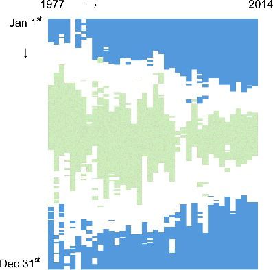
With regard to LD, these kinds of changes can have significant impacts on its water quality. The short-term impacts can be more as a result of change in nutrient concentration and flow entering the lake during warm season and consequent change in N:P ratio. We evaluated the long-term stoichiometric change of incoming flow with reference to the strict N (20) and P (50) deficiency thresholds (Guildford and Hecky 2000). The result from SSR (Figure 12) suggests that the TN:TP molar ratio has been substantially increasing with more days being within the P-deficient range (TN:TP > 50). This was consistent with the result of the physiological assays and compositional nutrient status indicators, suggesting P as the major limiting nutrient of phytoplankton in LD (Dubourg et al. 2015). In addition, there was a significant change regarding seasonal pattern with expansion of P-deficient days towards high-flow season, but shrinkage of N-deficient days (Figure 12). It has been suggested that proliferation of toxic cyanobacterial species is stimulated by a favourable condition that appears when lake warming and higher N:P ratios occur simultaneously (Posch et al. 2012).

Figure 12. Daily TN:TP molar ratio during 1977–2014 for the South Saskatchewan River at Medicine Hat. Blue indicates days with TN:TP ≥ 50 as strict P-deficiency, while green represents days with TN:TP ≤ 20 as strict N-deficiency (from Guildford and Hecky 2000). The white area represents any value >20 and <50.

Such disproportionate increases of TN in comparison to TP along with warmer water temperature might potentially shift the phytoplankton community in LD to the toxic cyanobacterial species promoted as suggested by Posch et al. (2012). Considering the placement of the reservoirs within nutrient-rich watersheds and their open characteristics, future changes in reservoir nutrient budget may significantly alter nutrient export to downstream water bodies in part because nutrients cannot indefinitely accumulate within bottom sediments (Powers et al. 2015). Even if we can manipulate the affected water bodies hydrologically and biologically, yet stricter nutrient management will likely be the most reasonable and efficient approach to long-term control of cyanobacteria in the face of more extreme hydroclimate forces (Paerl and Paul 2012).

Conclusions

We showed a slightly increasing trend in annual volume of water reaching LD concomitant with a change in seasonal variability of flow events during the period of water quality study (1970s to 2014). The substantial increase of TN and TP influx to LD is primarily because of hydroclimatic forces (e.g. extreme flows and precipitation pattern) rather than the actual nutrient concentration. It is evident that overall decreases in TP concentration are compromised by an increasing frequency of high flow events, directly enhancing nutrient transport from non-point sources. This is even more pronounced for TN due to coupled effect of increasing concentration along with higher flows.

We demonstrate that despite a strong, positive relationship between flow and flux, their seasonal contribution to the annual budget can be of dissimilar direction. The contribution of high-flow season with respect to water volume has been decreasing, while increasing with respect to influx of TN and TP. This important finding proves how the change in timing and frequency of extreme flows can alter the seasonality of nutrient transportation, composition, and the stoichiometry of the incoming flow to LD.

It is expected that biochemical composition of the sediment will change over time. This can eventually alter N and P cycles in the hypolimnion of LD which is in direct contact with the biggest store of N and P in the reservoir. If the high-flow season continues to bring nutrients to the reservoir at current increasing rates along with potentially lower water volume, prolonged stratification, and warmer water temperature, then we could expect to see higher occurrence of algal blooms in future. Moreover, disproportionate increase of TN relative to TP is suggestive of inefficient pollution control for nitrogen. This might potentially affect the phytoplankton community though stoichiometric change.

We believe that it is unlikely that a single climate or watershed management component is responsible for the dramatic shift in nutrient transportation pattern that we observed, but a combination of changing climate and land use practices. We believe that extensive restoration plans with emphasis on one component for reducing nutrient concentration may gradually be compromised by the effects of climate change.

Few prior studies have provided joint views on the variation in hydrology, nutrient concentration, and flux especially over periods >2 decades. Further investigation is recommended for constructing a long-term nutrient export study from LD to fully understand if the combination of stressors has affected nutrient retention rates of the reservoir.

Acknowledgments

We thank Environment and Climate Change Canada (Freshwater Water Quality Monitoring and Surveillance) for providing access to the data; and the Limnology Lab, University of Saskatchewan, for helping initiate this work. We also thank the reviewers for offering thoughtful comments and suggestions to improve the manuscript.

Disclosure statement

No potential conflict of interest was reported by the authors.

Additional information

Funding

This work was supported by scholarship and faculty funding from the Biology Department, University of Saskatchewan.

Notes on contributors

Farshad Shafiei

Farshad Shafiei is a PhD candidate at Department of Biology, University of Saskatchewan. He obtained and worked up data, and wrote the drafts of the manuscript.

Philip D. McLoughlin

Philip D. McLoughlin is a professor of Ecology, at the Department of Biology, University of Saskatchewan. He provided useful ideas and proof-read the drafts of the manuscript.

References

- Abirhire O, North RL, Hunter K, Vandergucht D, Sereda J, Hudson J. 2015. Environmental factors influencing phytoplankton communities in Lake Diefenbaker, Saskatchewan, Canada. J Gt Lakes Res. 41(Suppl 2):118–128.
- Alberta Climate Information Service. 2016. Interpolated weather data since 1961 for Alberta townships. [accessed 2016 Jan 6]. http://agriculture.alberta.ca/acis/township-data-viewer.jsp.
- Allen AP, Gillooly JF. 2009. Towards an integration of ecological stoichiometry and the metabolic theory of ecology to better understand nutrient cycling. Ecol Lett. 12:369–384.
- AMEC. 2009. South Saskatchewan river basin in Alberta: water supply study. Lethbridge (AB): Alberta Agriculture and Rural Development.
- Bronaugh D, Werner A. 2015. zyp: Zhang + Yue-Pilon trends package. Version 0.10-1. https://CRAN.R-project.org/package=zyp.
- Burke A. 2016. Water quality and nutrient load in the South Saskatchewan River basin, SK, Canada [master's thesis]. Saskatoon: (SK): University of Saskatchewan.
- Chang H. 2008. Spatial analysis of water quality trends in the Han River basin, South Korea. Water Res.. 42:3285–3304.
- Chang H, Evans BM, Easterling DR. 2001. The effects of climate change on streamflow and nutrient loading. J Am Water Resour Assoc. 37:973–985.
- Clipperton GK, Koning CW, Locke AGH, Mahoney JM, Quazi B. 2003. Instream flow needs determinations for the South Saskatchewan River basin, Alberta, Canada. Calgary (AB): Alberta Environment and Alberta Sustainable Resource Development. Pub No.: T/719.
- Dubourg P, North RL, Hunter K, Vandergucht D, Abirhire O, Silsbe GM, Guildford SJ, Hudson J. 2015. Light and nutrient co-limitation of phytoplankton communities in a large reservoir: Lake Diefenbaker, Saskatchewan, Canada. J Gt Lakes Res. 41(Suppl 2):129–143.
- Dubrovsky NM, Burow KR, Clark GM, Gronberg JM, Hamilton PA, Hitt KJ, Mueller DK, Munn MD, Nolan BT, Puckett LJ, et al. 2010. The quality of our nation's waters – nutrients in the nation's streams and groundwater, 1992–2004. Reston (VA): US Geological Survey Circular 1350. http://water.usgs.gov/nawqa/nutrients/pubs/circ1350.
- Dumanski S, Pomeroy JW, Westbrook CJ. 2015. Hydrological regime changes in a Canadian Prairie basin. Hydrol Process. 29:3893–3904.
- Elser JJ, Andersen T, Baron JS, Bergström AK, Jansson M, Kyle M, Nydick KR, Steger L, Hessen DO. 2009. Shifts in lake N: P stoichiometry and nutrient limitation driven by atmospheric nitrogen deposition. Science. 326:835–837.
- Guildford SJ, Hecky RE. 2000. Total nitrogen, total phosphorus, and nutrient limitation in lakes and oceans: is there a common relationship? Limnol Oceanogr. 45:1213–1223.
- Hecker M, Khim JS, Giesy JP, Li S-Q, Ryu J-H. 2012. Seasonal dynamics of nutrient loading and chlorophyll A in a Northern prairies reservoir, Saskatchewan, Canada. J Water Resour Prot. 4:180–202.
- Helsel DR, Hirsch RM. 2002. Statistical methods in water resources techniques of water resources investigations. Book 4, Chapter A3. U.S. Geological Survey. http://water.usgs.gov/pubs/twri/twri4a3/
- Hirsch RM. 2014. Large biases in regression-based constituent flux estimates: causes and diagnostic tools. J Am Water Resour Assoc. 50:1401–1424.
- Hirsch RM, Archfield SA, De Cicco LA. 2015. A bootstrap method for estimating uncertainty of water quality trends. Environ Model Softw. 73:148–166.
- Hirsch RM, Moyer DL, Archfield SA. 2010. Weighted regressions on time, discharge, and season (WRTDS), with an application to Chesapeake Bay River inputs. J Am Water Resour Assoc. 46:857–880.
- Hudson J, Vandergucht D. 2015. Spatial and temporal patterns in physical properties and dissolved oxygen in Lake Diefenbaker, a large reservoir on the Canadian Prairie. J Gt Lakes Res. 41(Suppl 2):22–33.
- Hundey EJ, Russell SD, Longstaffe FJ, Moser KA. 2016. Agriculture causes nitrate fertilization of remote alpine lakes. Nat Commun. 7:1–9.
- Hydroconsult EN3 Services Ltd. 2002. South Saskatchewan River basin non-irrigation water use forecasts. Edmonton (AB): Alberta Environment. Report No.: T/656.
- [IPCC] Intergovernmental Panel on Climate Change. 2007. Contribution of working group II to the fourth assessment report of the intergovernmental panel on climate change, 2007: impacts, adaptation, and vulnerability. In: Parry ML, Canziani OF, Palutikof JP, van der Linden PJ, Hanson CE, editors. Cambridge (UK): Cambridge University Press.
- Joosse PJ, Baker DB. 2011. Context for re-evaluating agricultural source phosphorus loadings to the Great Lakes. Can J Soil Sci. 91:317–327.
- Kleinman PJ, Srinivasan MS, Dell CJ, Schmidt JP, Sharpley AN, Bryant RB. 2006. Role of rainfall intensity and hydrology in nutrient transport via surface runoff. J Environ Qual. 35:1248–1259.
- Mastrandrea MD, Mach KJ. 2011. Treatment of uncertainties in IPCC assessment reports: past approaches and considerations for the fifth assessment report. Clim Change. 108:659–673.
- McLoughlin PD, Lysak K, Debeffe L, Perry T, Hobson KA. 2016. Density-dependent resource selection by a terrestrial herbivore in response to sea-to-land nutrient transfer by seals. Ecology. 97:1929–1937.
- Moyer DL, Hirsch RM, Hyer KE. 2012. Comparison of two regression-based approaches for determining nutrient and sediment fluxes and trends in the Chesapeake Bay watershed. Reston (VA): US Geological Survey. Report No.: 2012–5244.
- North/South Consultants Inc. 2007. Information synthesis and initial assessment of the status and health of aquatic ecosystems in Alberta: surface water quality, sediment quality and non-fish biota. Edmonton (AB): Alberta Environment. Report No.: 278/279-01.
- Paerl HW, Huisman J. 2009. Climate change: a catalyst for global expansion of harmful cyanobacterial blooms. Environ Microbiol Rep. 1:27–37.
- Paerl HW, Paul VJ. 2012. Climate change: links to global expansion of harmful cyanobacteria. Water Res. 46:1349–1363.
- Pomeroy JW, De Boer D, Martz LW. 2005. Hydrology and water resources of Saskatchewan. Univ Saskatchewan Cent Hydrol Rep. 1:1–25.
- Pomeroy JW, Fang X, Williams B. 2009. Impacts of climate change on Saskatchewan's water resources. Univ Saskatchewan Cent Hydrol Rep. 6:1–46.
- Posch T, Köster O, Salcher MM, Pernthaler J. 2012. Harmful filamentous cyanobacteria favoured by reduced water turnover with lake warming. Nat Clim Change. 2:809–813.
- Powers SM, Tank JL, Robertson DM. 2015. Control of nitrogen and phosphorus transport by reservoirs in agricultural landscapes. Biogeochemistry. 124:417–439.
- Roelke DL, Pierce RH. 2011. Effects of inflow on harmful algal blooms: some considerations. J Plankton Res. 33:205–209.
- [SEPS & EC] Saskatchewan Environment and Public Safety, Water Quality Branch and Environment Canada Inland Waters Directorate, Water Quality Branch. 1988. Lake Diefenbaker and Upper South Saskatchewan River: water quality study 1984–85. Regina (SK): Saskatchewan Environment and Public Safety.
- Saskatchewan Water Security Agency. 2012. State of the Lake Diefenbaker. Prepared for consultation meeting on 30 May. [revised 2012 Oct 19].
- Schindler DW, Hecky RE, Findlay DL, Stainton MP, Parker BR, Paterson MJ, Beaty KG, Lyng M, Kasian SEM. 2008. Eutrophication of lakes cannot be controlled by reducing nitrogen input: results of a 37-year whole-ecosystem experiment. Proc Natl Acad Sci. 105:11254–11258.
- Shook K, Pomeroy JW. 2015. The effects of the management of Lake Diefenbaker on downstream flooding. Can Water Resour J. 41:261–272.
- Sitters J, Atkinson CL, Guelzow N, Kelly P, Sullivan LL. 2015. Spatial stoichiometry: cross-ecosystem material flows and their impact on recipient ecosystems and organisms. Oikos. 124:920–930.
- St. Jacques J-M, Lapp S, Zhao Y, Barrow EM, Sauchyn DJ. 2013. Projected Northern Rocky Mountain annual streamflow for 2000-2099 under the B1, A1B and A2 SRES emissions scenarios [abstract]. Quat Int. 310:227–246.
- Sterner RW, Elser JJ. 2002. Ecological stoichiometry: the biology of elements from molecules to the biosphere. Princeton (NJ): Princeton University Press.
- Tanzeeba S, Gan TY. 2012. Potential impact of climate change on the water availability of South Saskatchewan River Basin. Clim Change. 112:355–386.
- Vanni MJ, Andrews JS, Renwick WH, Gonzalez MJ, Noble SJ. 2006. Nutrient and light limitation of reservoir phytoplankton in relation to storm-mediated pulses in stream discharge. Archiv Hydrobiol. 167:421–445.
- Verbesselt J, Hyndman R, Newnham G, Culvenor D. 2010. Detecting trend and seasonal changes in satellite image time series. Remote Sens Environ. 114:106–115.
- Verbesselt J, Hyndman R, Zeileis A, Culvenor D. 2010. Phenological change detection while accounting for abrupt and gradual trends in satellite image time series. Remote Sens Environ. 114:2970–2980.
- Verbesselt J, Zeileis A, Hyndman R. 2015. bfast: breaks for additive season and trend. R package version 1.5.7. https://CRAN.R-project.org/package=bfast.
- Vogt RJ, Sharma S, Leavitt PR. 2015. Decadal regulation of algal abundance and water clarity in a large continental reservoir by climatic, hydrologic and trophic processes. J Gt Lakes Res. 41(Suppl 2):81–90.
- Von Storch H, Zwiers FW. 1999. Statistical analysis in climate research. Cambridge (UK): Cambridge University Press.
- Winder M. 2012. Limnology: lake warming mimics fertilization. Nat Clim Change. 2:771–772.
- Yuan F, Depew R, Soltis-Muth C. 2014. Ecosystem regime change inferred from the distribution of trace metals in Lake Erie sediments. Sci Rep. 4:7265.
- Yue S, Pilon P, Phinney B. 2003. Canadian streamflow trend detection: impacts of serial and cross-correlation. Hydrol Sci J. 48:51–63.
- Yue S, Pilon P, Phinney B, Cavadias G. 2002. The influence of autocorrelation on the ability to detect trend in hydrological series. 16:1807–1829.
- Zhao G, Li E, Mu X, Wen Z, Rayburg S, Tian P. 2015. Changing trends and regime shift of streamflow in the Yellow River basin. Stoch Environ Res Risk Assess. 29:1331–1343.