Spatial prediction of stream physicochemical parameters for the Napo River Basin, Ecuador

Abstract

Major threats to freshwater ecosystems in the Andean-Amazon region include agriculture, point and nonpoint source pollution, hydroelectric dams, oil extraction, mining and road building, yet little is known about the baseline values and current state of rivers and streams, or how expanding urban, industrial and agricultural activities could affect and change these freshwater ecosystems and their diversity. Therefore, there is a need to understand physicochemical parameters at the basin scale in many large river systems in the Andean-Amazon such as the Napo River, a world biodiversity hotspot. Establishing baselines for these parameters under less developed conditions will be impossible after development in the watersheds increases and hydroelectric projects reach completion. In addition to collecting data to fill in information gaps in geology, vegetation, disturbance, and other parameters that influence water quality, it is important to use existing data in the Napo to predict chemical parameters throughout the watershed to set a baseline from which deviations from development and climate change can be assessed and to guide data collection efforts. In this study, we provide the first basin-wide estimates of physicochemical parameters (pH, conductivity, dissolved oxygen and temperature) for the entire Napo River Basin using a recently developed geostatistical technique called top kriging. Basin-wide predictions aligned well with observed values and a model validation test showed a strong goodness-of-fit for parameter estimates. Furthermore, our predictions aligned well with observed values from independent datasets from the Napo Basin. These predictions could be useful in developing water quality reference baselines for the basin and for monitoring relative changes to parameters, assist in the identification of priority areas within the basin for management and conservation efforts, direct future research, and be applied in other data-scarce basins in remote regions worldwide.

Keywords:

• Top-kriging
• water quality
• tropical rivers
• interpolation
• environmental modelling
• stream ecology

Introduction

Equitable and sustainable water management is critical to the stability and security of the global community (ICA 2012). Water managers around the world are increasingly challenged to provide good quality, reliable and affordable drinking water and water for hydropower to rapidly growing populations while ensuring that this water usage and development does not degrade freshwater ecosystems, reduce biodiversity, or disrupt other ecosystem services (Poff et al. 2010). In the Andean-Amazon region, freshwater resources will become increasingly valuable as increased demands create tension with decreasing supply due to tropical glacier recession, advancement of agricultural frontier, and other land–use changes that impact on water catchment areas (Buytaert and Bièvre 2012). Major threats to freshwater resources in the Andean-Amazon region include agriculture, deforestation, point and nonpoint source pollution, hydroelectric dams, oil extraction, mining and road building (Mena et al. 2006; Potes 2010; World Wildlife Fund 2014). In Ecuador, little is known about the current state of rivers and streams and how expanding urban, industrial and agricultural activities could affect these freshwater resources and their diversity (Ibarra 2010; Lessmann et al. 2016).

The Napo Basin, part of the Ecuadorian Amazon, is one of the largest and most diverse systems in the Andean-Amazon region (Bass et al. 2010), comprising an altitudinal gradient of more than 5000 m that includes thousands of stream and rivers (Lessmann et al. 2016). Despite the high level of biodiversity of the Napo Basin, over the last few decades there has been a dramatic increase and acceleration of human land use and extractive practices in the basin (World Wildlife Fund 2014). Although the Napo River basin was almost an entirely free-flowing system with only two existing dams (< 10 megawatts) found on small tributaries (Finer and Jenkins 2012); one large project the ‘Coca-Codo-Sinclair’ just finished the first phase in 2016 and is expected to produce an average of 8.63GWh annually. Moreover, 18 additional major dams are planned for the next decade (Finer and Jenkins 2012). In addition to hydrologic alteration, many of the streams and rivers within the watershed basin are critically threatened by extensive agriculture, cattle ranching and mining (Mena et al. 2006; Potes 2010; World Wildlife Fund 2014) all of which could lead to the loss of aquatic biodiversity (Dudgeon 2000), degradation of ecosystem processes (Encalada 2010), and disruption of ecosystem services for indigenous communities (Costanza et al. 1998).

These anthropogenic threats will have major implications for physicochemical parameters, such as dissolved oxygen, conductivity, stream temperatures and pH in affected watersheds which will in turn affect ecosystem function (Townsend 2003). Alteration to stream water chemistry and temperatures could also have direct effects on aquatic invertebrates and fish species within the basin. For example, a study published by the Ecuadorian Government in 1987 reported that low concentrations of dissolved oxygen in water samples from rivers and streams near the oil fields had significantly altered aquatic communities (San Sebastián and Karin Hurtig 2004). Unfortunately, little or no information exists for physicochemical parameters in larger rivers in the Amazon, such as the Napo River, at the basin scale. Establishing predicted baselines for these parameters under less developed conditions will be impossible after threats (i.e. development) in the watersheds increase and hydroelectric projects reach completion. Therefore, it is important to use existing data in the Napo to predict chemical parameters throughout the watershed to set a baseline from which deviations from development and climate change can be gauged.

Considerable regions of the Napo River Basin are extremely rugged and inaccessible, making broad scale sampling logistically difficult. It is critically important to collect baseline information prior to hydrological and other development because few physicochemical data exist for the Napo. Given the current scarcity of information, it is necessary to develop statistical models to predict these parameters in unsampled areas with the basin to provide a reference baseline for conditions prior to impact and to guide baseline data collection efforts. There are two potential approaches to modeling physicochemical parameters in streams. The customary approach is to use multiple regression models (generalized linear models or GLM) based on landscape variables to predict stream water parameters (Johnson et al. 1997; Prusha and Clements 2004). However, recent research has shown that the predictive ability of geostatistical models that utilize spatial autocorrelation perform better than GLM in prediction of stream chemistry parameters (Peterson et al. 2006).

The goal of this study was to provide the first estimates of physicochemical parameters (pH, conductivity, dissolved oxygen and temperature) for the entire Napo River Basin using the most comprehensive dataset available for this area (Figure 1). These predictions will provide a reference baseline for conditions. These baseline estimates could be used for monitoring relative changes to these parameters as a result of development and climate change thus assisting in the identification of priority areas within the basin for management and conservation.

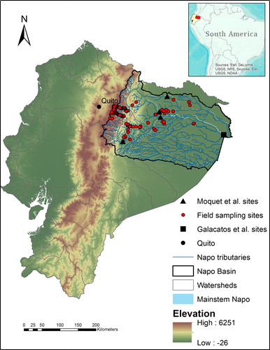
Figure 1. Map of Napo River Basin with elevation and field sampling site locations (2012–2014) provided and inset map showing location of Ecuador (yellow) and Napo River Basin (red). Locations of sampling areas from independent datasets from Galacatos et al. (2004) and Moquet et al. (2011) also provided.

Methods

Study area

The Napo River, a main tributary of the Amazon, comprises an altitudinal gradient of more than 5000 m, from which thousands of streams and rivers run through more than 31 phytogeographical formations (Ministerio del Ambiente del Ecuador 2012. The majority of the rivers in the Napo Basin (such as Napo, Coca, Tiputini, Yasuní, Curaray) are known as ‘aguas blancas’ (whitewaters) (Barriga 1994). The whitewater systems are originated in the Andean snowmelts and high altitude páramo grasslands at elevations over 4000 m, and have a muddy color caused by drainage which carries heavy sediment loads from eroding uplands (Galacatos et al. 2004). Another major type of rivers in the lower Napo Basin are the ‘aguas negras’ (blackwater) rivers, which originate in lowland swamps and flooded forests, and have a dark color associated with humic acids released through the decomposition of litter (Galacatos et al. 2004).

The Napo River is home to approximately 45,000 Kichwa speaking inhabitants and several thousands of other indigenous groups like the Waorani, Cofanes, Secoyas, between others (Torres-Carvajal et al. 2015). The Napo River Basin is estimated to harbor over 500 freshwater fish species, many of which are endemic to the region (Barriga 1994; Galacatos et al. 2004). It is also one of the most biologically diverse ecoregions in the world for amphibians, birds and mammals (Olson 1998; Bass et al. 2010; Jenkins et al. 2013a, 2013b; Lessmann et al. 2016). This high diversity in the Napo Basin can be attributed to several factors including its high altitudinal gradient (100–5500 m) which provides a great variety of physical and climatic conditions (Mena et al. 2006) and incredible heterogeneity of habitats. These practices can affect species community viability and biodiversity, as well as environmental services for human populations (Encalada 2010).

Field sampling

We sampled physicochemical parameters in situ at 165 field sites throughout the Napo River Basin from 2012 to 2014 to assess ecological integrity and species distribution modeling (see Lessmann et al. 2016, Figure 1). To assess the biological composition, we sampled aquatic macroinvertebrates classified into families and rated by their physiological tolerance according to the Andean Biotic Index (ABI; Acosta et al. 2009). We then used the ABI to determine an Average Score Per Taxa (ASPT), which indicates the biological integrity of the stream. The ASPT is the mean measure for the ABI scores of all families found in the river.

We evaluated habitat quality using the Riparian Quality Index (QBR) and Fluvial Habitat Index (IHF). The QBR index incorporates four measurements: degree of riverbank vegetation coverage, structure of vegetation cover, quality of the cover and degree naturalness of the riverbank. IHF incorporates variables, such as stream velocity, depth, frequency of riffles, substrate diversity, substrate composition and primary producer composition (Pardo et al. 2002). Both indexes were evaluated under the CERA protocol (Acosta et al. 2009), which is pre-established to fit specific characteristics of the eastern Ecuadorian high and mid lands.

All the parameters (ASPT, QBR, IHF) were normalized to fit a scale of 0-1, and averaged within each component. Then, we averaged the values obtained for the three components to generate an Ecological Integrity Index (EII), where an EII value of 0 indicated the poorest ecological integrity (i.e. highly impacted sites), while a value of 1 indicated the highest integrity.

We took effort to standardize sampling across years and did not use sites that were considered highly impacted (n = 4; EII <0.1) in the ecological integrity assessment (Lessmann et al. 2016). For model predictions, we used the mean of data points for each parameter across the 3 years. We measured all physicochemical parameters in situ from surface water samples. We measured conductivity (μS/cm), pH, and temperature (°C) using a YSI Model 63. Because conductivity is highly correlated with water temperatures, we reported all values standardized at 25 °C (i.e. specific conductance). Dissolved oxygen (mg/L) was measured using a YSI Model 550 A. We took measurements in triplicates and the average value of each site was employed.

Catchment delineation

Following methods in Auerbach et al. (2016) to delineate catchments, we generated values of flow accumulation for each cell in the elevation raster with the r.watershed tool (via GRASS functionality in QGIS 2.4). We then established a flow accumulation threshold for segment basin delineation according to: $${sb}_{\mathit{\text{threshold}}}=c\mathrm{*}\mathit{\text{mean}}(fac>0)$$

In this expression, the c coefficient on the mean of the non-zero values of flow accumulation serves to control the coarseness of the segment basin ‘mesh’ (in addition to the implicit scaling due to study extent). For the Napo, we set c = 3 with sb_threshold = 9797 (≈79 km²).

Model development

Spatial autocorrelation is based on the assumption that objects which are close to one another are more alike than those farther away (quantified here as spatial autocorrelation, Miller 2004). Geostatistical models use properties of spatial correlation to predict parameters based on distance from observed data in a process called interpolation (Clark 1979). Kriging is one of the most common forms of spatial interpolation and works by using the distance between observations and target points to make predictions while also accounting for the spatial design of the observations (Fortin et al. 2002; Gardner et al. 2003; Cressie and Wikle 2011). The problem with kriging along stream networks is that predictions are commonly based on Euclidean distance or the ‘shortest path’ between locations. However, Euclidean distance may not be an appropriate metric to use when examining locations linked in a network system such as a stream or a river because movement of organisms and material in a stream and river systems is restricted to the network (Little et al. 1997).

Topographical kriging or top-kriging is a method for estimating streamflow related variables in unsampled catchments (sub-watersheds). The model deals with the issue of Euclidean distance and connectivity by assuming stream flow to be generated by a spatially continuous process which exists at any point in the landscape, and stream flow measurements represent an aggregate (integral) of point runoff over a catchment (Laaha et al. 2013). Top-kriging estimates takes the area and the nested nature of catchments into account rather than estimating point based processes along the stream network (Skøien et al. 2006). Hydrologic distance can be either symmetric or asymmetric and is simply the distance between two locations when movement is restricted to the stream network.

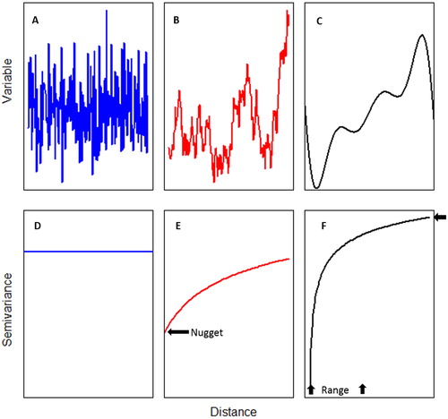
To make predictions, kriging uses a known covariance structure commonly represented by a variogram or more commonly a semivariogram which is simply one half of the variogram (Figure 2). A semivariogram is then used to explore the relationship where pairs that are close in distance should have smaller measurement differences than those separated by greater distances (Figure 2). The part of the semivariogram where the model first levels out or flattens is called the ‘range’ (Figure 2; Panel F). Sample locations separated by distances closer than the range are considered to be spatially autocorrelated, whereas locations farther apart than the range are not.

Figure 2. One-dimensional examples in which the data function (on top) give rise to the variogram (on the bottom). Panel A (blue line) exhibits no spatial autocorrelation, and hence results in a flat variogram (Panel D); Panel B (red line) exhibits spatial autocorrelation and random variation producing a variogram (Panel E) that rises slightly from a positive y intercept; Panel C (black line) is spatially autocorrelated and has no random variation so the variogram (Panel F) has a zero y-intercept. The value that the semivariogram model attains at the ‘range’ (the value on the y-axis) is called the ‘sill’. The ‘nugget’ is the location of the semivariogram origin on the y-axis.

We defined a stream segment as the portion of a stream located between two confluences. At each confluence or survey site in the network, we calculated the total upstream watershed area by summing the watershed area for incoming stream segments. The proportional influence for each incoming segment was calculated by dividing its watershed area by the total upstream watershed area at the confluence or survey site. The path between flow connected sites was estimated calculated the influence of one site on another, which was equal to the product of the segment proportional influences found in the path. The total distance traveled in the downstream direction is calculated which provides sufficient information to calculate hydrologic distance. If two sites were not connected by flow the spatial weight was equal to zero and a site’s influence on itself was equal to one (Peterson et al. 2006).

Interpretation of different types of simulated semivariograms is provided in Figure 2, where Panels A and D represent a pure nugget effect (i.e. no spatial autocorrelation), Panels B and E represent a combination of random variation and spatial autocorrelation and Panels C and F represent high spatial autocorrelations with no random variation. The value that the semivariogram model attains at the range (the value on the y-axis) is called the sill (Figure 2; Panel F). The nugget is the location of the semivariogram origin on the y-axis (Figure 2; Panel E). A nugget effect occurs when the nugget is greater than zero and can be attributed to measurement errors or spatial sources of variation at distances smaller than the sampling interval.

There are two main groups of forcings that control stream flow. The first group consists of variables that are continuous in space, such as rainfall, evapotranspiration and soil characteristics, which are related to local runoff generation. The second group is related to runoff aggregation and routing along the stream network. The main idea of top-kriging is to combine the two groups of forcings in a geostatistical framework that takes the river network topology into account. In top-kriging, the measurements are not point values but are defined over a non-zero catchment area (Little et al. 1997). We fit semivariogram models for each parameter by defining a least squares line that provides the best fit through the point pairs in the empirical semivariogram. We then determined the kriging weights, based on spatial autocorrelation from the semivariogram model, and assigned the weights to each measured values. We then calculated a prediction and variance for locations with unknown values based on the kriging weights.

To test the accuracy of our predictive models, we used leave-one-out cross-validation (LOOCV) (Hawkins et al. 2003). Similarly to jackknife tests, LOOCV works by running the model once for each value, using all other instances as a training set and using the selected value as a single-item test set. The process is repeated for each value in the data set. We then used a linear model to test our predicted values against the data removed for model testing, allowing us to describe the goodness of fit (GOF) of our models.

Model prediction validation

We also tested our model predictions for conductivity and pH through comparison to an independent dataset from Moquet et al. (2011). Their study included observed conductivity and pH ranges from five sites in four different sub-basins (Jatunyacu, Napo, Coca, Aquarico) in the Napo collected from 2000 to 2008 (see Figure 1; ‘Moquet et al. sites’). Because Moquet et al. (2011) provided data ranges for four sub-basins, we were able to statistically test our model predictions against their observed data for the two parameters to further evaluate our model. Among the most common and simple approaches to evaluate models is to regress predicted vs. observed values and compare the slope and intercept parameters against the 1:1 line (i.e. a perfect match between hypothetical observed and predicted values). If the lines are significantly different, the predicted values do not correspond well with observed values, indicating poor model predictions, while a not significant result indicates better correspondence between observed and predicted values. We also used an independent dataset collected by Galacatos et al. (2004) (see Figure 1 ‘Galacatos et al. sites’) in Yasuni National Park in the far eastern extreme of the Ecuadorian Napo Basin near the Peru-Ecuador border to test the precision of our estimates. Because all sites from that study were found within a single catchment, we could not conduct a statistical validation. However, the ranges provided by the study provide a useful non-statistical comparison for our predictions in one of the most distant catchments to our field sampling sites. All geostatistical analyses were conducted in Program R version 3.1.1 using package ‘rtop’. Physicochemical maps based on modeled predictions were constructed in ArcMap 10.2.

Results

Field sampling results (2012–2014)

Observed pH values ranged from 3 to 9 with eastern, lowland portions of the basin being generally more acidic, higher altitude sub-basins in the western part of the Napo were more basic, and intermediate elevations in the middle and southern portions of the watershed had more neutral pH. Conductivity values ranged from 5 to 257 (µS/cm), though there was no clear pattern with catchments ranging in conductivity values throughout the watershed but the predicted range was very similar to observed values (Figure 4). Dissolved oxygen at sampling sites ranged from 0.04 to 9.5 mg/L with catchments at higher altitudes in the western portion of the basin having higher levels of dissolved oxygen than in the eastern lowlands. Finally, temperatures ranged from 7 to 27 °C and were lowest in the western highlands, though some lowland areas exhibited fairly low stream temperatures, likely as a result of overhead shading and groundwater inputs.

Model results and validation

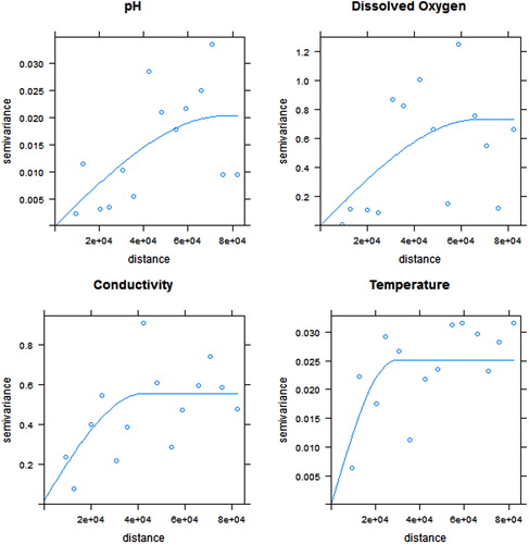
The semivariograms for each parameter showed a strong correlation between samples as a function of distance (Figure 3). The range, sill, and nuget for each parameter differed, indicating that the distances at which observations were spatially autocorrelated depended on the parameter (Figure 3). pH had the longest range, giving more confidence in predictions made at greater distances away from sample sites than for temperature predictions, which had the shortest range (Figure 3). Conductivity and dissolved oxygen had intermediate ranges (Figure 3).

Figure 3. Empirical semivariograms for environmental parameters depicting the variation between values at increasing distances away from sample sites with least squares line of best fit.

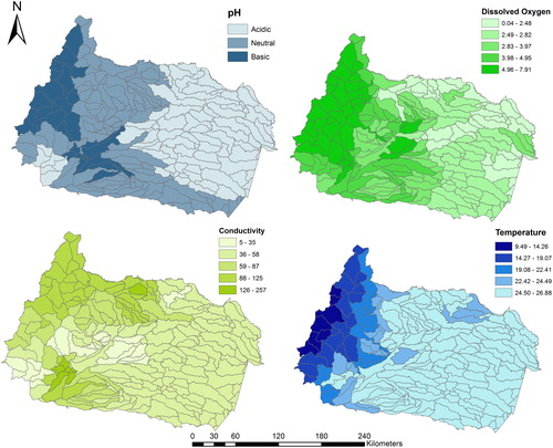
Basin-wide predicted pH values ranged from an average of 4 to 8, which was similar to the observed range (Figure 4). The predicted pattern was also similar to the observed pattern for pH with catchments in the eastern lowland portion of the basin being generally more acidic than the western highlands and neutral pH values in the central and southern portions of the basin. Conductivity predictions ranged from 5 to 266 (mS/cm) basin-wide, again with no clear elevational or longitudinal patterns (Figure 4). Predicted dissolved oxygen ranged from 0.04 to 7.10 (mg/L) with higher levels predicted in the western highlands (Figure 4). The smaller range of predicted values versus observed values for dissolved oxygen indicated that the model tended to over-simplify the observed values, though the predicted pattern was still similar to observed values. Basin-wide temperature predictions ranged 9.5–26.9 °C and showed a similar pattern to observed values (Figure 4).

Figure 4. Predicted values from top-kriging for pH, dissolved oxygen (mg/L), conductivity (mS/cm), and temperature (°C) within catchments. Sample site locations shown on each map as points.

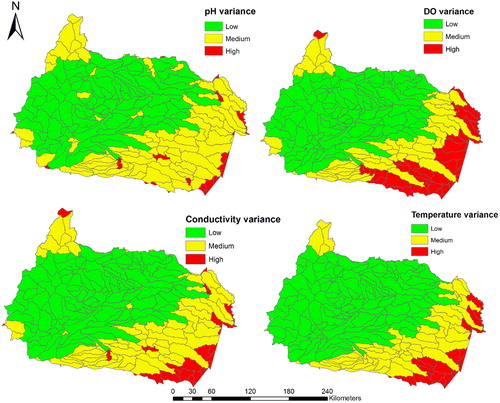
The strength of the spatial autocorrelation breaks down beyond a certain distance for each parameter as shown in Figure 3. In Figure 5, we provide scaled values of uncertainty based on variance levels for each parameter in every catchment within the Napo River Basin with red representing lower confidence in predictions and green representing higher confidence. As expected, variance (i.e. uncertainty) increased with greater distance from sampling sites for each parameter (Figure 5).

Figure 5. Variance ranges for each metric shown as low, medium, high to indicate relative confidence in predictions as distance from observed data locations increases. Red represents higher uncertainty and therefore lower confidence in predicted values.

LOOCV model validations showed a strong GOF for all parameters, as indicated by the coefficient of determination (R²). The GOF between observed and predicted stream temperature was highest (R² = 0.88), followed by pH (R² = 0.76). Conductivity and DO had slightly lower, though still high GOF, with R² values of 0.69 and 0.66, respectively.

When we tested our predicted conductivity ranges against the observed ranges from Moquet et al. (2011) (Table 1), the difference was not significant (Figure 6; P = 0.77; α = 0.05) indicating good fit between observed and predicted values. We repeated the procedure for observed versus predicted pH ranges, and again the difference was not significant (Figure 6; P = 0.9; α = 0.05).

Figure 6. Regression model line for predicted vs. observed pH values (Panel A) and conductivity (Panel B) compared to the 1:1 line (i.e. a perfect match between hypothetical observed and predicted values) (Piñeiro et al. 2008). If the lines are significantly different, the predicted values do not correspond well with observed values, indicating poor model predictions, while a not significant result indicates better correspondence between observed and predicted values. The difference between slopes for pH (P = 0.97) and conductivity (P = 0.77) and the 1:1 line were not significant indicating good fit between observed and predicted values for both parameters.

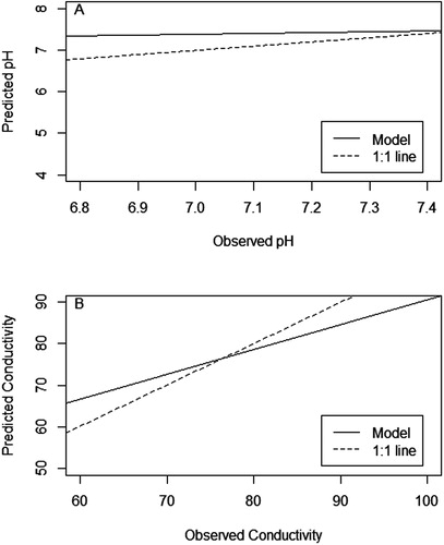
Table 1. Comparison of predicted within-catchment parameter ranges and observed parameter ranges in the same catchments from two independent datasets.

	Observed		Predicted
	Moquet et al. (2011)	Galacatos et al. (2004)	Alexiades et al. (2017)
pH	6–8.3	5.9–6.1	5.3–5.7
Conductivity (µS/cm)	62–66	58–67	45–64
Temperature (°C)	NA	26.2–26.7	25–26.7
Dissolved Oxygen (mg/L)	NA	0.9–1.1	0.04–2.48

For all four parameters, our predicted ranges overlapped, contained, or fell within the observed parameter ranges from Galacatos et al. (2004) (Table 1). While not a statistical test, the high degree of correspondence between observed and predicted values in a catchment where we had lower confidence in our predictions attests to the accuracy of our predictions.

Discussion

Physicochemical parameters, such as pH and stream temperature are primary determinant of freshwater ecosystem function and species community diversity, therefore understanding these factors is important for natural resource management and conservation in tropical basins. Our results provide the first comprehensive basin-wide estimates of stream physicochemical parameters for the Napo River Basin, one of the most biodiverse areas in the world for freshwater species. The estimates and methods in this study provide a tool to managers for present and future conservation efforts as human development in the Napo increases by establishing baseline estimates in areas with minimal disturbance. Furthermore, uncertainty analyses such as those in this study help to identify information gaps and direct efforts for future study and data collection. Models of stream physicochemistry fit better when predictors were catchment wide rather than more localized (Scott et al. 2002). By using top-kriging we provided a more appropriate method for making predictions along stream networks and in catchment than ordinary or universal kriging which require point-based estimates and utilize Euclidean distance.

Geostatistical spatial models such as top-kriging also provide estimates of uncertainty, which can be used to identify catchments where more monitoring sites are needed to optimize the stream water quality monitoring network. Given the statistical and spatial distribution of the observed data, it was not surprising that the models were able to predict physicochemical values more accurately in the western highlands, where available data were more abundant and widely distributed, than the eastern lowlands of the Napo. Future water quality monitoring efforts in the Napo should focus on the south eastern portion of the basin. Despite greater uncertainty in parameter estimates in the eastern lowlands of the Napo Basin, when our predicted parameter ranges were compared to independent datasets from the Napo Basin, they showed a high degree of correspondence.

The model developed in this study was intended to provide a reference baseline for four physicochemical parameters (pH, conductivity, temperature and dissolved oxygen) throughout the Napo River basin. Although the geostatistical model based on a limited set of factors fit the data well, there are potentially influential factors that were not adequately represented. For instance, observed differences in parameters may result from local factors, such as point sources of organic inputs or percent overhead cover, which were not incorporated at our scale of analysis. Local elevated pH or conductivity values could result from non-point sources of pollution, information which our lumped catchments were too general to capture. Additional information on the underlying geology, riparian and instream vegetation, and other biotic and abiotic factors would also improve predictions. We view these general predictions as vital to establishing baseline or natural conditions in the absence of anthropogenic disturbance (Peterson and Urquhart 2006). While it is doubtful that any of the observed or predicted catchments have not been altered in some way by human activities, we minimized these effects in our predictions by discarding highly impacted sites.

The results of our study indicate that spatial correlation exists in stream chemistry data at a relatively coarse scale and that geostatistical models improve the accuracy of predictions in a large, physically and ecologically diverse tropical watershed. The ranges and patterns of spatial correlation differ between chemical response variables, which are influenced by ecological processes acting at different spatial and temporal filter scales. The methods used in this study could be applied to data-scarce basins in other countries and regions where logistics or budget constraints preclude direct water quality sampling.

Implications for tropical biodiversity and conservation

Water resource managers and environmental planners are challenged to make informed, environmentally sound decisions that balance human and ecosystem needs. This challenge is especially acute where data-scarcity coincides with population growth, burgeoning resource development, and high freshwater species biodiversity. The framework outlined here provides a systematic and quantitative depiction of stream physico-chemistry at policy-relevant spatial scales. The proposed technique is flexible and can incorporate additional or alternative data sets, such as higher resolution, region-specific land cover, or additional geochemical attributes.

Human alteration of environmental conditions can greatly change species assemblage structure, diversity, and ecosystem function. Physicochemical conditions in streams are primary determinants of species assemblage structure and diversity (Whiteside and McNatt 1972; Sakset et al. 2012), highlighting the need to understand baseline physicochemical conditions in the basin to inform future research, conservation, and management as development continues within the Napo River Basin and other tropical areas worldwide. Our physicochemical model predictions represent an initial step in better understanding the natural conditions in remote streams within the Napo River Basin and this method could be applied to other remote regions of the world where the availability of water quality information is limited.

Notes on contributors

Alexander V. Alexiades is an Associate Professor of Environmental Science and Biology at Heritage University. He conducted this research as a Fulbright Fellow in Ecuador.

Andrea C. Encalada is a Professor of Biology at Universidad San Francisco de Quito in Cumbaya, Ecuador.

Janeth Lessmann is a PhD Candidate in Ecology at Pontificia Universidad Católica de Chile in Santiago, Chile. She conducted work on this manuscript as a MSc Student at Universidad San Francisco de Quito in Cumbaya, Ecuador.

Juan M. Guayasamin is a Professor of Biology at Universidad San Francisco de Quito in Cumbaya, Ecuador.

Acknowledgements

We would especially like to thank our funding agencies that made this work possible including The Rufford Foundation, The Fulbright Program Ecuador. We would also like to thank all the students and technicians of the USFQ Lab of Aquatic Ecology for their help and support. Finally, we would like to thank Dan Auerbach and Brian Buchanan for sharing their watershed delineation methods.

Disclosure Statement

No potential conflict of interest was reported by the authors.

Additional information

Funding

This work was supported partially by Partnerships for Enhanced Engagement in Research Science [grant number P1-108], Dimensions of Biodiversity grant from the National Science Foundation [grant number DEB-1046408], and Collaboration grant USFQ (‘Recursos de agua dulce y biodiversidad en la Cuenca del Napo’ to ACE).

References

- Acosta R, Ríos B, Rieradevall M, Prat N. 2009. Propuesta de un protocolo de evaluación de la calidad ecológica de ríos andinos (CERA) y su aplicación a dos cuencas en Ecuador y Perú. Limnetica. 28:035–064.
- Alexiades, AV, Flecker AS, Kraft CE. 2017. Nonnative fish stocking alters stream ecosystem nutrient dynamics. Ecol Appl. 27:956–965.
- Auerbach DA, Buchanan BP, Alexiades AV, Anderson EP, Encalada AC, Larson EI, McManamay RA, Poe GL, Walter MT, Flecker AS. 2016. Towards catchment classification in data-scarce regions. Ecohydrology 9:1235–1247.
- Barriga R. 1994. Peces del Parque Nacional Yasuní. Politécnica 19 (2) Biología. 4:9–41.
- Bass MS, Finer M, Jenkins CN, Kreft H, Cisneros-Heredia DF, McCracken SF, Pitman NC, English PH, Swing K, Villa G, et al. 2010. Global conservation significance of Ecuador’s Yasuní National Park. PloS One. 5(1):e8767.
- Buytaert W, Bièvre BD. 2012. Water for cities: The impact of climate change and demographic growth in the tropical Andes. Water Resour Res. 48
- Clark I. 1979. Practical geostatistics. London: Applied Science Publishers.
- Costanza R, d'Arge R, de Groot R, Farber S, Grasso M, Hannon B, Limburg K, Naeem S, O'Neill RV, Paruelo J, et al. 1998. The value of the world’s ecosystem services and natural capital. Ecol Econ. 25(1):3–15.,
- Cressie NAC, Wikle CK. 2011. Statistics for spatio-temporal data. Hoboken, NJ: Wiley.
- Dudgeon D. 2000. Large-Scale Hydrological Changes in Tropical Asia: prospects for riverine biodiversity the construction of large dams will have an impact on the biodiversity of tropical Asian rivers and their associated wetlands. Bioscience. 50:793–806.
- Encalada A. 2010. Funciones ecosistémicas y diversidad de los ríos: Reflexiones sobre el concepto de caudal ecológico y su aplicación en el Ecuador. Polémika 5.
- Finer M, Jenkins CN. 2012. Proliferation of hydroelectric dams in the Andean Amazon and implications for Andes-Amazon connectivity. PLoS One. 7(4):e35126.
- Fortin M, Dale MR, Ver Hoef JM. 2002. Spatial analysis in ecology. Encyclopedia of environmetrics. Chichester: Wiley.
- Galacatos K, Barriga-Salazar R, Stewart DJ. 2004. Seasonal and habitat influences on fish communities within the lower Yasuni River basin of the Ecuadorian Amazon. Environ Biol Fishes. 71(1):33–51.
- Gardner B, Sullivan PJ, Jr AJL. 2003. Predicting stream temperatures: geostatistical model comparison using alternative distance metrics. Can J Fish Aquat Sci. 60(3):344–351.
- Hawkins DM, Basak SC, Mills D. 2003. Assessing model fit by cross-validation. J Chem Inf Comput Sci. 43(2):579–586.
- Ibarra H. 2010. Visión histórico política de la Constitución del 2008. CAAP, Centro Andino de Acción Popular.
- ICA (Intelligence Community Assessment). 2012. IC paper on Global Water Security.
- Jenkins CN, Guénard B, Diamond SE, Weiser MD, Dunn RR. 2013a. Conservation implications of divergent global patterns of ant and vertebrate diversity. Divers Distrib. 19(8):1084–1092.
- Jenkins CN, Pimm SL, Joppa LN. 2013b. Global patterns of terrestrial vertebrate diversity and conservation. Proc Natl Acad Sci. 110(28):E2602–E2610.
- Johnson L, Richards C, Host G, Arthur J. 1997. Landscape influences on water chemistry in Midwestern stream ecosystems. Freshwater Biol. 37(1):193–208.
- Laaha G, Skøien JO, Nobilis F, Blöschl G. 2013. Spatial prediction of stream temperatures using Top-kriging with an external drift. Environ Model Assess. 18(6):671–683.
- Lessmann J, Guayasamin JM, Casner KL, Flecker AS, Funk WC, Ghalambor CK, Gill BA, Jácome-Negrete I, Kondratieff BC, Poff LN, et al. 2016. Freshwater vertebrate and invertebrate diversity patterns in an Andean-Amazon basin: implications for conservation efforts. Neotrop Biodivers. 2(1):99–114.
- Little LS, Edwards D, Porter DE. 1997. Kriging in estuaries: as the crow flies, or as the fish swims?. J Exp Mar Biol Ecol. 213(1):1–11.
- Mena CF, Bilsborrow RE, McClain ME. 2006. Socioeconomic drivers of deforestation in the Northern Ecuadorian Amazon. Environ Manag. 37(6):802–815.
- Miller HJ. 2004. Tobler’s first law and spatial analysis. Ann Assoc Am Geogr. 94(2):284–289.
- Ministerio del Ambiente del Ecuador. 2012. Sistema de clasificación de los ecosistemas del Ecuador continental. Quito: Subsecretaría de Patrimonio Natural.
- Moquet J-S, Crave A, Viers J, Seyler P, Armijos E, Bourrel L, Chavarri E, Lagane C, Laraque A, Casimiro WSL, et al. 2011. Chemical weathering and atmospheric/soil CO2 uptake in the Andean and Foreland Amazon basins. Chem Geol .287:1–26.
- Olson DP. 1998. Freshwater biodiversity of Latin America and the Caribbean: a conservation assessment: report of a Workshop on the Conservation of Freshwater Biodiversity in Latin America and the Caribbean held in Santa Cruz, Bolivia, September 27-30, 1995. Biodiversity Support Program.
- Pardo I, Álvarez M, Casas J, Moreno JL, Vivas S, Bonada N, Alba-Tercedor J, Jáimez-Cuéllar P, Moyà G, Prat N, et al. 2002. El hábitat de los ríos mediterráneos. Diseño de un índice de diversidad de hábitat. Limnetica. 21115–133.
- Peterson EE, Merton AA, Theobald DM, Urquhart NS. 2006. Patterns of spatial autocorrelation in stream water chemistry. Environ Monit Assess. 121:569–594.
- Peterson EE, Urquhart NS. 2006. Predicting water quality impaired stream segments using landscape-scale data and a regional geostatistical model: a case study in Maryland. Environ Monit Assess. 121613–636.
- Piñeiro G, Perelman S, Guerschman JP, Paruelo JM. 2008. How to evaluate models: observed vs. predicted or predicted vs. observed?. Ecol Modell. 216(3-4):316–322.
- Poff N, Richter B, Arthington A, Bunn S, Naiman RJ, Kendy E, Acreman M, Apse C, Bledsoe B, Freeman M, et al. 2010. The ecological limits of hydrologic alteration (ELOHA): a new framework for developing regional environmental flow standards. Freshwater Biol. 55(1):147–170.
- Potes V. 2010. Análisis de la aplicación del Derecho Ambiental en la Amazonía Ecuatoriana y el rol de las Fiscalías Ambientales. CEDA.
- Prusha BA, Clements WH. 2004. Landscape attributes, dissolved organic C, and metal bioaccumulation in aquatic macroinvertebrates (Arkansas River Basin, Colorado). J N Am Benthol Soc. 23(2):327–339.
- Sakset A, Gallardo WG, Ikejima K. 2012. Physicochemical conditions and biodiversity in the freshwater fishing area of Pak Phanang River Basin, Thailand. Int J Sustain Dev World Ecol. 19(2):172–188.
- San Sebastián M, Karin Hurtig A. 2004. Oil exploitation in the Amazon basin of Ecuador: a public health emergency. Rev Panam Salud Pública. 15:205–211.
- Scott MC, Helfman GS, McTammany ME, Benfield EF, Bolstad PV. 2002. Multiscale influences on physical and chemical stream conditions across Blue Ridge landscapes. J Am Water Resour Assoc. 38(5):1379–1392.
- Skøien JO, Merz R, Blöschl G. 2006. Top-kriging-geostatistics on stream networks. Hydrol Earth Syst Sci. 10(2):277–287.
- Torres-Carvajal O, Salazar-Valenzuela D, Merino-Viteri A, Nicolalde DA. (n.d.). ReptiliaWebEcuador. Versión 2015. 0. Quito: Museo de Zoología QCAZ, Pontificia Universidad Católica del Ecuador; 2015.
- Townsend, CR. 2003. Individual, population, community, and ecosystem consequences of a fish invader in New Zealand streams. Conser Biol. 17:38–47
- Whiteside BG, McNatt RM. 1972. Fish species diversity in relation to stream order and physicochemical conditions in the Plum Creek drainage basin. Am Midland Nat. 88(1):90–101.
- World Wildlife Fund. 2014. Napo Moist Forests.