Effects of groundwater fluctuations on the distribution and population structure of two cyprinid fishes in a desert spring complex

Abstract

Relationships between groundwater levels, surface water levels, and the distribution and habitat use of two cyprinid fishes, Least Chub (Iotichthys phlegethontis) and Utah Chub (Gila atraria), were examined at a spring complex in the Snake Valley of the Great Basin, USA to test the hypothesis that the distribution and structure of fish populations in the spring complex is regulated by the influence of shallow groundwater levels on the depth and distribution of surface water and the availability of suitable spawning and juvenile habitat. Groundwater levels explained 97% of the temporal variation in surface water levels measured at 47 monitoring points and exhibited annual cycles linked to evapotranspiration rates. Least Chub and Utah Chub migrated from springs to ponds, which were used as spawning and juvenile habitat, when groundwater and surface water levels were high during the early spring, but became concentrated in deep springs as ponds receded during the late summer and early fall. Populations of both species became increasingly fragmented as groundwater and surface water levels declined. Specific differences in the relative abundances and body sizes of juvenile Least Chub inhabiting different seasonally isolated regions of the spring complex persisted over multiple years, suggesting that juvenile growth rates and survival were influenced by connectivity of core spring habitats to seasonally deep ponds. The nature of the relationship between groundwater and surface water levels indicated that long-term declines in shallow groundwater levels of ≥ 40 cm would eliminate most of the spawning and juvenile habitat in the spring complex.

Keywords:

• Gila atraria
• Great Basin
• groundwater
• habitat fragmentation
• Iotichthys phlegethontis
• Snake Valley
• springs

Introduction

The Great Basin covers more than 540,000 km² of western North America and encompasses a region of numerous north-south trending mountain ranges and valleys that form a series of contiguous endorheic drainages. This basin and range topography began forming approximately 17.5 million years ago, during the Early Miocene, and created a geological template favoring the formation of unique assemblages of aquatic organisms. Beginning about 3 million years ago, a trend toward increasing aridity associated with the uplift of the Sierra Nevada Mountains contributed to the loss and fragmentation of aquatic ecosystems in the Great Basin. The arid conditions and isolation of aquatic ecosystems caused high extinction rates among populations of fish and aquatic invertebrates and resulted in a modern fish fauna characterized by low species diversity and high endemism (Hubbs et al. 1974; Sada and Vinyard 2002; Smith et al. 2010).

Impacts to aquatic ecosystems of the Great Basin caused by human activities, including the dewatering of streams through agricultural diversions and the loss or reduction of spring habitats due to groundwater pumping, have resulted in recent contractions in the distribution and abundance of many of the endemic fishes. Most of the spring systems of the region are supplied with groundwater from shallow basin-fill aquifers connected to deep carbonate-rock aquifers. These aquifers are currently being depleted to varying degrees by groundwater removal. In extreme cases, pumping has reduced water table levels and spring discharge rates to the extent that losses of phreatophytic vegetation and extinctions of populations of fish and other aquatic organisms have occurred (Deacon et al. 2007; Patten et al. 2008; Gardner and Heilweil 2014).

Recent controversy over conflicting demands for groundwater in the Great Basin has focused on Snake Valley. Snake Valley covers an area of 3880 km² and extends more than 160 km along the border between the states of Nevada and Utah, USA in an area that was once inundated by a narrow southwestern extension of Lake Bonneville, a pluvial lake that covered more than 50,000 km² of the eastern Great Basin during the Late Pleistocene (Currey 1990; Oviatt 1997). Potential ecological and economic impacts of groundwater removal from Snake Valley became a critical issue following a proposal by the Southern Nevada Water Authority to pump groundwater from the deep carbonate-rock aquifer underlying the valley and from the connected aquifer underlying the nearest neighboring valley to the west (Spring Valley) to meet the demands of the Las Vegas, Nevada metropolitan area, a fast-growing and arid urban area inhabited by more than two million people and located > 450 km to the south of Snake Valley. To obtain baseline data to address these impacts, the Utah Geological Survey (UGS) began a long-term groundwater monitoring program in 2004 using a network of wells and piezometers distributed throughout the Utah portion of Snake Valley.

One of the focal areas in the UGS monitoring program in Snake Valley is the Leland Harris Spring Complex, a spring-fed marsh in the central portion of the valley that was selected for monitoring based on its ecological value (Hurlow 2014). I collected bathymetric data and data on temporal variation in surface water levels at the Leland Harris Spring Complex, in conjunction with groundwater monitoring data from a UGS well located to the west of the spring complex, to evaluate how variation in shallow groundwater levels (GWL) influences the habitats and populations of two cyprinid fishes, Least Chub (Iotichthys phlegethontis) and Utah Chub (Gila atraria). These data were used to test the hypothesis that fish distributions and population structure (i.e., relative abundance of juveniles) respond to changes in GWLs due to the influence of groundwater on the depth and distribution of surface water and the availability of suitable spawning and juvenile habitat. The study had four primary objectives: (1) documenting patterns of temporal variation in shallow GWLs and how this variation is related to climate variables, (2) quantifying the strength and nature of the relationship between surface water levels and shallow GWLs, (3) evaluating temporal changes in the distribution of Least Chub and Utah Chub (e.g., migration and seasonal use of spawning and juvenile habitat) in relation to temporal variation in the depths and distribution of surface water, and (4) documenting persistent differences in the relative abundances and body sizes of juvenile and adult Least Chub in different regions of the spring complex that become isolated from one another during periods of habitat contraction.

Materials and methods

Study area

The Leland Harris Spring Complex forms a marsh covering 0.42 km² (42 hectares) in the central portion of Snake Valley in Utah at 39°33′N and 113°53′W (Figure 1). It ranges from 1456 to 1458 m in elevation and is the northernmost of a series of three isolated spring complexes in Snake Valley that provide much of the remaining habitat for Least Chub, a species endemic to the area of the eastern Great Basin formerly occupied by Lake Bonneville (Bonneville Basin). Shallow groundwater flows into the Leland Harris Spring Complex from the west along a downward hydraulic gradient before encountering an impermeable layer, where an upward hydraulic gradient forms and causes groundwater to emerge from > 60 springs, most of which originate near the western edge of the marsh and flow to the east and northeast into low basins to form shallow ponds. The majority of these ponds are perennial but fluctuate greatly in depth and volume, but some are relatively stable and a few are ephemeral (Grover 2016).

Figure 1. Map of the Leland Harris Spring Complex showing bathymetry isolines, locations of UGS shallow groundwater monitoring well SG25D, surface water and fish visual monitoring sites, and additional monitoring sites where visual surveys of fish were conducted from April through October 2013.

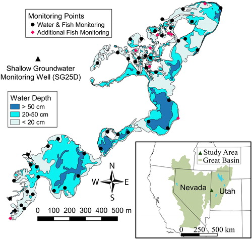
Least Chub and Utah Chub are the only fishes that inhabit the Leland Harris Spring Complex. Least Chub represent the only species in the genus Iotichthys, which has been a distinct lineage in the eastern North America shiner clade of the minnow family (Cyprinidae) for approximately four million years (Smith et al. 2002; Estabrook et al. 2007; Houston et al. 2010). They are small (28–65 mm total length as adults) omnivorous fish that forage opportunistically on insect larvae, crustaceans, and algae (Sigler and Sigler 1987). Least Chub were once common in springs, lake margins, and low-gradient streams throughout much of the Bonneville Basin in Utah, but declined in distribution and abundance due to impacts caused by habitat loss and degradation combined with introductions of non-native fishes. Only six viable populations of naturally occurring Least Chub remain, three of which are in Snake Valley (Sigler and Sigler 1987; United States Fish and Wildlife Service 2014). Least Chub are fractional spawners. At the Leland Harris Spring Complex they typically begin spawning in April and can continue spawning into the summer until as late as August (Crawford 1979). Utah Chub are cyprinids in the western North America chub clade that are found in the Bonneville Basin and the Upper Snake River drainage, which were connected on two occasions during the Pleistocene (Smith et al. 2002). They are often abundant in lakes, reservoirs, spring systems, and low-gradient streams. Juveniles feed primarily on zooplankton, whereas adults tend to have a more diverse diet consisting of aquatic insects, crustaceans, diatoms, and vascular plants (Rees 1935). The species exhibits a high degree of life-history variation and ecological plasticity. Age at maturity varies from 2 to 6 years and size at maturity can range from 65 to > 200 mm total length (TL), depending on the population, environmental conditions, and the influence natural selection resulting from predation by piscivorous fish (Johnson 2002, Williams et al. 2017). Utah Chub are not known to prey on Least Chub, and the two species are positively associated with one another at multiple spatial scales in the Leland Harris Spring Complex (Grover 2016).

Groundwater and climate data

Data on shallow GWLs at a UGS monitoring well (SG25D) located approximately 335 m to the west of the Leland Harris Spring Complex were obtained from the UGS website (http://apps.geology.utah.gov/groundwater/site.php?site_id=25, accessed on 25 February 2018). The monitoring well, which is 35.4 m deep and located at an elevation of 1461.6 m, is equipped with a pressure transducer data logger housed within a 5.1 cm diameter slotted and screened PVC pipe placed within a 10.2 cm wide steel casing. Hourly data on GWLs were obtained for dates between 1 August 2012 and 31 August 2014 and were recorded as the difference in elevation between the top of the water column in the monitoring well and the ground level, to the nearest 0.1 cm. The hourly measurements were used to calculate daily averages of GWLs on days when surface water monitoring took place. In addition, monthly averages from February 2009 (when the data logger was installed) to December 2017 were calculated and used to investigate long-term relationships between GWLs, evapotranspiration, and precipitation. The data logger in the monitoring well was nonfunctional during 10 months between June 2016 and July 2017, but average GWLs at SG25D during those months were estimated using predicted values from the regression equation describing relationships of water levels at SG25D to those at an additional monitoring well (SG25C) located at the western edge of the spring complex (GWL_SG25D = 1.32·GWL_SG25C – 205.41, n = 95, r² = 0.959).

Precipitation data and reference potential evapotranspiration (ET_o) rates were obtained from the Utah Climate Center database (https://climate.usurf.usu.edu) for a weather station located 7.5 km to the north of the spring complex in Partoun, Utah (ID: USC00426708). The ET_o rates provided by the Utah Climate Center were based on temperature data from the weather station and were estimated using the Hargreaves method (Hargreaves and Samani 1985). The weather station was at the same elevation as the spring complex (1457 m) and experienced amounts and patterns of precipitation similar to those recorded during 2012–2014 at a rain gauge located in the spring complex (Grover 2016). These data were used to examine relationships between monthly averages of GWLs, monthly precipitation totals, and estimated ET_o rates from February 2009 through December 2017 as a means of evaluating long-term relationships between GWLs, evapotranspiration and precipitation.

The relationships between GWLs and climate variables were explored using stepwise linear regression analyses in which precipitation totals during intervals including or preceding the groundwater measurements (precipitation totals to the nearest mm during the same month, previous month, previous 2 months, or previous 3 months), and average evapotranspiration (ET_o) rates during these same intervals were used as independent variables. The mean GWL at monitoring well SG25D during each month from February 2009 through December 2017 was the dependent variable. The best fit equation was the one in which the selected time frames of the ET_o and precipitation measurements explained the most month-to-month variation in GWLs.

Surface water monitoring

During the period beginning 5 October 2012 and ending on 17 August 2014, I measured surface water depths on 15 occasions at 47 monitoring points, 23 of which were located at the heads of springs or in outflow channels and 24 of which were located in ponds within a few meters of the shoreline. Monitoring points were established at all large springs and most ponds at locations that were easily accessible from the shoreline, and were somewhat clustered in the central portion of the northeast region of the spring complex, where the density of springs and small ponds was highest. The spatial arrangement of the monitoring points facilitated documentation of site-specific changes in water levels over time throughout the spring complex. Each monitoring point was marked with a hollow 2 cm diameter aluminum pole measuring between 1.5 and 2.5 m in length and embedded securely in the substrate for the duration of the study. Water depths at monitoring points were measured using a 2.8 cm diameter ×170 cm long polyvinyl chloride (PVC) probe marked at 1 cm intervals and labeled at 5 cm intervals. The probe was always placed next to the north side of the pole that marked the monitoring point to ensure that measurements were consistently taken from the same location. Water depth was measured as the distance from the top of the uppermost layer of benthic sediments to the water’s surface. To correct for the influence of localized temporal changes in sediment thickness resulting from sediment transport, I also used a stainless steel meter stick to measure the distance (to the nearest 0.1 cm) from the water’s surface to the top of the pole that marked the location of the monitoring point and calculated surface water levels (SWL) at each point for each sampling date by subtracting the measured distance from the top of the pole to the water’s surface on the sampling date from the average distance from the top of the pole to the benthic sediments for all sampling dates. This provided a measure of the water level that was scaled to reflect the water depth as measured from the average level of the upper surface of the benthic sediments at the point. The SWL values were used in all analyses involving measurements of surface water levels at the 47 surface water monitoring points.

Water temperatures were measured opportunistically at ice-free bodies of water during three periods defined on the basis of temporal trends in fish habitat use: (1) the November-February overwintering period, (2) the April-June spawning period, and (3) the August-October post-spawning period. Measurements of pH and specific conductivity were also obtained periodically using an Extech® II pH/Conductivity meter. All measurements were taken approximately 5 cm below the surface of the water at springheads (upwellings), spring channels, and ponds. Large ponds were covered in thick ice during winter months, which limited winter sampling of ponds to open-water areas relatively close to inlets from spring channels.

Relationships between GWLs and surface water levels were explored using ordinary least-squares regression. Three regression analyses of GWLs on SWL measurements during the 15 monitoring periods were performed: one examining the relationship between the GWL and the average of the SWL levels measurements at all 47 surface water monitoring sites, one examining the groundwater-SWL relationship at the 23 monitoring sites located in springheads and channels, and another examining the relationship at the 24 sites located in ponds. Values of GWLs used in these analyses were the daily averages from the dates when the surface water measurements were obtained. The regression coefficients from the two analyses that considered ponds and spring separately were compared in a test of slope heterogeneity to evaluate whether ponds and springs differed in the degree to which their water levels changed in response to changing GWLs.

As a means of extrapolating surface water monitoring data from the monitoring points to larger scale variation in the distribution and depth of surface water, water depths were measured and recorded (to the nearest 0.5 cm) at 3852 points located throughout the Leland Harris Spring Complex during a bathymetric survey that began on 16 April 2013 and ended on 2 May 2013; described in detail in Grover (2016). The bathymetric survey was scheduled to coincide with the seasonal peak in surface water levels at the spring complex. A survey grade GPS unit (Ashtech MobileMapper® 100) was used to obtain the UTM coordinates (NAD 83, Zone 12 to the nearest 0.5 m) at each bathymetry point and to map the perimeter of each body of water in which bathymetric measurements were obtained. The bathymetric data were used to create isoline maps of the spring complex, estimate average water depths in different areas, and to estimate the combined area and volume of spring-fed bodies of water during each period when surface water monitoring took place.

Relationships between GWLs, the inundated surface area of the spring complex, and the volume of water in the spring complex on dates when surface water monitoring occurred were also examined. Surface water measurements at the 47 monitoring points were extrapolated to estimate water depths at points where bathymetry measurements had previously been obtained in the same bodies of water. The mean of the estimated water depths was multiplied by the surface area of all bodies of water in the spring complex, which was estimated from GPS data and GIS mapping of polygons encompassing the bathymetry points that were inundated at the time of the survey, to estimate the volume of surface water in the spring complex. Periodically inundated playas along the eastern edge and extending into the central portion of the spring complex were excluded from these estimates (and from surveys) because they were not supplied by spring water, tended to be highly saline and shallow when water was present, and were never inhabited by fish. The relationship between GWLs and the surface area of all spring-fed bodies of water was examined using a linear model and ordinary least squares regression. Nonlinear regression, using an exponential model, was used to explore how the volume of surface water in the spring complex changed with changing GWLs during 2012–2014.

Monitoring of fish distributions

Visual surveys of fish distributions were conducted concurrently with each of the surface water monitoring surveys. The visual surveys took place at 50 locations, most of which were centered at or near surface water monitoring points to ensure that all ponds and large springs in the spring complex were surveyed for fish during each monitoring period (Figure 3). Some of the visual survey areas encompassed multiple small springs that had seasonal surface connections. The visual survey protocol involved scanning the survey area from the shoreline and then wading slowly through the water within a 10 m radius of the monitoring point and searching for fish, noting the locations of any fish observed and identifying which species and age groups were present. Depending on the amount of vegetative cover, adults of both species could usually be approached and observed from a distance of 1–3 m before they fled. Larvae and small young-of-the-year juveniles (YOY) permitted closer observation. Water depths at visual survey areas were estimated from measurements obtained during the bathymetric survey adjusted for the current SWL at associated surface water monitoring points. Information from visual surveys, along with water depths at survey sites, was used to evaluate how the distributions of juveniles and adults of both species changed over time and how those changes were related to average water depths at survey sites. Because Least Chub reach sexual maturity within one year, all juvenile Least Chub that were observed were YOY (age 0). Age 1+ juvenile Utah Chub were often intermixed with YOY Utah Chub during late summer and fall, and it was assumed that shoals of small juveniles contained YOY during that time. For consistency all immature individuals (including larvae) were categorized as juveniles.

Visual survey areas were nonoverlapping, and each was delineated to include a minimum of 10 bathymetry points. Visual survey data were collected from October 2012 to August 2014. However, thick ice precluded observations of fish in several of the ponds in the spring complex during November 2012 through February 2013, and only three surveys were conducted during 2014. Consequently, only visual survey data collected on a monthly basis during April-October 2013, a period that spanned the migration of Least Chub and Utah Chub to and from spawning and juvenile habitats during a single year, were analyzed in this study.

Differences between water depths at sites in which individuals belonging to a specific age category (juvenile or adult) and species (Least Chub or Utah Chub) were observed during visual surveys and water depths at sites in which individuals of that species and age-class were not detected were assessed using Mann-Whitney U-tests. Separate tests were performed on monthly survey data from April through October 2013 for adult Least Chub and adult Utah Chub. Juveniles were not detected until May 2013, so only 6 months of visual survey data (May-October 2013) on juveniles were analyzed. The purpose of the multiple Mann-Whitney U-tests was to provide an objective method of distinguishing periods when juveniles and adults of each species were using deep-water habitats, not to test the hypothesis that habitats with relatively high average water depths were used more frequently than shallower habitats.

Population monitoring

I conducted population monitoring surveys to collect demographic data on Least Chub and Utah Chub during mid-August to late September of 2012–2014, when groundwater and surface water levels were seasonally low. The population monitoring surveys involved passive sampling using unbaited collapsible minnow traps set for 2–4 hours in water ≥ 7 cm deep. Each of the minnow traps measured 46 × 25 × 25 cm, had 6 cm diameter funnel openings at each end (large enough to accommodate the largest adults), and was made of polyethylene mesh (3 mm mesh size). Traps were usually placed on benthic sediments at locations where fish were observed prior to the set. At large springs, traps were set in approximately equal numbers in the springhead and downstream channel. In ponds dominated by shallow (< 25 cm deep) water, traps were set in areas deep enough to accommodate them regardless of whether fish were observed there. Captured fish were identified, counted, measured (total length to the nearest 1 mm, TL), and released on site immediately after measurements were obtained. Occasionally, when large numbers of fish were captured in a body of water, subsamples of ≥ 100 Least Chub and ≥ 50 Utah Chub were measured and the remaining individuals were identified, counted, and released without being measured. Data from these surveys were used to evaluate whether juveniles and adults differed in their distributions and habitat associations at a time when the majority of individuals had become concentrated in core habitats.

Length measurements of Least Chub obtained during the 2012–2014 population monitoring surveys were used to evaluate whether subpopulations that became seasonally isolated in different regions of the spring complex exhibited differences in juvenile TL measurements (reflecting differences in growth rates or other factors), differences in the proportion of juveniles in samples, and adult size differences. These data were relevant to the question of whether regional differences in habitat parameters within the spring complex can have a consistent influence on population structure and average juvenile and adult body size among groups of Least Chub that become isolated in specific regions due to habitat fragmentation. Adult Least Chub were distinguishable from juveniles by a combination of their size and reproductive traits (orange breeding coloration in males and more robust proportions associated with enlarged ovaries in females).

Seven seasonally isolated regions were identified based on habitat monitoring and visual surveys of fish. Between-region differences in TL measurements obtained from Least Chub were evaluated using separate ANOVAs for measurements of juveniles and adults from each year. Samples of juvenile Least Chub from one of these regions (Barbell Springs) were too small (0–6 individuals) to be included in the analyses of juvenile size differences. Differences in TL measurements between samples of Utah Chub captured from different regions of the spring complex during 2012–2014 were also examined, but the difficulty in distinguishing between year classes of juveniles and between large juveniles and small adults precluded analyses of age-specific size differences.

During the 2013 and 2014 population monitoring surveys, I recorded the water depths at all trap locations to evaluate whether traps that captured Least Chub or Utah Chub of a particular age category (juvenile or adult) tended to be located in microhabitats with deeper water than traps that failed to capture individuals of that age category. Juvenile Utah Chub require more than 1 year to reach sexual maturity, and age 1+ juveniles were often difficult to distinguish from adults on the basis of size and external features. Nonetheless, YOY and large adults were easily categorized, and the size range of all Utah Chub captured in a trap was a reliable indicator of whether juveniles and/or adults were present. Water depths of traps in which individuals belonging to a specific age category and species were captured were compared to water depths of traps that failed to capture individuals of that species and age category using separate Mann-Whitney U-tests for juveniles and adults of each species during each year.

Results

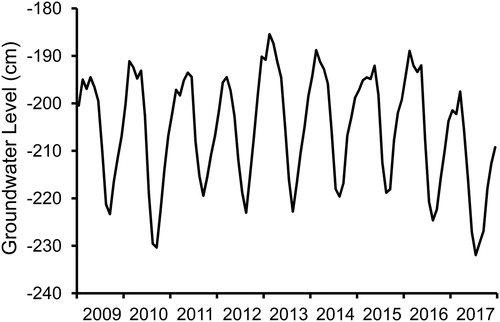
Shallow GWLs fluctuated seasonally at the Leland Harris Spring Complex during 2009–2017, peaking each year in winter and early spring and declining in mid to late summer (Figure 2). The mean GWL, in terms of the difference in elevation between the top of the water column in monitoring well SG25D and the well’s elevation at ground level, was −205.6 cm (SD = 11.7 cm, n = 107). Monthly averages peaked at −185.4 cm in February of 2013 and reached a low of −232.0 cm during July of 2017. The cyclic annual fluctuations in GWLs were much more prominent than between-year differences, and were linked to the mean ET_o during the preceding three months (r² = 0.741), with a very small but significant amount of additional variation accounted for by the precipitation total during the same month the groundwater measurements were obtained (GWL = −4.75· ET_o + 0.71·Precip – 189.48, R² = 0.755, F_2,104 = 160.32, P < 0.001). Annual precipitation totals were higher during 2009–2011 (22.8–28.5 cm) than during 2012–2017 (14.4–18.3 cm), whereas annual means of GWLs varied by only 6 cm until a drop from −204.0 to −214.9 cm occurred from 2016 to 2017. If precipitation trends had any influence on year-to-year variation in GWLs, the response was delayed multiple years.

Figure 2. Groundwater levels, in terms of monthly averages of water depths with respect to ground level, at shallow groundwater monitoring well SG25D at the Leland Harris Spring Complex from 2009 through 2017.

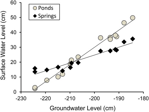
Mean values of the SWL measurements taken during 2012–2014 were tightly linked to GWLs (SWL = 0.86·GWL + 199.10, r² = 0.972, n = 15, P < 0.001). Surface water levels in ponds fluctuated to a greater degree with changing GWLs than surface water levels in springs (Figure 3), increasing approximately 1.2 cm, on average, for every 1 cm increase in GWL (SWL = 1.17·GWL + 264.56, r² = 0.989, P < 0.001), compared to an increase of less than 0.6 cm for springs (SWL = 0.56·GWL + 137.29, r² = 0.930, P < 0.001). A test for heterogeneity of slopes indicated that this difference was significant (F_{1, 26} = 104.2, P < 0.001). Differences between the highest and lowest measurements of SWL at individual monitoring points varied considerably depending on the location of the monitoring point, ranging from 2.0 to 36.1 cm at monitoring points in springs and from 6.4 to 73.5 cm at monitoring points in ponds.

Figure 3. Mean surface water levels measured at monitoring points in springs (n = 23) and ponds (n = 24) compared to shallow groundwater levels recorded on the same dates during 15 monitoring periods from October 2012 to August 2014.

The steepest decline in surface water levels occurred between February and August of 2013. GWLs recorded on monitoring dates declined 39.9 cm during that period. Corresponding declines in surface water levels at monitoring points at springs averaged 22.1 cm, compared to an average decline of 47.5 cm at monitoring sites in ponds. The relatively large reductions of surface water levels in ponds were likely attributable to the prevailing drainage pattern of the spring complex, in which water emerging and flowing from spring orifices accumulates in lower elevation pond basins, and to higher rates of evapotranspiration in ponds stemming from their larger surface area and the presence of emergent vegetation in shallow shoreline areas.

Specific conductivity measurements obtained from ponds averaged 1274.4 µs/cm (95% CI 978.3–1570.4 µs/cm, n = 47), compared to 612.1 µs/cm (95% CI 579.0–645.2 µs/cm, n = 76) at springheads and 625 µs/cm (95% CI 567.3–683.2 µs/cm, n = 37) in channels, indicating that solute concentrations tended to be relatively high in ponds. A similar between-habitat difference in pH levels was apparent, with pH measurements obtained from ponds averaging 8.68 (95% CI 8.46–8.90, n = 46), compared to 8.15 (95% CI 8.06–8.26, n = 76) in springheads and 8.16 (95% CI 8.03–8.27, n = 37) in channels.

The surface water depths, inundated surface area, and volume of water in the Leland Harris Spring Complex varied with changing GWLs during 2012–2014. Mean surface water depths peaked at 33–36 cm during January-February 2013 and declined to a low of around 18 cm during July-September 2013 (Table 1). The inundated surface area of the spring complex ranged from approximately nine to 34 hectares and most of this variation was explained by variation in GWLs (Area = 67.63·GWL + 161.89, r² = 0.947, P < 0.001). The estimated combined volume of all spring-fed bodies of water changed exponentially with changing GWLs (Vol. = 161,570e^3.85·GWL – 10.63, r² = 0.967, P < 0.001). The 0.4 m decline in GWLs that occurred from February to August of 2013 was accompanied by a 73% decline in the inundated area of the spring complex and an 81% decline in the volume of surface water. In addition, surface water depths declined by an average of 51% from February to July of 2013 despite the fact that only 38% of the area of the spring complex that was inundated during February was included in July depth measurements because the remaining area was dry. All springs and most ponds retained at least some surface water when GWLs were at their lowest, but discharge rates at some of the springs became too low to maintain connections with ponds, and reduced surface water levels in large ponds led to additional habitat loss and fragmentation.

Table 1. Groundwater level (GWL), mean surface water depth at inundated bathymetry points (SWD), estimated total inundated surface area, and estimated combined volume of all bodies of water in the Leland Harris Spring Complex during each period of surface water monitoring. The total number of bathymetry points was 3852, but only those inundated at the time of the survey were used in calculating surface water depths, area, and volume.

Date	GWL (cm)	SWD (cm)		Area (ha)	Volume (m^3)	Inundated Points
		Mean	SE
5 Oct 2012	−209.9	19.3	0.5	19.6	37,737	2719
14 Nov 2012	−197.5	25.5	0.4	33.1	84,225	3788
5 Jan 2013	−187.9	32.8	0.4	33.9	111,145	3851
18 Feb 2013	−184.4	36.1	0.5	33.9	122,218	3845
4 Apr 2013	−191.0	25.9	0.4	32.8	84,697	3769
2 May 2013	−191.5	26.3	0.4	33.6	88,506	3832
23 May 2013	−193.4	25.3	0.4	33.1	83,823	3793
20 Jun 2013	−206.7	21.0	0.5	20.9	43,911	2824
26 Jul 2013	−219.5	17.8	0.6	13.0	23,059	2200
21 Aug 2013	−224.3	18.2	0.7	9.1	16,460	1889
13 Sep 2013	−214.9	18.2	0.6	15.8	28,766	2424
21 Oct 2013	−209.4	20.3	0.5	22.7	46,160	2971
7 May 2014	−193.6	24.5	0.5	29.9	73,255	3580
8 Jul 2014	−213.1	18.6	0.6	14.5	26,970	2219
17 Aug 2014	−224.1	18.1	0.7	12.4	22,444	2033

Monthly visual surveys of fish at monitoring sites during April-October 2013 indicated that Least Chub and Utah Chub exhibited shifts in distribution and habitat use that were associated with fluctuations in water levels and with breeding activities. In many locations, adults of both species had moved from overwintering habitats in springs to spawning habitats in ponds by April (Table 2). At all but one of the core springs used as overwintering habitat, all Least Chub and Utah Chub departed for pond habitats simultaneously and no fish were detected at the spring during at least one visual survey in April or May. Sites occupied by Least Chub in April were significantly deeper than sites where Least Chub were not observed, whereas sites in which Utah Chub were observed in April were of similar depths to other monitoring sites (Figure 4). Larvae of both species were abundant in several ponds and a few springs by late May. Adults of both species were beginning to leave breeding ponds by that time. By late June, adult Least Chub and Utah Chub had largely migrated back to relatively deep springs, and the sites in which they were observed had significantly deeper water than sites in which they were not observed. Juveniles of both species were widely distributed in ponds during June, but were also present in several springs. Sites occupied by juvenile Utah Chub during June had significantly deeper water than sites in which juvenile Utah Chub were not detected, but this was not the case for juvenile Least Chub. Juvenile Utah Chub moved out of almost all shallow pond habitats before July. Both adult and juvenile Utah Chub remained in habitats with relatively deep water during the remainder of the visual survey period. By contrast, adult Least Chub occupied habitats with relatively deep water from June through October, but juvenile Least Chub remained in receding ponds until August.

Figure 4. Mean water depths (± 2 SE) at visual monitoring sites occupied by juvenile Least Chub, juvenile Utah Chub, adult Least Chub, and adult Utah Chub during surveys conducted from April to October of 2013. In all cases with non-overlapping error bars, Mann-Whitney U-tests indicated that there was a significant tendency for occupied sites to be deeper than unoccupied sites (P < 0.05).

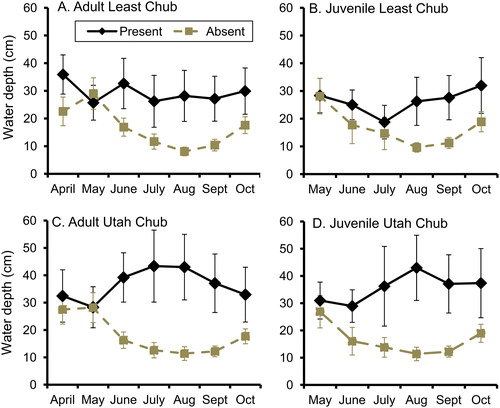
Table 2. Numbers of visual monitoring sites at springs and ponds in which juvenile Least Chub, adult Least Chub, juvenile Utah Chub, and adult Utah Chub were detected during visual surveys from April through October of 2013. There were 50 monitoring sites in all, 23 in springs and 27 in ponds or lentic marsh habitat, of which 40 (19 in springs and 21 in ponds) were used by fish at least once during the visual monitoring surveys.

	Least Chub				Utah Chub
	Juveniles		Adults		Juveniles		Adults
	Springs	Ponds	Springs	Ponds	Springs	Ponds	Springs	Ponds
4 April	0	0	8	16	0	0	5	11
23 May	3	16	5	7	2	14	6	4
20 June	11	20	13	4	8	16	10	3
26 July	13	15	13	5	6	1	7	0
21 August	15	5	14	4	7	1	7	1
13 September	16	5	15	6	9	3	9	3
21 October	14	5	14	5	7	2	12	3

During the overwintering period, significant differences in water temperature between springheads, spring channels, and ponds were evident (ANOVA: F_{2, 62} = 15.52, P < 0.001), with springheads averaging 10.2 °C (95% CI 9.5–10.8 °C, n = 43), channels averaging 7.8 °C (95% CI 5.8–9.7 °C, n = 12) and ice-free pond environments averaging 5.1 °C (95% CI 2.6–7.5 °C, n = 10). During the spawning period, these differences largely disappeared (ANOVA: F_{2, 77} = 1.537, P = 0.221), with water temperatures at springheads averaging 14.6 °C (95% CI 13.5–15.7 °C, n = 29), compared to 12.7 °C in channels (95% CI 9.4–16.0 °C, n = 7) and 13.2 °C in ponds (95% CI 12.1–14.3 °C, n = 44). Differences reemerged during the relatively dry and warm post-spawning period (ANOVA: F_{2, 139} = 7.535, P < 0.001) when ponds had the highest average temperature at 18.7 °C (95% CI 16.8–20.7 °C, n = 29), followed by channels at 17.3 °C (95% CI 15.9–18.7 °C, n = 38) and springheads at 15.2 °C (95% CI 14.3–16.1 °C, n = 75).

Surface water monitoring during 2012–2014 revealed that portions of the spring complex that were inhabited by fish became seasonally fragmented into eight isolated to semi-isolated regions (Figure 5). The four regions of aquatic habitat in the southwestern portion of the spring complex became entirely disconnected from one another, whereas regions of aquatic habitat or clusters of springs in the northeast portion of the spring complex retained some level of connectivity in the form of channels or subsurface connections, but a combination of shallow water and dense emergent vegetation restricted movement of fish through channels connecting these regions. One of the two largest regions of breeding and juvenile habitat in the spring complex (Teal Pond) became fishless during August and September of 2013 and 2014 because resident fish migrated elsewhere before connections to two major springs (Grand Central Spring and Chub Haven Spring) were lost as the pond receded. The other seven regions contained one or more patches of habitat inhabited by Least Chub and Utah Chub throughout 2012–2014, although groups of fish belonging to both species became further isolated in a few of the disconnected springs and small ponds within the four regions to the north of Teal Pond when groundwater and surface water levels were at their lowest. This pattern of habitat fragmentation was accompanied by substantial reductions in the combined surface area of the bodies of water inhabited by each species (Table 3). Least Chub and Utah Chub used a smaller percentage of the available aquatic habitat during the onset of the reproductive season in April and May, when they were concentrated at spawning sites, than during summer months. The populations of both species expanded in their distributions and used most of the available aquatic habitat as water levels rose and habitat fragmentation decreased during October.

Figure 5. Isoline map of the Leland Harris Spring Complex based on water level measurements at surface water monitoring points and corresponding estimates of surface water depths at 3852 bathymetry points during 21 August 2013. Regions of the spring complex that became isolated, or in which movement of fish to and from other regions was greatly restricted, are labelled. Dashed lines indicate boundaries between adjacent regions.

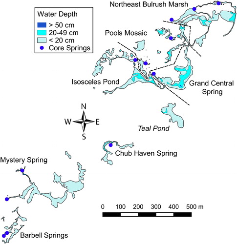
Table 3. The number of isolated bodies of water (patches) occupied by Least Chub and by Utah Chub, the estimated combined surface area of the bodies of water inhabited by each species, and the percentage of the inundated area of the spring complex represented by these bodies of water (%) during visual monitoring surveys from April through October of 2013.

	Least Chub			Utah Chub
Date	Patches	Area (ha)	%	Patches	Area (ha)	%
4 April	2	24.5	74.7	3	23.5	71.6
23 May	2	23.9	72.2	3	22.9	69.2
20 June	6	19.3	92.3	7	18.2	87.1
26 July	9	12.3	94.6	10	10.3	79.2
21 August	10	7.6	83.5	11	6.4	70.3
13 September	9	14.3	90.5	9	13.1	82.9
21 October	5	21.7	95.6	6	20.6	90.7

Population monitoring data indicated that adult Least Chub and especially adult Utah Chub were associated with relatively deep areas within the bodies of water they occupied during August-September of 2013 and 2014, but juvenile Least Chub exhibited no such tendency and the tendency was weak and inconsistent among juvenile Utah Chub (Table 4). Minnow traps containing adult Utah Chub were set 26 cm deeper, on average, than traps that failed to capture adult Utah Chub during 2013, and averaged 17 cm deeper than traps that failed to capture adult Utah Chub in 2014. A similar but less pronounced pattern was evident among adult Least Chub, which were captured in traps set an average of 7 cm deeper than traps that failed to capture adult Least Chub during both 2013 and 2014. The tendency for adults to be captured in traps set in relatively deep water was significant for both species during both years. By contrast, traps that captured juvenile Least Chub were set at depths that did not differ significantly from those of traps that failed to capture juvenile Least Chub during both 2013 and 2014. Traps that captured juvenile Utah Chub were set 3–5 cm deeper, on average, than traps in which no juvenile Utah Chub were captured during 2013–2014, a difference that was marginally significant (Table 4).

Table 4. Comparison of water depths (mean, median, and 25–75% quartile range) at locations of traps in which individuals were present compared to traps in which they were absent for juvenile Least Chub, adult Least Chub, juvenile Utah Chub, and adult Utah Chub during 2013 and 2014 monitoring surveys. The Mann-Whitney U-test statistic and P-values are also shown for each comparison.

Least Chub	2013				2014
	Juveniles		Adults		Juveniles		Adults
	Present	Absent	Present	Absent	Present	Absent	Present	Absent
Mean	29.0	29.8	33.2	26.4	27.7	29.5	32.0	24.7
Median	27	28	30	25	27	27	30	23.5
25–75% QR	20–32	16–35	24–36	15–30	18.5–34	17.5–34.5	23.8–36.5	16–30
n	55	63	52	66	45	49	50	44
	U = 1731		U = 1008		U = 1098		U = 696
	P = 0.996		P < 0.001		P = 0.96		P = 0.002
Utah Chub
Mean	32.8	27.5	49.8	23.6	30.2	27.5	42.4	25.2
Median	29	25	36	24	29	27	34.5	25
25–75% QR	20–37	18–30	30.5–55	17–29.5	22–37.3	16–32.8	32.5–45	16–30.8
n	37	81	25	93	34	60	18	76
	U = 1144.5		U = 284		U = 800		U = 193
	P = 0.04		P < 0.001		P = 0.08		P < 0.001

ANOVAs on TL measurements indicated that there were significant differences in sizes of juvenile Least Chub in different regions of the spring complex during 2012 (F_{5, 370} = 21.31, P < 0.001), 2013 (F_{5, 1324} = 55.70, P < 0.001), and 2014 (F_{5, 762} = 96.55, P < 0.001). Juveniles were smaller at Chub Haven Spring than in other regions during all 3 years, but no other consistent juvenile size differences were evident (Table 5). Adult Least Chub in different regions also differed significantly in size during 2012 (F_{6, 1364} = 92.66, P < 0.001), 2013 (F_{6, 1904} = 273.70, P < 0.001), and 2014 (F_{6, 1585} = 68.45, P < 0.001), and were consistently larger in Barbell Springs than elsewhere, primarily because of a relatively high proportion of adults measuring > 50 mm TL. Barbell Springs was unusual in that the marsh habitat at the southwestern end of the spring complex into which it drains was characterized by consistently shallow water (< 20 cm deep) even during times when relatively large areas of pond habitat with depths > 50 cm were present in the other regions of the spring complex (Figure 1). No Least Chub or Utah Chub were observed or captured in the shallow marsh habitat in the Barbell Springs region, suggesting that it was not used for spawning or as juvenile habitat. In addition, Utah Chub were rare and juvenile Least Chub made up a small proportion of the individuals captured at Barbell Springs during 2012–2014, with no juveniles present in the sample of 213 Least Chub captured there in 2013 (Table 5).

Table 5. The mean and range of total length (TL) measurements of juvenile and adult Least Chub captured and measured in each region of the Leland Harris Spring Complex during August and September of 2012–2014.

Region	Year	Juvenile TL (mm)		Adult TL (mm)		n	% Juv.
		Mean	Range	Mean	Range
Barbell Springs	2012	30.3	28–33	44.0	37–59	143	2.8
	2013	---	---	49.7	34–57	213	0
	2014	27.2	24–31	42.7	32–56	29	20.7
Mystery Spring	2012	30.3	19–33	36.1	33–53	395	26.5
	2013	24.6	17–33	40.4	34–52	331	33.6
	2014	22.7	17–30	40.2	32–54	345	37.4
Chub Haven Spring	2012	24.8	20–30	38.3	32–49	216	30.1
	2013	23.8	17–29	41.1	34–49	427	46.1
	2014	21.8	17–26	38.4	33–48	219	26.0
Isosceles Pond	2012	30.0	25–34	39.8	34–51	70	38.6
	2013	28.1	19–37	39.6	35–47	418	91.9
	2014	22.2	17–32	37.6	34–42	146	36.3
Grand Central Spring	2012	27.7	19–34	38.8	32–51	320	2.3
	2013	25.1	19–32	39.7	34–49	309	17.2
	2014	23.8	20–29	40.5	32–49	276	6.3
Pools Mosaic	2012	27.3	18–35	38.6	34–52	143	40.6
	2013	27.0	15–36	41.5	34–56	734	52.3
	2014	28.1	19–35	40.4	33–51	728	46.2
Northeast Bulrush Marsh	2012	26.9	19–34	37.9	34–52	471	26.5
	2013	27.1	20–33	40.6	35–50	809	24.8
	2014	23.9	18–33	36.8	31–50	558	19.9

The proportion of juveniles among Least Chub captured during population monitoring surveys tended to be highest in the Isosceles Pond and Pools Mosaic regions and lowest in Barbell Springs and Grand Central Spring (Table 6). Observations during trap placement indicated that juveniles were still widely dispersed in relatively stable and permanent pond habitat in the Grand Central Springs region each year during population monitoring, while adults were concentrated at high densities in the springhead and channel, where they were captured in large numbers. This pattern was evident during all 3 years of population monitoring surveys, and resulted in juveniles being underrepresented in samples of Least Chub obtained during population monitoring in the Grand Central Spring region. This was not the case in the Barbell Springs region, where no juveniles were observed or captured outside of the springs during 2012–2014.

Table 6. Total number and number per trap of Least Chub and Utah Chub captured in each region of the Leland Harris Spring complex during population monitoring surveys conducted in August-September of 2012–2014. The mean and range of total length (TL) measurements obtained from Utah Chub that were captured and measured in each region is also given.

Region	Year	Least Chub		Utah Chub		Utah Chub TL (mm)
		n	n/trap	n	n/trap	Mean	Range	n
Barbell Springs	2012	151	11.6	4	0.3	92.5	53–154	4
	2013	214	23.8	4	0.4	54.3	48–61	4
	2014	29	4.8	1	0.2	35.0	35.0	1
Mystery Spring	2012	470	18.8	524	21.0	60.3	32–121	190
	2013	342	17.1	144	7.2	68.9	18–128	144
	2014	594	74.3	100	12.5	33.2	21–87	100
Chub Haven Spring	2012	518	57.6	21	2.3	55.8	37–92	21
	2013	427	53.4	89	11.1	60.6	28–95	89
	2014	804	201.0	9	2.3	39.8	32–70	9
Isosceles Pond	2012	79	4.4	199	11.1	53.4	30–85	169
	2013	418	27.9	4	0.3	43.5	39–55	4
	2014	153	11.8	29	2.2	37.3	27–45	29
Grand Central Spring	2012	486	28.6	120	7.1	59.9	28–102	117
	2013	842	38.3	233	10.6	54.8	22–106	171
	2014	974	81.2	56	4.7	65.8	30–103	56
Pools Mosaic	2012	189	3.9	246	5.0	58.4	34–105	246
	2013	735	23.7	56	1.8	55.5	25–87	53
	2014	754	19.3	291	7.5	45.6	30–78	245
Northeast Bulrush Marsh	2012	741	29.6	59	2.4	50.4	18–80	59
	2013	809	62.2	72	5.5	73.0	29–151	72
	2014	1091	90.2	44	3.7	77.5	52–140	44

Juvenile Least Chub were present in five relatively stable ponds of moderate size in the Grand Central Spring, Isosceles Pond, Pools Mosaic, and Northeast Bulrush Marsh regions during all 3 years of population monitoring. Adults were often present in these ponds as well, all but one of which received discharge directly from a large spring through a narrow channel or subterranean tunnel. The four ponds that were close to large source springs were partially to completely ice-free even during January 2013, when ambient temperatures ranged from −19.4 to −12.8 °C during monitoring activities, and served as overwintering habitat for Least Chub and Utah Chub. The springs that supplied water to these ponds had winter water temperatures ranging from 8.2 to 11.4 °C.

Juvenile Utah Chub were present in all regions of the spring complex during each year, although YOY juveniles were probably lacking in the sample of 42 individuals from the Northeast Bulrush Marsh region in 2014. Very few Utah Chub were captured in Barbell Springs, which precluded any evaluations of size ranges of individuals in that region. In other regions, size ranges of Utah Chub tended to vary from year to year, with the Grand Central Spring region being an exception (Table 5). Adults larger than 100 mm TL were usually associated with springheads, and the largest adults captured during 2013 and 2014 came from a small spring in the Northeast Bulrush Marsh region in which no Least Chub or juveniles were captured and the only connection to other aquatic habitats was subterranean.

Discussion

Data collected during 2012–2014 strongly supported the hypothesis that groundwater plays the primary role in determining the amount of habitat, the degree of habitat fragmentation, and the availability of suitable spawning and juvenile habitats used by Least Chub and Utah Chub in the Leland Harris Spring Complex. GWLs near the spring complex explained 97% of the temporal variation in surface water levels, a 40 cm reduction in the GWL that occurred between February and August of 2013 was accompanied by the loss of most of the surface water in the spring complex (81% by volume), and the populations of Least Chub and Utah Chub became extensively subdivided when GWLs were at their lowest. Adults of both species were usually associated with relatively deep bodies of water and exhibited a tendency to use the deeper portions of the bodies of water in which they were found during population monitoring surveys conducted in late summer and early fall. The 51% reduction in mean surface water depths that occured between February and August of 2013 indicated that the amount and quality of deep-water habitat in the spring complex depended on GWLs.

Surface water levels in ponds fluctuated roughly twice as much as surface water levels in springs in response to changing GWLs. The expansion of large ponds during the winter and early spring provided most of the spawning and juvenile in the spring complex. The relatively warm and productive environments in seasonally inundated pond environments during the late spring and early summer may favor high juvenile growth rates and enhance juvenile recruitment. However, extensive contraction of large ponds that receive input from multiple springs occurred when GWLs were low during late summer and early fall, necessitating a shift in the distribution of juveniles to core spring habitats.

Fragmentation of aquatic habitat at the Leland Harris Spring Complex is a seasonal phenomenon, but populations of Least Chub and Utah Chub experienced some degree of more persistent subdivision caused by habitat fragmentation throughout 2012–2014. Least Chub and Utah Chub at the extreme southwestern end of the spring complex appeared to be largely restricted to Barbell Springs. In addition, an isolated pond (referred to as Doughnut Pond in Grover 2016) fringed by three small springs in the Pools Mosaic region supported a small subpopulation of Utah Chub, but was never connected to adjacent bodies of water during the study period. The consequences of long term habitat fragmentation are difficult to predict, but demographic differences between groups of Least Chub that were temporarily isolated in different regions of the spring complex during 2012–2014 indicate that connectivity between deep springs and ponds of adequate size and depth to serve as spawning and juvenile habitat during the spring and early summer is critical for juvenile recruitment.

The subpopulation of Least Chub in the Barbell Springs region experienced conditions during 2012–2014 that were similar to conditions that would be expected in other regions of the spring complex if long-term reductions in GWLs occur. Population monitoring data indicated that there were relatively few juveniles and a high relative abundance of large adults at Barbell Springs. The two large interconnected springheads that form Barbell Springs exceeded 350 cm in depth and provided stable overwintering habitat, but lacked direct connections to seasonally deep and expansive ponds that were favored as spawning and juvenile habitat elsewhere in the spring complex.

The Chub Haven Spring region became seasonally disconnected from the rest of the spring complex each year during 2012–2014, but had fundamentally different habitat characteristics than Barbell Springs in that it provided direct access to a substantial amount of suitable breeding and juvenile habitat. The region consisted of a deep spring (Chub Haven Spring) that drained through two separate channels into a nearby pond that had connections to two much larger ponds in other regions of the spring complex when spring discharge rates were high enough to fill these ponds (Figures 1 and 5). This allowed unimpeded migration of Least Chub and Utah Chub to and from other regions of the spring complex while these connections existed. Large numbers of Least Chub migrated to Chub Haven Spring each year as ponds receded during late summer; and the average number of Least Chub captured per trap during population monitoring was far higher there than in any other region during 2012 and 2014, and second only to the Northeast Bulrush Marsh region in 2013 (Table 6). The number of individuals captured per trap is a measure of catch per unit effort (CPUE), which may or may not be directly related to population density. However, the high CPUE at Chub Haven Springs during 2012–2014 indicates that large numbers of individuals were present there during populations monitoring each year, and the consistently small sizes of juvenile Least Chub at Chub Haven Spring, compared to other regions of the spring complex, suggests that low per-capita resource availability caused reduced juvenile growth rates.

Most of the variation in GWLs documented in the vicinity of the Leland Harris Spring Complex during 2009–2017 was seasonal in nature and could be attributed to annual cycles in evapotranspiration rates. A pattern of annual fluctuations in shallow GWLs in response to seasonal cycles in evapotranspiration has been observed elsewhere in Snake Valley, as well as other regions of the Great Basin (Welch et al. 2007; Gardner and Heilweil 2014; Hurlow and Kirby 2014). Recent trends toward increasing temperatures and decreased snowpack in the Great Basin and other regions of western North America have the potential to reduce shallow GWLs and spring discharge rates by increasing evapotranspiration and reducing runoff and groundwater recharge (Weissinger et al. 2016; Udall and Overpeck 2017; Devitt et al. 2018). The influence of increased evapotranspiration at the Leland Harris Spring Complex due to warmer temperatures is likely to be minimal during winter, when water loss caused by evapotranspiration is negligible, but would be expected to accelerate the contraction of ponds during late spring and summer and could potentially impact core spring habitats as well.

Negative impacts to groundwater-dependent ecosystems resulting from groundwater removal have already been documented in the Snake Valley, but have yet to occur on a significant scale at the Leland Harris Spring Complex, which is in a relatively remote location. Elsewhere in Snake Valley, GWLs are generally declining due to existing agricultural withdrawals, and simulation modeling of groundwater movement predicts partial to complete loss of spring discharge at several locations under a variety of scenarios related to the number of pending applications for groundwater withdrawal that are ultimately approved (Masbruch and Brooks 2017). Two applications to pump groundwater from sites within 8 km of the Leland Harris Spring Complex for local agricultural use specify annual allocations predicted to result in a 35 cm reduction in shallow GWLs within 5 years, according to simulation modeling in Masbruch et al. (2016). A decline of this magnitude would greatly reduce the amount of spawning and juvenile habitat available to Least Chub and Utah Chub during spring and early summer, creating conditions similar to those that restrict fish to deep springs and a few associated pools during late summer (Figure 5). During late summer and early fall, the additive effects of groundwater removal and high evapotranspiration rates would be expected to entirely eliminate most of the large ponds and perhaps some of the springs, assuming that the relationship between groundwater and surface water levels remains the same as the aquifer is depleted. Plans to minimize these impacts include restricting pumping when GWLs in monitoring wells reach a certain threshold. However, lag times between withdrawal and observed declines limit the effectiveness of this approach (Currell 2016). Consequently, groundwater removal is likely to cause lasting ecological impacts before resultant changes in GWLs can be accurately quantified.

The Southern Nevada Water Authority’s original proposal for large-scale groundwater removal in Snake Valley included withdrawals of up to 62,513,000 m³ per year from the Nevada portion of Snake Valley and additional withdrawals of up to 112,548,000 m³ per year from shallow and deep aquifers in Spring Valley (Hurlow 2014). Plans for the project are evolving, and may ultimately exclude Snake Valley in favor of greater dependence on Spring Valley. However, the potential for substantial groundwater reductions in Snake Valley would still exist because there is a west to east flow-path from the southern portion of the deep carbonate-rock aquifer beneath Spring Valley to the deep carbonate-rock aquifer beneath Snake Valley (Welch et al. 2007; Masbruch et al. 2016). Thus, impacts to the springs and marsh ecosystems of Snake Valley could result from local agricultural withdrawals of groundwater and from large-scale removal and pumping of groundwater to urban areas.

Least Chub are fractional spawners that reproduce during their first year, have a lifespan of up to 6 years, and exhibit the life-history characteristics of an opportunistic species capable of thriving in fluctuating environments and rapidly colonizing newly available habitats (Crawford 1979; Mills et al. 2004; Winemiller 2005). A positive relationship between population density and spring discharge may be a general trend among spring-associated fishes adapted to variable environments (Craig et al. 2016), and periods when spring-fed bodies of water increase in volume and connectivity provide periodic opportunities for fish populations in spring systems to increase in abundance and distribution. Utah Chub have longer generation times than Least Chub, which may limit the ability of Utah Chub populations to increase rapidly in response to brief periods of favorable environmental conditions, but exhibit a remarkable degree of life-history plasticity that facilitates adaptation to variable environments (Johnson 2002). At the Leland Harris Spring Complex, individuals of both species require core spring environments to survive extreme conditions, but rely on more variable and often transient pond environments for reproduction and juvenile recruitment. Relatively stable refugia, such as core springs, are necessary for the persistence of populations of fish adapted to ecosystems subject to contraction and extreme conditions during dry periods, and opportunistic migration to and from these refugia can be critical to the resilience of these populations (Magoulick and Kobza 2003).

During periods of high GWLs and spring discharge rates at the Leland Harris Spring Complex, such as the one that occurred in the late winter and spring of 2013, surface water levels are high enough to allow mixing of individuals from different regions, increase the amount of spawning and juvenile habitat, and facilitate colonization of bodies of water that are usually isolated. In light of these fluctuations and the natural resiliency of Least Chub and Utah Chub populations, future impacts of reductions in GWLs that occur as a result of groundwater withdrawal and/or climate change could be partially offset by occasional periods of rebounding GWLs, but this would require a greater capacity for rapid recharge than may currently exist in the system and would become increasingly unlikely if core spring habitats are impacted.

Acknowledgments

Thanks to Tiffanee Hutton and Danielle Voisin for assistance with bathymetric surveys and GPS mapping of surface waters at the Leland Harris Spring Complex during 2013–2014. Thanks especially to Ed Alder for providing access to his property, which encompasses the northeastern half of the Leland Harris Spring Complex, and for many years of cooperation with monitoring and management efforts. Rich Emerson provided valuable data from groundwater monitoring and LIDAR mapping of surface elevations conducted by the Utah Geological Survey.

Disclosure statement

No potential conflict of interest was reported by the author.

Funding

This project was funded through a grant (F12AP00521) from the U.S. Fish and Wildlife Service and by additional funding from the U.S. Bureau of Land Management, Utah Endangered Species Mitigation Fund, and State Wildlife Grants received by the Utah Division of Wildlife Resources.

Data availability

The data collected and analyzed in this study is accessible to the public under the DOI: 10.6084/mp.figshare.7121699.

Additional information

Notes on contributors

Mark C. Grover

Mark C. Grover is an aquatic ecologist whose research interests include landscape ecology and conservation biology. He currently works as the Colorado River Basin Native Aquatics Coordinator for the Arizona Game and Fish Department.

References

- Craig CA, Kollaus KA, Behen KPK, Bonner TH. 2016. Relationships among spring flow, habitats, and fishes within evolutionary refugia of the Edwards Plateau. Ecosphere. 7(2):e01205.
- Crawford M. 1979. Reproductive modes of the least chub Iotichthys phlegethontis Cope. M.S. Thesis. Logan (UT): Utah State University.
- Currell MJ. 2016. Drawdown “triggers”: a misguided strategy for protecting groundwater-fed springs and streams. Groundwater. 54(5):619–622.
- Currey DR. 1990. Quaternary palaeolakes in the evolution of semidesert basins, with special emphasis on Lake Bonneville and the Great Basin, U.S.A. Palaeogeogr Palaeoclimatol Palaeocol. 76(3-4):189–214.
- Deacon JE, Williams AE, Williams CD, Williams JE. 2007. Fueling population growth in Las Vegas: how large-scale groundwater withdrawal could burn regional biodiversity. Bioscience. 57(8):688–698.
- Devitt D, Bird B, Lyles B, Fenstermaker L, Jasoni R, Strachan S, Arnone JIII, Biondi F, Mensing S, Saito L. 2018. Assessing near surface hydrologic processes and plant responses over a 1600 m mountain valley gradient in the Great Basin, NV, USA. Water. 10(4):420. doi.10.3990/w10040420.
- Estabrook GF, Smith GR, Dowling TE. 2007. Body mass and temperature influence rates of mitochondrial DNA evolution in North American cyprinid fish. Evolution. 61(5):1176–1187.
- Gardner PM, Heilweil VM. 2014. A multi-tracer approach to understanding regional groundwater in the Snake Valley area of the eastern Great Basin, USA. Appl Geochem. 45:33–49.
- Grover MC. 2016. Relationships of groundwater levels to surface water fluctuations and habitat associations of Least Chub (Iotichthys phlegethontis) in a Great Basin Spring Complex. In: Comer JB, Inkenbrandt PC, Krahulec KA, and Pinnell ML, editors. Resources and geology of Utah’s West Desert. Utah: Utah Geological Association Publication 45; p. 247–272.
- Hargreaves GH, Samani ZA. 1985. Reference crop evapotranspiration from temperature. Appl Eng Agric. 1:96–99.
- Houston DD, Shiozawa DK, Riddle BR. 2010. Phylogenetic relationships of the western North American cyprinid genus Richardsonius, with an overview of phylogeographic structure. Mol Phylogenet Evol. 55(1):259–273.
- Hubbs CL, Miller RR, Hubbs LC. 1974. Hydrographic history and relict fishes of the north-central Great Basin. Memoirs of the California Academy of Sciences. San Francisco: California Academy of Sciences; vol. 7; p. 1–257.
- Hurlow H. 2014. Introduction. In: Hurlow H, editor. Hydrogeologic studies and groundwater monitoring in Snake Valley and adjacent hydrographic areas, west-central Utah and east-central Nevada. Utah: Utah Geological Survey Bulletin 135; p 1–17.
- Hurlow H, Kirby S. 2014. Evaluation of groundwater flow paths in Snake Valley and adjacent hydrographic areas. In: Hurlow H, editor. Hydrogeologic studies and groundwater monitoring in Snake Valley and adjacent hydrographic areas, west-central Utah and east-central Nevada. Utah: Utah Geological Survey Bulletin 135; p. 233–256.
- Johnson JB. 2002. Evolution after the flood: phylogeography of the desert fish Utah Chub. Evolution. 56(5):948–960.
- Magoulick DD, Kobza RM. 2003. The role of refugia for fishes during drought: a review and synthesis. Freshwater Biol. 48(7):1186–1198.
- Masbruch MD, Gardner PM, Brooks LE. 2016. Numerical simulation of groundwater movement and heat transport in Snake Valley and surrounding areas, Juab, Millard, and Beaver counties, Utah, and White Pine and Lincoln counties, Nevada. In: Comer JB, Inkenbrandt PC, Krahulec KA, and Pinnell ML, editors. Resources and geology of Utah’s West Desert. Utah: Utah Geological Association Publication 45; p. 201–220.
- Masbruch MD, Brooks LE. 2017. Potential effects of existing and proposed groundwater withdrawals on water levels and natural groundwater discharge in Snake Valley and surrounding areas, Utah and Nevada. U.S. Geological Survey Open-file Report 2017-1026. Available from https://doi.org/10.3133/ofr20171026.
- Mills MD, Belk MC, Rader RB, Brown JE. 2004. Age and growth of least chub, Iotichthys phlegethontis, in wild populations. West N Am Nat. 64(3):409–412.
- Oviatt CG. 1997. Lake Bonneville fluctuations and global climate change. Geology. 25(2):155–158.
- Patten DT, Rouse L, Stromberg JC. 2008. Isolated spring wetlands in the Great Basin and Mojave Deserts, USA: potential response of vegetation to groundwater withdrawal. Environ Manag. 41(3):398–413.
- Rees HD. 1935. The feeding habitat of the chub, Tigoma atraria. M.S. Thesis. Logan (UT): Utah State University.
- Sada DW, Vinyard GL. 2002. Anthropogenic changes in historical biogeography of Great Basin aquatic biota. In: Great Basin aquatic systems history. Smithsonian Contributions to the Earth Sciences, 33. Washington, DC: Smithsonian Institution Press. p. 277–293.
- Sigler WF, Sigler JW. 1987. Fishes of the Great Basin: a natural history. Reno: University of Nevada Press.
- Smith GR, Dowling TE, Gobalet KW, Lugaski T, Shiozawa DK, Evans RP. 2002. Biogeography and timing of evolutionary events among Great Basin fishes. In: Hershler R, Madsen DB, and Currey DR, editors. Great Basin aquatic systems history. Smithsonian Contributions to Earth Sciences, no. 33 Washington, DC: Smithsonian Institution Press. p. 175–234.
- Smith GR, Badgley C, Eiting TP, Larson PS. 2010. Species diversity gradients in relation to geological history in North American freshwater fishes. Evolut Ecol Res. 12:693–726.
- Udall B, Overpeck J. 2017. The twenty-first century Colorado River hot drought and implications for the future. Water Resour Res. 53(3):2404–2418.
- United States Fish and Wildlife Service. 2014. Endangered and threatened wildlife and plants; 12-month finding on the petition to list least chub as an endangered or threatened species. Federal Register. 79(165):51042–51065.
- Weissinger R, Philippi TE, Thoma D. 2016. Linking climate to changing discharge at springs in Arches National Park, Utah, USA. Ecosphere. 7(10):e01491.
- Welch AH, Bright DJ, Knochenmus LA. 2007. Water resources of the Basin and Range carbonate-rock aquifer system, White Pine County, Nevada, and adjacent areas in Nevada and Utah. US Geological Survey Scientific Investigations Report 2007-5261.
- Williams TJ, Johnson JB, Belk MC. 2017. Interaction between predation environment and diet constrains body shape in Utah chub, Gila atraria (Cypriniformes: Cyprinidae). Biol J Linn Soc. 122(1):147–156.
- Winemiller KO. 2005. Life history strategies, population regulation, and implications for fisheries management. Can J Fish Aquat Sci. 62(4):872–885.