Threshold temperature constraints on reproduction of the banded killifish (Fundulus diaphanus)

Abstract

Banded killifish (Fundulus diaphanus) are a small, freshwater fish that have a wide distribution in eastern North America and are considered a species-at-risk on the island of Newfoundland. We posit that because Newfoundland’s summer climate is much cooler than other locations at similar latitudes, there may be different constraints on banded killifish reproduction. We measured embryonic development under four temperatures (10, 16, 22, and 28 °C) and two conductivities (0.6 and 1.2 mS/cm). Warmer temperatures led to more developed embryos prior to death in embryos that ultimately did not hatch, higher hatch success, faster hatch time, and fewer thermal units to hatch. Conductivity and temperature interacted to affect hatch size. Therefore, banded killifish are likely challenged by the low temperature and conductivity conditions in Newfoundland which may result in reproductive constraints, and perhaps complete cohort failures in relatively cool summers.

Keywords:

• Compensatory development
• thermal adaptation
• degree days
• range edge

Introduction

Species’ distributions are limited by physical barriers such as lake edges that create a border preventing individuals from dispersing, and both biotic and abiotic environmental barriers (Hardie and Hutchings 2010) that generally slow rather than fully stop dispersal (Goldberg and Lande 2007). Temperature generally limits species distributions, particularly for ectotherms. However, seasonality, weather, and microclimate make specific temperature effects hard to predict. Thermal optimum and tolerance thresholds affect distribution, survival, growth, and reproduction (Johnson and Kelsch 1998). These thresholds are influenced by local adaptation, acclimation, and life history stage.

Within individuals, there are differences in thermal tolerance through ontogeny. Young offspring have narrower tolerance and optima ranges than adults; therefore, reproduction presents extra challenges at the edges of species ranges. For example, brown trout adults can tolerate up to 28 °C (Carline and Machung 2001), but their thermal tolerance is lower in earlier life stages: parr and smolt can survive to 26 °C, hatchlings to 24 °C, but embryos can only tolerate to 13 °C (Elliott and Elliott 2010). As a result, many species have temperature-phenology breeding plasticity (flexible reproductive timing) as an adaptation to coincide reproduction with more optimal temperatures (Bowler and Terblanche 2008). Breeding phenology can be adaptive in areas where there is a strong seasonal time constraint that is often seen at northern or southern range edges (Rowe and Ludwig 1991; Edge et al. 2017). However, even with such adaptations, temperature can be a limiting factor of a species’ distribution.

Banded killifish (Fundulus diaphanus) have a wide but patchy distribution across eastern North America. Fundulidae generally spawn in estuaries because their embryos perform better in salinities around 20‰; however, banded killifish spawn in warm, freshwater (Fritz and Garside 1974) despite adults being able to survive salinities higher than seawater (Griffith 1974). Their distributional range includes much of the eastern United States and Canada, as far south as South Carolina, to the northeastern edge of Atlantic Canada, including the island of Newfoundland (April and Turgeon 2006). Newfoundland’s climate is not well predicted by latitude because spring and summer conditions are much cooler than typical. Additionally, banded killifish have a relatively high conductivity tolerance compared to other freshwater fish (April and Turgeon 2006), but conductivity is relatively low in Newfoundland watersheds (Department of Environment and Conservation, 2015, n.d.). In fishes, both water chemistry and temperature affect many parts of life history, including size at maturity, growth rate (Schultz et al. 1996), and reproductive factors, such as hatch time (Wilson and Hubbs 1972; Pepin 1991; DiMichele and Westerman 1997; Gillooly et al. 2002; Penney et al. 2018) and hatch size (Brown et al. 2011; Penney et al. 2018).

Despite the cited concerns over the survival of Newfoundland’s peripheral killifish populations (Osborne and Brazil 2006; COSEWIC 2014), there is a dearth of information regarding their early life history. Continental populations begin spawning in April and May but Newfoundland populations do not begin until June or July (Mitchell and Purchase 2014). It is unknown whether cool temperatures cause additional constraints or if low conductivities compound impacts on embryonic development. The objective of this paper was to determine how embryonic development is affected by multiple conditions (temperature and conductivity; manipulated in the laboratory) that banded killifish experience at their range edge. We tested the hypotheses that 1) temperature has a strong effect and predicted that fish have higher hatch success, faster time to hatch (Schaefer 2012), and larger size at hatch in warmer temperatures (Brown et al. 2011); and 2) that conductivity causes additive impacts, with a prediction that the embryos have higher hatch success and larger size at hatch under higher conductivity (Brown et al. 2012).

Materials and methods

The care and use of experimental animals was in accordance with Memorial University of Newfoundland’s animal care committee (Protocol number 12-04-cp) and the Department of Fisheries and Oceans collection permit (#NL-2260-14).

Temperature data

Spring warming of freshwater is impacted by air temperature, solar radiation, water source, water body size, and flow rate. To examine differences in water temperature between Newfoundland and neighboring Maritime killifish populations, ideally we would have data on similar sized lakes representing appropriate habitat. However, the only detailed data we could retrieve were air temperatures from historical Environment Canada records (http://climate.weather.gc.ca). We used data from 2010 to 2017 at seven sites in Newfoundland and eight sites in the Maritimes (New Brunswick and Nova Scotia). We restricted comparisons to the banded killifish's potential growing season (1 April to 31 October; Chippett 2004; Figure 1(a)) and calculated the thermal summed units when the temperature was over 15 °C for the daily average for each area (Figure 1(b), see Supplementary material Appendix Table A1).

Figure 1. (a) Temperature comparisons and (b) thermal summed units (when over 15 °C) from weather stations in Newfoundland (grey, n = 7) and the Maritimes (black, n = 8) from April to the end of October (average temperature from all stations for 2010 to 2017). Newfoundland has approximately 2/3rds of the accumulated thermal units as the Maritimes. (Note: grey shows standard deviation among stations in A and for B is negligible at this scale, so does not appear on this graph).

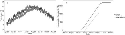
Table 1. A summary of analyses of deviance on the fixed effects – embryo size (size), temperature (temp), conductivity (cond), and a temperature × conductivity interaction, from general linear models (GLM) for hatch success (proportion), hatch time (accumulated thermal units, °C), and hatch size (length in mm). χ² values, degrees of freedom, and the corresponding p value, are given for each effect.

	Hatch success			Stage reached			Hatch time			Hatch size
Factor	df	χ^2	p	df	χ^2	p	df	χ^2	p	df	χ^2	p
Size	1	2.68	0.10	1	4.59	0.03*	1	2.63	0.10	1	0.53	0.47
Temp	3	72.12	0.001***	3	46.66	0.001***	2	226.56	0.001***	2	23.20	0.001***
Cond	1	0.003	0.95	1	0.78	0.38	1	3.14	0.08	1	2.82	0.09
Size × Cond	1	0.02	0.88	1	0.002	0.96	1	2.21	0.14	1	1.11	0.29
Size × Temp	3	0.20	0.98	3	5.44	0.14	2	22.40	0.001***	2	1.23	0.54
Temp × Cond	3	3.02	0.39	3	3.84	0.28	1	2.32	0.14	1	13.64	0.002***

Population and collection information

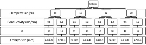
We collected banded killifish embryos from Burton’s Pond in St. John’s, NL, Canada (47.574°N, 52.728°W). This population was introduced in 1999 (Mitchell and Purchase 2014) from Indian Bay, NL (COSEWIC 2014). Embryos were collected on artificial (yarn, ∼10- to 15-cm-long threads) spawning mops (∼20), which were used to mimic the plant substrate that banded killifish eggs typically adhere to. The mops were checked twice daily. Embryos stripped from the mops during the first collection were not used because fertilization time (within 20 h) was unknown. The second collection took place 4 h later, and therefore, embryos were known to be within the first 4 h of development. Individual embryos were fully immersed in water in Petri dishes placed in incubators at their respective temperatures, and the water was topped up daily. Each individual embryo was checked under a dissecting microscope for cell division to ensure fertilization, and embryos from each collection day were distributed evenly into the different treatments (Figure 2). The majority of the embryos were collected between 27 June and 1 July (n = 84). Because of low hatch success at the lower temperatures, we collected additional embryos (n = 23; between 9 and 11 July) and added them evenly into the 10 and 16 °C levels to increase the sample size.

Figure 2. The number of embryos and the mean embryo size (standard deviation) for the temperature and conductivity treatments.

Experimental design

A 4 × 2 experimental design was used (Figure 2), where embryos were sorted into four temperatures (10, 16, 22, and 28 °C) and two conductivities (0.6 and 1.2 mS/cm) that allowed us to examine the possibility of an interaction. Temperatures were chosen based on the documented thermal range for spawning 19–24 °C (Chippett 2004) and included summer temperatures typical of Newfoundland (10, 16 °C; Figure 1(a)) and elsewhere in the banded killifish’s range (22, 28 °C). The two conductivities were representative of those typical of Newfoundland’s freshwater systems (Department of Environment and Conservation 2015). Water conductivities were prepared using sea salt (Instant Ocean Spectrum Brands, Blacksburg, VA, USA) and deionized water.

Development and size metrics

Every 12 h from collection to hatch or death, each individual embryo was photographed in its Petri dish using a stage microscope (Leica M80, Wetzlar, Germany). Petri dishes with embryos were not out of their incubators for more than 10 min during the photographic process. To our knowledge, no published documentation on embryonic developmental stages of the banded killifish exists; therefore, we compared the development of our embryos to a congeneric species, the common mummichog (Fundulus heteroclitus), as outlined by Armstrong and Child (1965). It was possible to distinguish six stages: cleavage (2–64 cell stage), blastula, gastrula, neuralae, segmentation (further embryo growth and organ development), and hatch (Figure 3). Any embryo that did not develop for seven consecutive days was considered to have ceased development.

Figure 3. Photo examples for different stages of embryonic development of the banded killifish (Fundulus diaphanus). (a) cell division (4 cell stages); (b) blastulae; (c) gastrulae; (d) neurulae; (e) to (g) segmentation (growth, differentiation, and development); (h) newly hatched larva. Stages were based on drawings in Armstrong and Child (1965). The perpendicular lines in panel A indicate how embryo size was determined. Black circles were added in panels A through C to indicate where the cells were. Note: the large round drops are oil globules from the yolk not embryonic cells.

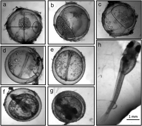
All size measurements were collected from digital photos in ImageJ (Rasband 2018; Schneider et al. 2012). Embryo size was determined from the first photograph on collection day and was measured as the average of two axes of the yolk (the longest and its perpendicular; see Figure 3(a)). Standard length of the larvae on hatch day was used for hatch size.

Data analyses

General approach

All of the figures (using package ‘ggplot2’), data processing and statistics (using packages car, ggpmisc, lme4, multcomp, plyr, and survival) were created and conducted in R version 3.3.3 (R Development Core Team 2015). For all statistical tests, an alpha of 0.05 was used. Assumptions of normality and heteroscedascity were tested using the residuals, and no deviations were observed using a normal error structure (hatch size) and binomial structure (hatch success, developmental stage). The same model parameters (model 1) were run for all of the dependent variables (DVs): last developmental stage reached before development ceased (herein ‘developmental stage’), hatch success, and hatch size. Independent variables included embryo size (S, covariate), temperature (T), conductivity (C), and all possible two-way interactions among the variables. [model 1] $$\text{DV}\sim S+T+C+S\mathrm{\times }T+S\mathrm{\times }C+T\mathrm{\times }C+\text{error}$$[model 1]

We did explore the three-way interactions (S×T×C) for each DV; however, it was only significant for hatch success (p = 0.02). The hatch success pattern was the same for both conductivities (i.e. 22 °C level had the highest and the 10 °C level had the lowest hatch success). So, we elected to split the data to analyze each conductivity level separately, in both models the only significant factor was temperature. Therefore, we did not include the three-way interaction in the final analyses because it did not change any of our conclusions.

Developmental stage reached

For developmental stage reached, the dependent variable was the final developmental stage reached (six stages: cleavage, blastulae, gastrulae, neurulae, segmentation, and hatch); therefore, the data were considered ordinal. To determine whether the temperature and conductivity treatments affected survival to different developmental stages, an ordinal regression was conducted as a Cumulative Link Model (CLM, see Guisan and Harrell 2000 for a similar analysis) on model 1 with an ‘equidistant’ threshold, using the ‘ordinal’ package in R.

Hatch success, time, and size

To determine the impacts of the main effects (model 1) on 1) hatch success – we conducted a generalized linear model (GzLM) with a binomial error structure; then, an analysis of deviance was performed to determine significance; and 2) hatch time and hatch size – we conducted a GzLM with normal error structure; then, an analysis of deviance was performed to determine significance. The 10 °C level had no embryos hatch, and 16 °C only had two embryos hatch; therefore, for hatch time and size, the tests were only on the temperatures with successful hatching. For hatch size, there was a significant interaction between temperature and conductivity; therefore, a Tukey post hoc test was conducted.

Results

Temperature differences

Our eight years of air temperature data showed that Newfoundland warms up later in the season and does not reach the same highs as the Maritimes (Figure 1(a)). There was a difference in accumulated thermal units (Figure 1(b)) with a 15 °C cutoff, which means substantial variation in annual development and growth potential. By the end of October, the Maritimes reached over 1700 °C thermal units, while Newfoundland reached around 1000 °C (ATU, see Supplementary material Appendix Table A1).

Hatch success

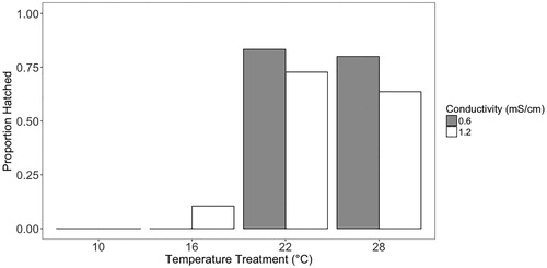
Hatch success was significantly affected by temperature; however, embryo size, conductivity, and the interaction between conductivity and temperature were not significant (Table 1). Neither of the 10 °C levels had embryos hatch, while 22 and 28 °C had reasonable hatch success (>74%), and the two 16 °C treatments had very low hatch success (0% and 10%) (Figure 4).

Figure 4. Hatch proportion for embryos reared at each conductivity and temperature. These are replicate embryos reared individually, not replicate groups; therefore, there are no error bars.

Developmental stage

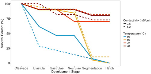
We used a CLM and determined that temperature significantly affected the stage reached by developing embryos, but the effects of embryo size, conductivity, and the interactions between embryo size, conductivity, and temperature were not significant (Table 1). The 22 and 28 °C levels had relatively high hatch success, and those that did not hatch died during all five stages of development (Figure 5). No fish hatched at 10 °C, and the embryos died over all five stages. However, at 16 °C most embryos developed until segmentation, organ growth, and differentiation but did not hatch.

Figure 5. Survival curves through the different stages of embryonic development for each temperature (color) and conductivity (solid or dashed line) treatments.

Hatch time

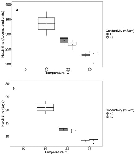
For the individually incubated embryos that did hatch (n = 34), there was a significant interaction (p < 0.001) between embryo size and temperature on time to hatch in accumulated thermal units (Table 1). Embryo size, conductivity, and the interaction between conductivity and temperature were not significant (Figure 6). The embryos in the 28 °C level hatched in the fewest accumulated thermal units and the shortest amount of time (accumulated thermal unit mean: 233.1 ATU, sd: 10.8; days mean: 8.3 sd: 0.4), followed by 22 °C (mean: 274.4 ATU, sd: 12.9; days mean: 12.5 sd: 0.6) and 16 °C (mean: 335.7ATU, sd: 56.6; days mean: 21.0 sd: 3.5). Note: mean and standard deviation were calculated using all individuals at a particular temperature regardless of conductivity.

Figure 6. Hatch time in accumulated thermal units (a) and days (b) for each conductivity and temperature. The box plot shows the interquartile range (IQR, 25% and 75%), and the line shows the median value for hatch time among individuals. Whiskers represent the next quartile (1.5 × IQR), and outliers are represented by the black dots. The open circles represent the mean. Note: no fish hatched at 10 °C in either conductivity, or in the 16 °C–0.6 mS/cm treatment.

Hatch size

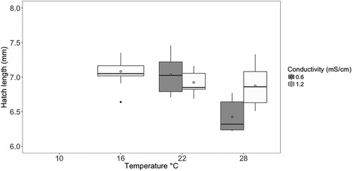
There was a significant interaction between temperature and conductivity on hatch length (Table 1). Initial embryo size was not significantly related to hatch length. Results of the Tukey post hoc test showed that the 0.6 mS/cm conductivity and 28 °C temperature treatment produced significantly smaller larvae (mean: 6.4 mm, sd: 0.2, p < 0.001) at hatch than the other four treatment combinations (mean 7.1 mm, sd:0.2) that resulted in hatchlings (Figure 7).

Figure 7. Hatch length for each conductivity and temperature. Where the box plot shows the interquartile range (IQR, 25% and 75%), and the line is the median value for length. Whiskers represent the next quartile (1.5 × IQR), and outliers are represented by the black dots. The open circles represent the mean. Note: no fish hatched at 10 °C in either conductivity, or in the 16 °C–0.6 mS/cm treatment.

Discussion

Banded killifish likely experience reproductive constraints due to the nature of the abiotic factors in Newfoundland. We found support for our first hypothesis that embryonic development is affected by temperature, where higher temperatures resulted in higher hatch success and less time to hatch. There was a significant interaction between temperature and conductivity on hatch size, with shorter hatchlings at the lowest conductivity and highest temperature. We found no support for our second hypothesis that incubation is affected by conductivity, independent of temperature.

Low experimental temperatures negatively affected banded killifish embryonic development. The lowest temperatures (16 and 10 °C) had little or no hatch success. Temperature significantly affected the stage that the embryos reached before development ceased, where lower temperatures resulted in lower hatch success and the embryos died at less developed stages. Only 10% of embryos reached the neurulae stage at 10 °C compared to ∼75% at 16 °C. If an embryo develops past the neurulae stage to the segmentation and growth phase, it seems they are much more likely to hatch. At 22 and 28 °C, there was high hatch success (at least 74%). These results indicate that there may be a developmental temperature threshold between 16 and 22 °C. This is concerning because our analysis of summer temperatures in Newfoundland showed that across seven locations, from 2010 to 2017 the average daily air temperature never reached 22 °C in Newfoundland (Supplementary material Appendix Table A1).

In fishes, colder temperatures increase the length of incubation, but it is often more efficient (compensatory development) as hatching requires fewer accumulated thermal units (e.g. salmonids Crisp 1988; Atlantic cod Gadus morhua Geffen et al. 2006; European plaice Pleuronectes platessa Ryland and Nichols 1975). In contrast, time to hatch was faster and required fewer accumulated thermal units at warmer temperatures in our killifish experiment. A similar result has also been shown in other Cyprinodontiformes species (striped killifish F. majalis Abraham 1985; desert pupfish Cyrpinodon macularius Kinne and Kinne 1962).

Our results showed that conductivity did not affect developmental stage reached, hatch success, or timing. The only factor that was affected by conductivity was hatch size, as an interaction with temperature. Hatchlings were significantly smaller at the lower conductivity and highest temperature treatment. The overall lack of effect of conductivity on development and survival is somewhat surprising given that previous work has shown that banded killifish had optimal hatch success and growth rates at conductivities three to four times higher than what we tested (Griffith 1974). There are three possible explanations for this result: 1) perhaps there is local adaptation to low conductivity in Newfoundland; 2) conductivity did not have an effect in treatments where temperature was not a stressor (see Penney et al. 2018). In other words, the embryos could cope with the low conductivity in the treatments that approached optimal temperature (22 °C), whereas at 28 °C, the embryos were experiencing stress from both high temperature and low conductivity which has additive energetic costs resulting in smaller embryos; 3) we only tested two conductivities, and both of them were low (0.6 and 1.2 mS/cm). Perhaps if we had tested a wider spectrum of conductivities (e.g. between 1 and 32 mS/cm), we could have obtained a clearer result of conductivity’s effect on development.

Newfoundland’s populations of banded killifish are considered at risk and are currently listed by the province of Newfoundland and Labrador as a vulnerable species (Osborne and Brazil 2006), the Canadian Species at Risk Act as a species of special concern, and the International Union for Conservation of Nature as having a threat impact level of ‘high’ (COSEWIC 2014). We conclude that the reproductive potential of banded killifish is inhibited by poor summer temperatures in Newfoundland. Some years the average daily air temperature never reaches 20 °C, and when it does, it can take until July to do so. In addition to hatching constraints, another temperature limitation with Newfoundland populations is a shift in spawning period to late June to July compared to continental populations which spawn from April to May (Mitchell and Purchase 2014), decreasing their growing season. How this affects juvenile overwinter survival is unknown.

Studying species at their distributional extremes can be informative, particularly for species that may be exposed to multiple suboptimal conditions that may require acclimation (Buckley et al. 2010; Alofs and Jackson 2015). The banded killifish are affected by edge conditions in three ways: 1) shifted spawning phenology due to cool spring temperatures means they have a shorter growing season; 2) the growing season is cold, so there are fewer accumulated thermal units available to use for development; and 3) because they have great difficulty developing when it is 16 °C or colder, they will be challenged in years that Newfoundland has cool summers. These factors may result in additive negative impacts, which may mean reproductive declines and perhaps complete cohort failures in moderately cool years. Despite this, it is possible that Newfoundland banded killifish are locally adapted to reproduce in colder water than elsewhere, but this remains untested. For example, in a congeneric species (mummichog, Fundulus heteroclitus) it has been shown that populations from different latitudes have differences in behavioral thermoregulation (Fangue et al. 2009) and temperature tolerance ranges (Fangue et al. 2006, 2008). As such, special care should be taken to understand whether the Newfoundland populations of banded killifish are adapting to less than optimal conditions in order to help protect these populations.

Notes on contributors

All authors contributed to the conception of the project. HDP and MAL ran the experiment and collected data. HDP conducted the statisitcal analyses, and all authors contributed to the writing and editing process.

Acknowledgements

The authors would like to thank V. Shikon for help in the field, S. Trueman for help with data analysis, and I.A. Fleming, T.E. Van Leeuwen, C. Brown, M. Abrahams, S. Einum, and two anonymous reviewers for comments on an earlier version of the manuscript.

Disclosure statement

The authors report no conflict of interest.

Additional information

Funding

Funding for this project was provided by Memorial University of Newfoundland Undergraduate Funding (Summer Undergraduate Research Award) to MAL, the Natural Sciences and Engineering Research Council of Canada through a graduate scholarship to HDP and a Discovery grant (355507-2008) to CFP, and grants from the Canada Foundation for Innovation (CFI 19360), and the Research and Development Corporation of Newfoundland and Labrador to CFP

.

References

- Abraham BJ. 1985. Species profiles: life histories and environmental requirements of coastal fishes and invertebrates (mid-Atlantic)–Mummichog and striped killifish. U.S. Fish Wildl. Serv. Biol. Rep. 82(11.40). Available from: U.S. Army Corps of Engineers, TR EL-82-4. 23 pp.
- Alofs KM, Jackson DA. 2015. The abiotic and biotic factors limiting establishment of predatory fishes at their expanding northern range boundaries in Ontario, Canada. Glob Change Biol. 21(6):2227–2237.
- April J, Turgeon J. 2006. Phylogeography of the banded killifish (Fundulus diaphanus): glacial races and secondary contact. J Fish Biol. 69(sb):212–228.
- Armstrong PB, Child JS. 1965. Stages in the normal development of Fundulus heteroclitus. Biol Bull. 128(2):143–168.
- Bowler K, Terblanche JS. 2008. Insect thermal tolerance: what is the role of ontogeny, ageing and senescence? Biol Rev Cambridge Philos Soc. 83(3):339–355.
- Brown CA, Galvez F, Green CC. 2012. Embryonic development and metabolic costs in gulf killifish Fundulus grandis exposed to varying environmental salinities. Fish Physiol Biochem. 38(4):1071–1082.
- Brown CA, Gothreaux CT, Green CC. 2011. Effects of temperature and salinity during incubation on hatching and yolk utilization of gulf killifish Fundulus grandis embryos. Aquaculture 315(3–4):335–339.
- Buckley J, Bridle JR, Pomiankowski A. 2010. Novel variation associated with species range expansion. BMC Evol Biol. 10(1):382–383.
- Carline RF, Machung JF. 2001. Critical thermal maxima of wild and domestic strains of trout. Trans Am Fish Soc. 130(6):1211–1216.
- Chippett JD. 2004. An examination of the distribution, habitat and genetic and physical characteristics of Fundulus diaphanus, the banded killifish in Newfoundland and Labrador [master thesis]. Canada: Memorial University of Newfoundland.
- COSEWIC. 2014. COSEWIC assessment and status report on the banded killifish Fundulus diaphanus Newfoundland populations in Canada. Ottawa: Committee on the Status of Endangered Wildlife in Canada. x + 22 pp.
- Crisp DT. 1988. Prediction, from temperature, of eyeing, hatching and ‘swim-up’ times for salmonid embryos. Freshw Biol. 19(1):41–48.
- Department of Environment and Conservation. 2015. Government of Newfoundland and Labrador. Real-Time Water Quality Deployment Report Paddy’s Pond 2015-08-28 to 2015-10-02.
- Department of Environment and Conservation. n.d. Government of Newfoundland and Labrador. Conductivity contours based on Canada-Newfoundland water quality monitoring agreement data. www.Mae.Gov.Nl.ca/Waterres/Quality/Background/Conductivity.Pdf.
- DiMichele L, Westerman ME. 1997. Geographic variation in development rate between populations of the teleost Fundulus heteroclitus. Marine Biol. 128(1):1–7.
- Edge CB, Rollinson N, Brooks RJ, Congdon JD, Iverson JB, Janzen FJ, Litzgus JD. 2017. Phenotypic plasticity of nest timing in a post-glacial landscape: how do reptiles adapt to seasonal time constraints? Ecology 98(2):512–524.
- Elliott JM, Elliott JA. 2010. Temperature requirements of Atlantic Salmon Salmo salar, Brown Trout Salmo trutta and Arctic Charr Salvelinus alpinus: predicting the effects of climate change. J Fish Biol. 77(8):1793–1817.
- Fangue NA, Hofmeister M, Schulte PM. 2006. Intraspecific variation in thermal tolerance and heat shock protein gene expression in common killifish, Fundulus heteroclitus. J Exp Biol. 209(15):2859–2872.
- Fangue NA, Mandic M, Richards JG, Schulte PM. 2008. Swimming performance and energetics as a function of temperature in killifish Fundulus heteroclitus. Physiol Biochem Zool. 81(4):389–401.
- Fangue NA, Podrabsky JE, Crawshaw LI, Schulte PM. 2009. Countergradient variation in temperature preference in populations of killifish Fundulus heteroclitus. Physiol Biochem Zool. 82(6):776–786.
- Fritz ES, Garside ET. 1974. Salinity preferences of Fundulus heteroclitus and F. diaphanus (Pisces: Cyprinodontidae): their role in geographic distribution. Can J Zool. 52(8):997–1003.
- Geffen AJ, Fox CJ, Nash RDM. 2006. Temperature-dependent development rates of Cod Gadus morhua eggs. J Fish Biol. 69(4):1060–1080.
- Gillooly JF, Charnov EL, West GB, Savage VM, Brown JH. 2002. Effects of size and temperature on developmental time. Nature 417(6884):70–73.
- Goldberg EE, Lande R. 2007. Species’ borders and dispersal barriers. Am Nat. 170(2):297–304.
- Griffith RW. 1974. Environment and salinity tolerance in the genus Fundulus. Copeia 1974(2):319–331.
- Guisan A, Harrell FE. 2000. Ordinal response regression models in ecology. J Veg Sci. 11(5):617–626.
- Hardie DC, Hutchings JA. 2010. Evolutionary ecology at the extremes of species’ ranges. Environ Rev. 18(NA):1–20.
- Johnson JA, Kelsch SW. 1998. Effects of evolutionary thermal environment on temperature-preference relationships in fishes. Environ Biol Fishes 53(4):447–458.
- Kinne O, Kinne EM. 1962. Rates of development in embryos of a cyprinodont fish exposed to different temperature– salinity–oxygen combinations. Can J Zool. 40(2):231–253.
- Mitchell JS, Purchase CF. 2014. Rapid colonization of a species at risk: a new eastern range limit for Fundulus diaphanus (Banded Killifish), in Newfoundland. Northeastern Nat. 21(3):N41–N44.
- Osborne DR, Brazil J. 2006. [Draft] Management plan for the banded killifish (Fundulus diaphanus) in Newfoundland. Fisheries and Oceans Canada, and Newfoundland and Labrador Department of Environment and Conservation. COSEWIC Assessment.16pp.
- Penney HD, Beirão J, Purchase CF. 2018. Phenotypic plasticity during external embryonic development is affected more by maternal effects than multiple abiotic factors in brook trout. Evol Ecol Res. 19:171–194.
- Pepin P. 1991. Effect of temperature and size on development, mortality, and survival rates of the pelagic early life history stages of marine fish. Can J Fish Aquat Sci. 48(3):503–518.
- R Development Core Team. 2015. R: a language and environment for statistical computing. http://www.R-project.org/. Version: 3.2.2. Vienna: R Foundation for Statistical Computing.
- Rasband, WS. 2018. ImageJ. Bethesda, Maryland, USA: U. S. National Institutes of Health; 1997–2018
- Rowe L, Ludwig D. 1991. Size and timing of metamorphosis in complex life cycles: time constraints and variation. Ecology 72(2):413–427.
- Ryland JS, Nichols JH. 1975. Effect of temperature on the embryonic development of the plaice, Pleuronectes platessa L. (Teleostei). J Exp Marine Biol Ecol. 18(2):121–137.
- Schaefer J. 2012. Hatch success and temperature-dependent development time in two broadly distributed topminnows (Fundulidae). Naturwissenschaften 99(7):591–595.
- Schneider CA, Rasband WS, Eliceiri KW. 2012. NIH Image to ImageJ: 25 years of image analysis. Nat Methods 9(7):671–675.
- Schultz ET, Reynolds KE, Conover DO. 1996. Countergradient variation in growth among newly hatched Fundulus heteroclitus: Geographic differences revealed by common-environment experiments. Funct Ecol. 10(3):366–374.
- Wilson S, Hubbs C. 1972. Developmental rates and tolerances of the plains killifish, Fundulus kansae, and comparison with related fishes. Tex J Sci. 23:371–379.