Assessment of physical condition and anthropogenic disturbance of streams of the northcentral United States

Abstract

The recent introduction of large geospatial databases and virtual measurement devices for streams of the United States have the potential to greatly improve stream classification systems as well as answer fundamental questions about river morphology. The physical condition of over 800 streams of the adjoining Upper Midwest and Temperate Plains ecoregions of the northcentral US were analyzed using principle components analysis of 10 selected site variables. Delineation was along three axes, with the first axis corresponding to differences in base flow, temperature, and soil permeability; the second corresponding to stream gradient, depth to bedrock and water table, and composite topographic index; and the third corresponding to stream sinuosity. Separation of streams into the two ecoregions was distinct, and primarily along axis 1. Adding a secondary matrix of 10 anthropogenic and geographic predictor variables produced a similar ecoregional separation, with latitude, percent of non-native plants, and overall intact habitat corresponding with axis 1. Natural and anthropogenic differences in streams of these two ecoregions appear inexorably linked, a situation probably common throughout the developed world.

Keywords:

• Stream
• land use
• base flow
• temperature
• gradient
• watershed

Introduction

Streams and rivers provide innumerable ecological services, such as organic carbon processing, downstream transport of sediment and other materials, and exchanges of O₂, CO₂, and CH₄ with the atmosphere (Cole and Caraco 2001; Raymond and Cole 2001; Allan 2004; Thorp et al. 2006; Bastviken et al. 2011). While covering only ∼0.5% of the Earth’s land surface, the actual impact of streams and rivers on natural systems is undoubtedly greater than their land area suggests, due to hyporheic connections and flood events (Downing et al. 2012). Thus, understanding the natural and anthropogenic environmental variables affecting riverine systems is of critical importance.

The recent development of large geospatial data products, such as the National Hydrology Dataset Plus (NHDPlus) and Stream Catchment (StreamCat) databases, both administered by the US Environmental Protection Agency (USEPA) (Hill et al. 2016), have greatly increased accessibility to information about streams and their surrounding watersheds. Further, the development of tools such as Google Earth allows for making virtual measurements, such as stream width, without visiting a specific site. Recent papers by McManamay et al. (2018) and McManamay and DeRolph (2019) were some of the first to utilize the USEPA databases to assess stream conditions. In the latter paper, stream conditions for the conterminous US were inventoried based on natural factors such as size, gradient, and temperature; in the former, an additional layer of anthropogenic disturbance was added to streams of the eastern US. More recently, Isaak et al. (2020) utilized variables from the USEPA databases and elsewhere to classify thermal regimes of rivers of the western US. To date, the rivers of the central US have received less attention.

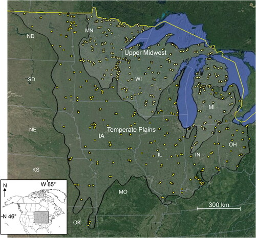
The purpose of this paper was to survey natural and anthropogenic variables of streams in the central US, specifically the Temperate Plains and Upper Midwest ecoregions (Herlihy et al. 2008; Omernik and Griffith 2014; Herlihy et al. 2020) (Figure 1). The former region is composed of ∼9,00,000 km² of tallgrass prairies and hardwood forest, with most habitats converted to pasture or row crops. The latter region composes ∼4,00,000 km² and remains mostly covered by either hardwood or coniferous forests. Previous stream classification studies within portions of the study area were of smaller scale (n ≤ 100 stream sites) and included only site-specific variables (Wang et al. 1998; Goldstein et al. 2002). The study area has some overlap with the eastern US of McManamay et al.’s (2018) study, mostly within IN, MI, and OH, but is otherwise an area that has not been studied using the geospatial datasets mentioned above.

Figure 1. The location of the Upper Midwest and Temperate Plains ecoregions showing the 819 stream sites assessed during this study. Substantial marker overlap occurs at this level of resolution. State abbreviations: IA: Iowa; IL: Illinois; IN: Indiana; KS: Kansas; MI: Michigan; MN: Minnesota; MO: Missouri; ND: North Dakota; NE: Nebraska; OH: Ohio; OK: Oklahoma; SD: South Dakota; WI: Wisconsin. Base maps: Google, National Institute of Statistics and Geography.

Further, potentially important variables, such as stream sinuosity, not addressed in McManamay et al. (2018) were included in this study. The specific objectives were to delineate overall patterns in physical conditions of stream sites in the two ecoregions, and relate these patterns to geographic and anthropogenic variables.

Materials and methods

Stream sites were chosen to maximize spatial distribution within the two ecoregions. To access the NHDPlus and StreamCat databases, the WATERSKMZ kml file (https://www.epa.gov/waterdata) was downloaded into Google Earth (GE). This interface allowed measuring streams along the transect using GE, while also having USEPA data about the same stream sites readily accessible. Once a general area was selected using GE, the nearest watershed was identified using NHDPlus Surfacewater Features. A line transect was placed across the streams of this watershed, at an angle that maximized stream intersections, and all of the sites intersected by the transect were selected for data acquisition.

Ten variables were used to classify the 819 selected stream sites (Table 1). Stream gradient (variable #1) was estimated using GE by determining the elevation at the site and the elevation of the stream 1–5 km above the site. The difference between the two values was divided by the measured length to calculate percent gradient. Stream sinuosity (2) was estimated by measuring a straight line in GE 1–5 km above the site to the site. Dividing the measured value of actual channel distance to this point by the value of the straight line calculated stream sinuosity. Mean summer stream temperature (3) for all years available (2008, 2009, 2013, 2014), base flow as a percentage of total stream flow (4), the percentage of organic matter in the surrounding soil (5), soil permeability (6), mean distance to bedrock (7), mean distance to water table (8), composite topographic index (CTI) (9), and total runoff value (10), all at the local (Hydrologic Unit Code-12) catchment scale, were determined using the StreamCat database.

Table 1. Site physical characteristic variables used in this study, with their sources and summary statistics.

No.	Name	Source	High	Low	Mean	SE
1.	Stream gradient	Rise/run over 1–5 km stream distance using GE	9.7	0.3	1.8	0.32
2.	Stream sinuosity	Channel/straight line distance using GE	4.7	1.0	1.6	0.02
3.	Summer stream temperature (°C)	https://watersgeo.epa.gov/watershedreport. . . . . . . . . .	26.2	14.3	19.6	0.09
4.	Base flow as percent of total flow	https://watersgeo.epa.gov/watershedreport. . . . . . . . . .	88.3%	8.8%	48.5%	0.68%
5.	Soil organic matter (% by weight)	https://watersgeo.epa.gov/watershedreport. . . . . . . . . .	59.1%	0.2%	4.9%	0.26%
6.	Soil permeability (cm/h)	https://watersgeo.epa.gov/watershedreport. . . . . . . . . .	33.0	0.3	11.4	0.34
7.	Depth to bedrock (cm)	https://watersgeo.epa.gov/watershedreport. . . . . . . . . .	152.4	64.8	147.2	0.52
8.	Distance to water table (cm)	https://watersgeo.epa.gov/watershedreport. . . . . . . . . .	182.9	5.6	113.3	1.54
9.	Composite topographic index	https://watersgeo.epa.gov/watershedreport. . . . . . . . . .	1566.9	310.1	575.2	4.79
10.	Runoff (mm/month)	https://watersgeo.epa.gov/watershedreport. . . . . . . . . .	494.0	5.0	276.8	3.94

Ten geographic and anthropogenic variables were used as predictors of site characteristics (Table 2). Intact habitat (variable #11) was estimated from StreamCat by summing all land area within a site’s local catchment not classified as row crop, developed, or pasture, and expressing the sum as a percentage of total land area as ‘percent intact habitat’. All determinations used the most recent (2011) land cover data set. The percentage of each catchment occupied by non-native plants (12), percentage of site stream flow impounded by dams (13), percentage of catchment area under impervious surface (14), total length of roads (15), and number of people living within the catchment (16) were determined from StreamCat. Latitude (17), longitude (18), and elevation (19) were determined for each site using GE. The total watershed area upstream of each site (20) was determined from the NHDPlus database.

Table 2. Geographic and anthropogenic predictor variables used during this study, with their sources and summary statistics.

No.	Variable	Source	High	Low	Mean	SE
11.	Percent intact habitat	https://watersgeo.epa.gov/watershedreport. . . . . . . . . .	100.0%	0.0%	51.9%	1.12%
12.	Percent exotic plants	https://watersgeo.epa.gov/watershedreport. . . . . . . . . .	100.0%	0.0%	41.3%	1.15%
13.	Relative storage volume	https://watersgeo.epa.gov/watershedreport. . . . . . . . . .	17360.0	0.0	116.3	35.09
14.	Percent impervious surface	https://watersgeo.epa.gov/watershedreport. . . . . . . . . .	43.6%	0.0%	1.8%	0.14%
15.	Road density (km/km^2)	https://watersgeo.epa.gov/watershedreport. . . . . . . . . .	17.3	0.0	1.9	0.05
16.	Number of people per km^2	https://watersgeo.epa.gov/watershedreport. . . . . . . . . .	922.6	0.2	31.8	3.18
17.	Latitude	Measured at site, confirmed in GE	49.3°	35.3°	43.9°	0.10°
18.	Longitude	Measured at site, confirmed in GE	−82.2°	−101.9°	−90.2°	0.15°
19.	Elevation (m)	Measured at site, confirmed in GE	556	105	281.8	3.14
20.	Watershed area (km^2)	https://watersgeo.epa.gov/watershedreport. . . . . . . . . .	277694.2	1.4	2791.8	598.0

To delineate regional differences in stream site physical characteristics, and to assess the relative importance of geographic and anthropogenic variables in predicting these differences, the 819 measured sites were ordinated with principal components analysis (PCA) using the default settings of PC-ORD v.7. The primary data matrix consisted of the 10 physical variables for each of the 819 stream sites. A secondary matrix of the 10 geographic and anthropogenic variables was then joint plotted with the determined ordination.

Based on the PCA results, value range maps of the classes of the most important variables were then produced in GE to show geographic and ecoregional trends. Class ranges were adapted from McManamay et al. (2018). 100% stacked column graphs were made of catchment-level intact habitat per variable class within each ecoregion to estimate differences in disturbance per stream type. Maps of percent intact habitat associated with each stream site were also produced. Intact habitat was measured on three scales: local catchment as used in the PCA analysis, the 100 m riparian mask on either side of each stream within the local catchment, and the entire land area upstream of each site. All intact habitat data were obtained from the StreamCat database.

Results

The PCA ordination produced three significant axes (Figure 2). Axis 1 (27.4% of variation explained, p = 0.001) generally delineated sites of the two ecoregions based on differences in stream temperature, base flow, and soil permeability. Axis 2 (19.7%, p = 0.001) corresponded to intraregional differences in gradient, distance to bedrock and water table, and CTI. Axis 3 (13.0%, p = 0.001) corresponded to intraregional differences in stream sinuosity. Three predictor variables: latitude (R² = 0.22), percentage of non-native plants (R² = 0.35), and percentage of intact catchment habitat (R² = 0.33) all corresponded to PCA Axis 1. No other predictor variable had R² > 0.1 with any axis (Table 3).

Figure 2. Two-dimensional principle components analysis ordination of 819 stream sites based on the 10 analyzed site characteristic variables. A third significant axis is not shown. Geographic and anthropogenic predictor variables (arrows) with R² >0.20 based on regressions with the primary ordination shown in joint plot. Variable numbers in Tables 1–2.

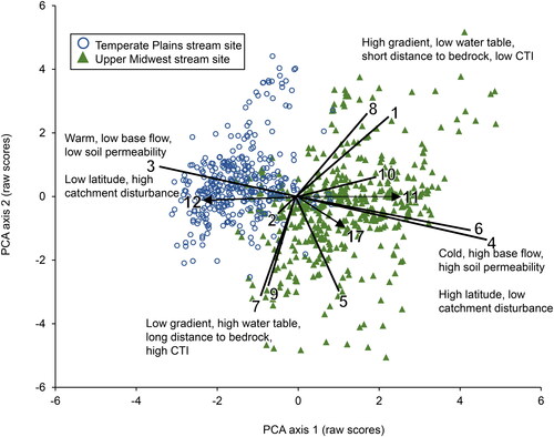
Table 3. Classification codes for the most important determined site characteristic variable for each of the three PCA axes, plus the commonly reported variables of watershed area and summer stream temperature.

Watershed area		Stream temperature		Gradient		Base flow		Sinuosity
Class	km^2	Class	(°C)	Class	%	Class	%	Class	Value
Headwater (HW)	0–10	Cold (Cd)	<19	Very low (VL)	<0.1	Very low (VL)	<20	VL	1.0–1.33
Creek (Cr)	10–100	Cold-cool (Cd-Cl)	19–21	Low (L)	0.1–0.5	Low (L)	20–40	L	1.33–1.66
Small river (SR)	100–500	Cool (Cl)	21–23	Moderate (M)	0.5–2	Medium (M)	40–60	M	1.66–2.0
Medium river (MR)	500–2500	Cool-warm (Cl-W)	23–25	Mod. high (MH)	2–4	High (H)	60–80	H	2.0–2.33
Mainstem (Ms)	2500–10,000	Warm (W)	>25	High (H)	4–10	Very high (VH)	>80	VH	>2.33
Large river (LR)	10,000–25,000
Great river (GR)	≥25,000

Site class ranges for watershed area, summer stream temperature, and gradient all taken from McManamay et al. (2018). Ranges for base flow and sinuosity estimated herein. 

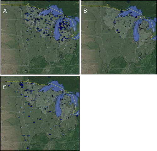
Due to the covariance among many variables of both PCA axes (Figure 2), value range maps were made only of the most important variable for each of the three axes: base flow, stream gradient, and stream sinuosity. High and very high base flow (>60%) was strongly associated with the Upper Midwest ecoregion, with most very high base flow stream sites found in northwestern Lower MI (Figure 3a). Stream gradient was generally low (<1%) throughout most of both ecoregions (Figure 3b). Nearly all moderately-high or high gradient streams (>2%) were found in northern MI or MN, and drained into either Lake Superior or the Saint Croix River. Most streams had low to medium sinuosity (1–2) (Figure 3c). Occasional highly sinuous streams were found throughout the study area, but most commonly in the western portion of the Temperate Plains.

Figure 3. Differences in percent of base of flow (A), stream gradient (B), and stream sinuosity (C) for the 819 streams analyzed in this study. Larger and darker markers represent higher values of each measure based on the ranges from Table 1. Base maps: Google, National Institute of Statistics and Geography.

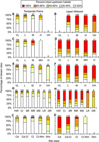
Streams with high or very high levels of intact upstream habitat (>60%) were found almost exclusively in the northeastern half of the Upper Midwest ecoregion (Figure 4a). Streams with high or very high intact local catchment habitat were found at a greater frequency throughout the study area (Figure 4b), as were streams with high or very high intact riparian habitat (Figure 4c). Taking the lowest value for each site from the three different scales (Figure 4d) demonstrated that nearly all streams of the Temperate Plains had low or very low intact habitat (<40%). The only very high intact habitats (>80%) were found in northeastern MN, northern WI, northern MI, and a small area of southern IN. Similar trends were found throughout the classes of the most important determined variables and also among size and temperature classes of streams (Figure 5).

Figure 4. The percentage of intact habitat upstream of each sampling site (A), in the local catchment of each sampling site (B), in the 100 m riparian zone of each sampling site (C), and reflecting all three aforementioned measures (D). Larger and darker markers represent greater intact habitat based on five categories: >80%, 60–80%, 40–60%, 20–40%, <20%. Base maps: Google, National Institute of Statistics and Geography.

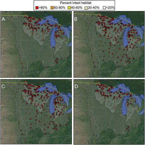
Figure 5. The percent of intact habitat (based on Figure 4d) of the two ecoregions based on the most important determined environmental variable for each significant PCA axis: percent base flow (A, B), stream gradient (C, D), and stream sinuosity (E, F), and also the commonly reported variables of watershed area (G, H) and stream temperature (I, J). Site classes and codes from Table 1. Sample size for each site class above its respective bar.

Discussion

Natural variation between streams of the two ecoregions was predominately that of differences in base flow and temperature. High base flow indicates high groundwater recharge and stable cold temperatures; such high values are known throughout the Upper Midwest, particularly northern Lower MI (Holtschlag 1997; Wolock 2003; Kelleher et al. 2012; Mayer 2012; McManamay et al 2018). Conversely, streams of the Temperate Plains have lower base flow and, thus, are more prone to flooding and warmer temperatures. Differences in stream temperature were also influenced by latitude and, thus, air temperature, as streams of the Upper Midwest were generally further north and in cooler ecosystems than those of the Temperate Plains.

Differences in stream sinuosity and stream gradient were less important on an ecoregion scale, since most streams of both ecoregions were of similarly low gradient and moderate sinuosity. Both variables, however, were locally important and produced outlier streams. The tributaries of Lake Superior, for example, are known for being high gradient and for containing unique assemblages of aquatic insects (Houghton 2015). Conversely, the very low gradient landscape of the western Temperate Plains produced the most sinuous streams (Tester 1995).

Similarly, variation in intact habitat was primarily on a landscape scale, and did not vary much between size of streams or other variable classes. Watershed-scale upstream habitat generally increased with latitude, with almost all undisturbed streams occurring in northern MI, MI, and WI. This pattern has been previously noted in MN (Houghton 2004), and renders difficult the separation of latitude and habitat effects. Intact habitat along the 100-m riparian mask of streams, while more abundant in northern MI, MI, and WI, was considerably more evenly distributed throughout the study area than was upstream habitat. Riparian buffers are frequently employed to mitigate the effects of agricultural input, and are frequently the only remaining forested habitat in agricultural watersheds (Craig et al. 2008; Burdon et al. 2020).

The primary exception to patterns of intact upstream habitat was a collection of streams in southern IN, protected by the Hoosier National Forest. Three streams had very high intact habitat based on the combination of riparian mask, catchment, and upstream habitat, and 5 had high intact habitat. These streams were ∼500 km from streams with similar levels of intact habitat. While most of these streams were tiny headwater springs protected by small watersheds, three streams: Little Blue River (latitude: 38.2909, longitude: −86.4890), Negro Creek (39.0033, −86.2625) and Patoka River (38.4422, −86.4873), had watershed areas of 14–128 km². While this study is not an exhaustive inventory of streams in this region, these results do suggest southern IN as an area of high conservation priority due to containing some of the least disturbed streams of the Temperate Plains.

One challenge to discerning the important variables affecting stream conditions is the presence of multiple co-varying temperature gradients. While percent of base flow had the strongest association with stream site temperature (Figure 2), latitude and percent upstream habitat exhibited similar patterns. All three factors clearly delineated the two ecoregions along a single axis. Base flow, latitude, and intact habitat are all known to influence stream temperature, due to cold groundwater upwelling, effects on air temperature, and differences in shading and sunlight penetration respectively (Ebersole et al. 2003; Allan 2004; Dugdale et al. 2020). Since all three variable gradients occur in the same direction, separating their relative importance will be difficult. Isaak et al. (2020) likewise found multiple temperature gradients when analyzing rivers of the western US.

While this study is not directly analogous to McManamay et al.’s (2018) study of the eastern US due to differences in variables measured and techniques used, some comparisons between results do emerge. In McManamay et al (2018), over half of the watersheds of the eastern US had ≥10% agricultural land cover, and 37% had ≥25%. If results are comparable, then the situation is worse in the northcentral US. Two-thirds of Upper Midwest watersheds had ≥10% agricultural land cover and 44% had ≥25%. In the Temperate Plains, >99% of watersheds had ≥10% agricultural land cover and 72% had ≥25%.

This study represents the first attempt to classify streams of the northcentral US using modern databases and methods. Such results are likely broadly applicable to ecosystems throughout temperate biomes, especially those with high levels of anthropogenic disturbance. It also indicates the importance of variables, like stream sinuosity, that are not readily available in USEPA databases and probably should be added to future iterations of them. Further research is needed throughout the US and elsewhere on the effects of these natural and anthropogenic stream variables, and stream classification systems in general, on biological assemblages such as fish or benthic macroinvertebrates.

Data accessibility statement

All data used in this study are available on the Open Science Framework site. https://osf.io/gqjt3/?view_only=d4f9d5bbcf184d28881cc26b2a572e6d

Acknowledgments

This is paper no. 24 of the G.H. Gordon BioStation Research Series. The comments of Angie Pytel improved an earlier version of the manuscript. Research and publication costs supported by the Hillsdale College biology department. Google Earth base maps displayed using permission guidelines (https://www.google.com/permissions/geoguidelines/attr-guide/).

Disclosure statement

No potential conflicts of interest were reported by the author(s).

Additional information

Funding

No external funding was received for this study.

Notes on contributors

David C. Houghton

David C. Houghton is a professor of biology at Hillsdale College and the director of the G.H. Gordon Biological Station. His research involves the biological diversity of aquatic organisms, particularly caddisflies, and the effects of natural and anthropogenic impacts on their assemblages.

References

- Allan JD. 2004. Landscapes and riverscapes: the influence of land use on stream ecosystems. Annu Rev Ecol Evol Syst. 35(1):257–284.
- Bastviken D, Tranvik LJ, Downing JA, Crill PM, Enrich-Prast A. 2011. Freshwater methane emissions offset the continental carbon sink. Science. 331(6013):50.
- Burdon FJ, Ramberg E, Sargac J, Forio ME, de Saeyer N, Mutinova PT, Moe TF, Pavelescu MO, Dinu V, Cazacu C, et al. 2020. Assessing the benefits of forested riparian zones: a qualitative index of riparian integrity is positively associated with ecological status in European streams. Water. 12(4):1178.
- Cole JJ, Caraco NF. 2001. Carbon in catchments: connecting terrestrial carbon losses with aquatic metabolism. Mar Freshwater Res. 52(1):101–110.
- Craig LS, Palmer MA, Richardson DC, Filoso S, Bernhardt ES, Bledsoe BP, Doyle MW, Groffman PM, Hassett BA, Kaushal SS, et al. 2008. Stream restoration strategies for reducing river nitrogen loads. Front Ecol Environ. 6(10):529–538.
- Downing JA, Cole JJ, Duarte CM, Middelburg JJ, Melack JM, Prairie YT, Kortelainen P, Strieg RG, McDowell WH, Tranvik LJ. 2012. Global abundance and size distribution of streams and rivers. IW. 2(4):229–236.
- Dugdale SJ, Hannah DM, Malcolm IA. 2020. An evaluation of different forest cover geospatial data for riparian shading and river temperature modelling. River Res Appl. 36(5):709–723.
- Ebersole JL, Liss WJ, Frissell CA. 2003. Cold water patches in warm streams: physicochemical characteristics and the influence of shading. J Am Water Resources Assoc. 39(2):355–368.
- Goldstein RM, Wang L, Thomas P, Simon P, Stewart PM. 2002. Development of a stream habitat index for the Northern Lakes and Forests ecoregion. North Am J Fish Manage. 22(2):452–464.
- Herlihy AT, Paulsen SG, Van Sickle J, Stoddard JL, Hawkins CP, Yuan LL. 2008. Striving for consistency in a national assessment: the challenges of applying a reference-condition approach at a continental scale. J North Am Benthol Soc. 27(4):860–877.
- Herlihy AT, Sifneos JC, Hughes RM, Peck DV, Mitchell RM. 2020. The relation of lotic fish and benthic macroinvertebrate condition indices to environmental factors across the conterminous USA. Ecol Appl. 112:105958.
- Hill RA, Weber MA, Leibowitz SG, Olsen AR, Thornbrugh DJ. 2016. The Stream Catchment (StreamCat) dataset: a database of watershed metrics for the conterminous United States. J Am Water Resour Assoc. 52(1):120–128.
- Holtschlag DJ. 1997. A generalized estimate of ground-water recharge rates in the Lower Peninsula of Michigan. U.S. Geological Survey Water-Supply Paper 2437, p. 37.
- Houghton DC. 2004. Biodiversity of Minnesota caddisflies (Insecta: Trichoptera): delineation and characterization of regions. Environ Monit Assess. 95(1-3):153–181.
- Houghton DC. 2015. Delineation and characterization of Michigan caddisfly biological diversity (Insecta: Trichoptera), and comparison with Minnesota. J Freshwater Ecol. 30(4):525–542.
- Isaak DJ, Luce CH, Horan DL, Chandler GL, Wollrab SP, Dubois WB, Nagel DE. 2020. Thermal regimes of perennial rivers and streams in the Western United States. J Am Water Resour Assoc. 56(5):842–867.
- Kelleher C, Wagener T, Gooseff M, McGlynn B, McGuire K, Marshall L. 2012. Investigating controls on the thermal sensitivity of Pennsylvania streams. Hydrol Process. 26(5):771–785.
- Mayer T. 2012. Controls of summer stream temperature in the Pacific Northwest. J Hydrol. 475:323–335.
- McManamay RA, DeRolph CR. 2019. A stream classification system for the conterminous United States. Sci Data. 6:190017
- McManamay RA, Troia MJ, DeRolph CR, Olivero Sheldon A, Barnett AR, Kao S-C, Anderson MG. 2018. A stream classification system to explore the physical habitat diversity and anthropogenic impacts in riverscapes of the eastern United States. PLoS ONE. 13(6):e0198439.
- Omernik JM, Griffith GE. 2014. Ecoregions of the conterminous United States: evolution of a hierarchical spatial framework. Environ Manage. 54(6):1249–1266.
- Raymond PA, Cole JJ. 2001. Gas exchange in rivers and estuaries: choosing a gas transfer velocity. Estuaries Coasts. 24(2):312–317.
- Tester JR. 1995. Minnesota’s natural heritage, an ecological perspective. Minneapolis (MN): University of Minnesota Press.
- Thorp JH, Thoms MC, Delong MD. 2006. The riverine ecosystem synthesis: bio-complexity in river networks across space and time. River Res Appl. 22(2):123–147.
- Wang L, Lyons J, Kanehl P. 1998. Development and evaluation of a habitat rating system for low-gradient Wisconsin Streams. North Am J Fish Manage. 18(4):775–785.
- Wolock DM. 2003. Estimated mean annual natural ground-water recharge estimates in the conterminous United States. U.S. Geological Survey Open-File Report 03-311. https://water.usgs.gov/lookup/getspatial?rech48grd.