Anthropogenic drivers of plant species coexistence in selected riparian systems, Kumawu district, Ashanti region (Ghana)

Abstract

Anthropogenic drivers have long been recognized as influencing species coexistence and the maintenance of biodiversity in riparian ecosystems among others. Despite their important role, riparian zones have been subjected to progressive alteration. This study aimed at evaluating how anthropogenic drivers influence plant species coexistence in riparian zones differing in scale of disturbance – intact zone (Amobia), slightly disturbed zone (Onwame), moderately disturbed zone (Ninian) and degraded zone (Pame), respectively, located in the Kumewu District of Ahanti Region (Ghana). Plots were randomly laid perpendicular to the anthropogenic gradients such as fire, grazing pressure, erosion, farming, animal trampling, bare ground and logging. Number of individuals was counted per plot and the percentage cover estimated per species. Species packing model was employed to quantify how competing species for resources coexisted, while Canonical correspondence analysis (CCA) was used to evaluate the effect of anthropogenic drivers on the variability of species assemblages. High number of species heterogeneity at Amobia riparian zone was a reflection of their tolerance to species coexistence than in the severely disturbed Pame riparian zone. However, species optimum and maximum probability of occurrence tend to be highest in Pame and lowest at Amobia riparian zone. This may be that widespread driver like fire, grazing pressure, farming and logging created conditions in gaps suitable for the recruitment of diverse species, with functional traits facilitating coexistence. These anthropogenic disturbances were responsible for 53.48% variability in species composition and coexistence. Thus, to enhance species coexistence, restoration of severely disturbed Pame, should be of priority concern by park managers.

Keywords:

• Species packing
• canonical correspondence analysis
• disturbance-related drivers
• riparian quality index
• protected areas
• species diversity

Introduction

The earth’s ecosystem is undergoing unprecedented rates of change, from a combination of anthropogenic environmental drivers of change (Brooker 2006; Díaz et al. 2019; Moullec et al. 2021). Anthropogenic drivers, which consist of the mechanisms limiting plant biomass by causing its destruction (Grime 1977; Chidumayo 2014; Ma et al. 2021), has long been recognized as influencing species coexistence and the maintenance of biodiversity (Connell 1978; Huston 1979). Plant–plant interactions are an important part of the mechanisms governing the response of plant species and communities to anthropogenic drivers of change (Brooker 2006). Anthropogenic drivers of change such as farming practices, fire, grazing pressure, logging, are diverse in nature and have been noted for their adverse impact on plant species coexistence in different ecosystems. The Millennium Ecosystem Assessment (MA) defines a driver as any natural or human-induced factor that directly (physical and biological) or indirectly causes a change in an ecosystem (Carpenter et al. 2006; Nelson et al. 2006). A direct driver influences ecosystem processes, while an indirect driver operates in a more diffused form by altering one or more direct drivers (Nelson et al. 2006).

In a potentially productive environment, the mechanism of disturbance can occur as: (1) a low intensity of disturbance that modifies the balance between competitive species, and (2) severe disturbance which selects species with phenology adapted to exploit temporarily favorable conditions destruction (Grime 1977). These drivers of change be it natural or anthropogenic or a combination, are acting to influence species composition or function of natural systems (Brooker 2006).

Biodiversity conservation along riparian corridors, in the face of increasing threat of anthropogenic drivers of change, have been recognized by many scientists and government as a policy priority (Secretariat of the Convention on Biological Diversity 2003; González et al. 2017). Thus, impact of anthropogenic drivers of change on species composition and communities, could have profound consequences on ecosystem services, supporting the livelihood of many rural dwellers. Giving these phenomena, there is justifiable reason to understand the underlying drivers of change that influences species coexistence and ultimately determine the ecological integrity and biodiversity of riparian ecosystems, especially among the riparian zones where this study is conducted (Amobia, Ninian, Onwame and Pame riparian zones, all in the Sekyere Kumawu and Afram plains District of Ghana’s Ashanti Region).

Riparian forests are one of the most valuable ecological elements of river systems. They maintain high levels of biological diversity and productivity and provide dynamic habitats for many different species (Bennett and Simon 2004). They also provide ecological and social benefits, ecosystem services, perform critical functions in both hydrological and biogeochemical cycles, protect water quality, and rich diversity of flora and fauna (Naiman and Decamps 1997; Knight and Bottorff 2020).

Riparian vegetation in Ghana, play a crucial role in rural livelihood support, in a form of herbal medicine extraction. Other services include a refugia for wildlife, especially in the wildlife sanctuary where this study was conducted. However, due to progressive alteration of the forest ecosystem in, the Sekyere Kumawu and Afram plains District mainly linked to bushfires, expansion of farming activities, grazing pressure, and animal trampling in the last decade, it has not been explicitly studied how and to what extent these anthropogenic disturbances affected species composition in riparian ecosystems including the four riparian systems considered in this study. Even at the National level, there is equally no study on how anthropogenic disturbances influence species composition and ultimately their coexistence. Thus, giving the importance of species coexistence in ecosystem functioning, it is vital to understand how plant species respond to varied anthropogenic disturbances and its overall effect on species composition and diversity of the four riparian ecosystems.

Amobia and Onwame are located in the protected area of Bomfobiri Wildlife Sanctuary, while Pame and Ninian riparian zones are found in the Bufuom forest reserve (production reserve) and unprotected area of Soboyo community, respectively, in the Sekyere Kumawu and Afram plains District of Ghana’s Ashanti Region. Onwame, Ninian and Pame riparian zones, constitute a continuum along the tributaries off the main Amobia riverine system and also serve as transboundary wildlife corridors between the protected and the unprotected areas.

The aim of this study was to understand how anthropogenic disturbances-related drivers influenced species composition and coexistence at differing scale of disturbance in the four riparian zones: intact zone (Amobia), slightly disturbed zone (Onwame), moderately disturbed zone (Ninian) and degraded zone (Pame). To achieve the aim of this study, we asked the following questions:(1). What is the level of plant species tolerance to disturbance-related drivers?(2) what are the implications of disturbance-related drivers on species optima, tolerance, and maximum probability of occurrence in each level of disturbance gradient?(3) what is the effect of disturbance-related drivers on species richness and diversity?(4) How were plant species partitioned into their niche space in terms of similar response to disturbance magnitude, among the four riparian zones?

We hypothesized in this research that: (1) increased magnitude of anthropogenic drivers of change would result in a lower level of species tolerance, (2) disturbance-related drivers will not bring about variations in species optima, tolerance and maximum probability, (3) plant assemblages will differ in their response to anthropogenic drivers and animal disturbance, since the magnitude (i.e. scope and severity) of driver impact in each riparian zone will likely vary. Secondly, response to anthropogenic drivers is species-specific, because different species in a community, will have different resistance and resilience to habitat perturbation (Grime 1979; Lawes et al. 2016).

Methods

Study area

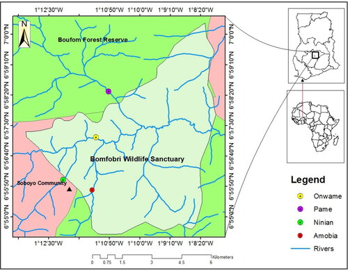
The study was conducted at Bomfobiri Wildlife Sanctuary (BWS – a strict protected area), Boufum Forest Reserve (BFR – a production reserve) and Soboyo community (unprotected area or off-reserve), all in the Kumawu District of Ashanti Region (Ghana). The focus areas were on the four riparian zones (i.e. Amobia, Onwame, Pame and Ninian riparian zones). Amobia and Onwame riparian zones are located in Bomfobiri Wildlife Sanctuary, Ninian and Pame riparian zones are in the Soboyo community and Boufum Forest Reserve, respectively. The study area lies between latitude 01°20′ N and 01°20′ N and longitudes 6°52’W and 7°32’W (Figure 1). The GPS coordinates of the four riparian zones where plant species were sampled are shown in Appendix 1 (Supplementary material). Bomfobiri Wildlife Sanctuary and Boufum Forest Reserve, hereinafter be known as BWS and BFR, and the four riparian zones also as Amobia riparian zone, Onwame riparian zone, Ninian riparian zone and Pame riparian zone. Bomfobiri Wildlife Sanctuary and Boufum forest reserve are surrounded by four major towns and about eight adjacent farming communities. The dominant vegetation types include riverine forest, savanna woodland and grassland Sekyere Kumawu District Assembly (SKDA)) (2014). The study area experiences double maxima rainfall pattern, beginning from March to July and the second starting from September to October (Mihaye 2013). Mean annual rainfall is around 1250 mm and 1740 mm (Mihaye 2013). Average annual temperature ranged between 32 °C in the dry season (November to March) and 25^°C during the wet season (April to October), with a relative humidity of 70%–80%. The geology of the area is typical of the Voltaian system, with the soil type comprising of shallow Leptosols on sandstone outcrops and forest Ochrosols (red, fine sandy loam) and savanna soils (Bomfobiri Wildlife Sanctuary Management Plan 1994–2004). Topography is characteristically mountainous, with flat plain at some section of the savannah zone, undulating hilly and sloppy grounds, and valleys mainly nearer to the water bodies. (Appendix 2, Supplementary material).

Figure 1. Map of Ghana, showing the three study areas (Bomfobiri Wildlife Sanctuary Source and Boufrom Forest Reserve – Protected areas and Soboyo community – unprotected area), in the Kumawu District. The four riparian zones are represented by the following colours in the legend: yellow – Onwame riprian zone (ORZ), violet – Pame riparian zone (PRZ), bright green – Ninian riparian zone (NRZ) and red – Amobia riparian zone.

Classification of the four riparian zones

Initial survey of the riparian zones revealed different disturbance-related driver levels among the four riparian zones. We subsequently used the Riparian Quality Index (RQI) method (Gonzalez del Tanago and Garcia de Jalon 2011) to classify the condition state of each of the four riparian zones, using the three-point criteria. The application of the RQI, which was habitat-specific, gave rise to the following classifications: Amobia (intactzone), Onwame (slightly disturbed zone), Ninian (moderately disturbed zone) and Pame (degraded zone). These classifications alongside differing disturbances are supported by Osborne and Kovacic (1993), who stated that for any lotic system, a continuum of environmental conditions can exist ranging from a 'natural or pre-impacted' state to a degraded 'impacted' state. The RQI method constitute a standardized survey method use to assess ecological status of riparian zones; an element of the river morphological conditions considered by the Water Framework Directive. Secondly, the method is applied to monitor, diagnose, restore and set conservation priorities to post-project evaluation (Gonzalez del Tanago and Garcia de Jalon 2011). The RQI index range between 1 and 15. For the purposes of this study, we classified the four riparian sites, using the first three criteria proposed by (Gonzalez del Tanago and Garcia de Jalon 2011), and which include: (1) Dimensions of land with riparian vegetation; (2) Longitudinal continuity, coverage and distribution pattern of vegetation along riparian corridor and (3) Composition and structure of riparian vegetation (see details in Table 1).

Table 1. Riparian quality index method (RQI) (Gonzalez del Tanago and Garcia de Jalon 2011), used to classify the four riparian zones according to their different habitat conditions, in Bomfobiri Wildlife Sanctuary and Boufum forest reserve and Soboyo community.

	RQI	Disturbance level	Criteria 1	Criteria 2	Criteria 3
Amobia riparian zone	13–15	Intact condition zone	Vegetation connecting with upland species and covers all land between channel and adjacent slopes)	Usually, different vegetation strata cover the entire length of the segment, showing a heterogeneous distribution pattern, linked to natural fluvial forms and flood dynamics, without alterations related to human actions).	Riparian corridor including a mix of species corresponding to the indigenous vegetation associations of the river segment, with different strata (canopy, understory, ground cover) often including shade and climbing plants. No exotic species.
Onwame riparian zone	10–12	Slightly disturbed zone	Average width of riparian corridor slightly restricted by human action	Riparian vegetation covers the entire stretch of the segment but, with slightly reduced coverage, being higher than 60 % of natural coverage, and includes several strata.	Riparian vegetation slightly altered by human actions, with the presence of some alien invasive.
Ninian riparian zone	7–9	moderately disturbed zone	areas where vegetation covers nearly half of the riparian zone being disturbed	1–3 m active channel width and about 10–30% exotic	ruderal species present
Pame riparian zone	1–6	Degraded zone	areas where 60% of the riparian corridor is reduced by human-led activities	vegetation appears in small patches of < 30% (mainly grasses/herbs and isolated woody species), with channel banks connected to agricultural fields	more than 60% of coverage of exotic species, ruderal or alien invasive, due to land use.

Application of the RQI classification was riparian habitat-specific.

Vegetation survey

We initially carried-out a ground validation survey to identify and mark-out the different plant community types ((refers to as dominant plant cover or vegetation type, in a designated geographical unit), identified on the topographic map of the study area, using Etrex Garmin global position survey (GPS). The dominant vegetation types include: riverine forest, savanna woodland and grassland (Sekyere Kumawu District Assembly (SKDA)) (2014), whereas the dominant species in the intact (Amobia) and slightly disturbed zone (Onwame) include: Pseudospondias microcarpa, Triclisia patens and Blighia welwitschii, while the moderate (Ninian) and severely (Pame) disturbed zones included: Aspilia Africana, Euphorbia heterophylla, Hypselodelphyspoggeana, Senna alata and Panicum maximum. The natural water regimes shaping the riparian vegetation riparian are permanent (i.e. Amobia and Onwame riparian zones) and seasonal (i.e. Ninian and Pame riparian zones) flow discharge. The seasonal flow regime (especially in the wet season – April–September), is largely due to loss of tree cover, huge amount of sediment deposits on the river bed, flash flood and high evapotranspiration.

Stratified random sampling method (e.g. Stohlgren et al. 1997; Grabherr et al. 2003) was used to assess plant species in each of the four riparian zones (refers to as dominant plant cover or plant community, in a designated geographical unit). A total of 30 plots of 10 × 10 m (100 m²) dimensions for trees/shrubs and 0.5 × 2 m (1 m²) for grasses/herbs, were randomly laid in the different plant community types, bringing the total to 120 (30 plots per each riparian zone). The bigger plot sizes were 96, while the smaller plots were 24 in number. Random sampling technique was used in order to ensure that individuals of the sampled species population were adequately represented in all the four riparian zones and to maximize species heterogeneity. Plant species parameters such as `cover abundance, species presence/absence and diameter at breast height (DBH) were collected in 30 plots each of the four riparian zones (= 120 plots in total), from August to December, 2018. Sampling was done twice, covering the five-month period, and only new species that were detected in the repeated sampling were registered. Plots were laid perpendicular to the disturbance-related drivers (described in the next sub-section), in order to determine how plant species responded to these drivers of change such as fire, grazing pressure, erosion, farming, animal trampling, bare ground and logging. The Daubenmire cover-abundance classes were used to estimate ground cover of each species in each plot (Daubenmire 1959). Trees of height ≥ 1.4 m with a diameter at breast height (DBH) of ≥ 4 cm were sampled. Plants were identified up to species level, with the aid of plant identification keys provided by Okezie and Agyakwa (1998) and Arbonnier (2004).

Assessment of disturbance-related drivers

Disturbance-related drivers of change such as fire, grazing pressure, erosion, farming, animal trampling, bare ground and logging, in the protected (Bomfobiri Wildlife Sanctuary and Boufoum forest reserve) and unprotected areas (Soboyo community), were identified and measured in plots where the plant species were sampled. Here, a driver is defined according to the Millennium Ecosystem Assessment (MA), as is any natural or human-induced factor that directly (physical and biological) or indirectly causes a change in an ecosystem (Neuhauser and Pacala 1999; Carpenter et al. 2006). A direct driver influences ecosystem processes, while an indirect driver operates in a more diffused form by altering one or more direct drivers (Nelson et al. 2006). To determine how the plant community responded to the different threats, disturbance-related drivers were quantified using the Salafsky et al. (2003) and Battisti et al. (2009) methods. The scores for scope of the drivers were assigned as follows: 4: the driver is found throughout (50%) the sample plot; 3: the driver is spread in 15–50% of the sample plot; 2: the driver is scattered (5–15%); and 1: the driver is much localized (< 5%) (Battisti et al. 2009). Thus, a score of 1 = the lowest impact and 4 = the highest impact) was used to assess scope, severity and magnitude of every threat. For ‘scope’, we referred to the percentage ratio of the study site affected by a specific driver within the last 5 years (Battisti et al. 2009). To verify whether all the identified drivers in this study (i.e. fire, grazing pressure, erosion, farming, animal trampling and logging) persisted in the last 5 years and beyond, a one-on-one field interview with Park Managers of the two protected areas (BWS and BFR) and farmers from the Soboyo community (unprotected area) was undertaken.

For ‘‘severity’’ we referred to the degree to which a driver has impacted on the integrity of the plant community across the four riparian sites (both protected/unprotected areas) within the last 5 years. A score of 4 was assigned if the direct driver led to serious damage or loss of species; 3 if induced a serious damage; 2 if induced a moderate damage; 1, little or no damage. Finally, we calculated the ‘‘magnitude’’ which is the combination (sum) of the value score for scope and severity assigned to a specific driver per plot and ranked from highest to lowest (Salafsky et al. (2003). These drivers of change may be added either together, multiplied, or averaged, since in arithmetic calculations (addition, multiplication or average) relative order does not change (Salafsky et al. 2003).

Statistical analysis

(1). What is the level of plant species tolerance to disturbance-related drivers?

Canonical correspondence analysis (CCA) was performed to evaluate the relationship between species assemblages and the distribution of associated disturbance-related drivers or gradients (ter Braak 1987a, 1987b; Kent and Coker 1992), measured in each of the 120 plots following the Salafsky et al. (2003) and Battisti et al. (2009). CCA is a direct gradient analysis extension of correspondence analysis (CA) (ter Braak 1986; Palmer et al. 2010, 2018) that incorporate correlation and regression between floristic data and environmental factors within the analysis (ter Braak and Prentice 1988; Kent and Coker 1992) and extract the most important environmental environmental factors and floristic data sets (ter Braak and Verdonschot 1995). We chose CCA over other multivariate models (e.g. RDA) because species abundances are rescaled to a Q matrix, and their weights are derived from the species abundance matrix and applied to the explanatory variables (ter Braak and Verdonschot 1995, Legendre and Legendre 1998; Wagner 2004). For analyses of relative abundances, we initially transformed the abundances of floristic data at each site using log (X + 1). Due to the non-normal nature of the data set following Shapiro-Wilk (W = 0.614, p < 0.05, Shapiro – Wilk test), we applied Kruskal–Wallis H test (a rank-based nonparametric test approach) to determine whether overall species abundance, richness and diversity significantly differed among the four riparian zones. We also used Kruskal–Wallis test to determine whether disturbance-related drivers substantially differed across the four riparian zones, while Dunn’s post hoc test (Dunn 1961) was used to determine which riparian zones contributed significantly to the variability. All analyses were performed using PAST ver. 3.06 software package (Hammer et al. 2001).

(2). What are the implications of disturbance-related drivers on species optima, tolerance, and maximum probability of occurrence in each level of disturbance gradient?

Analysis of species coexistence (species packing) and competition for resource utilization within a niche space

Species packing model (Gaussian curve or lognormal distribution curve) (Gauch Jr and Chase 1974) was employed to determine how competing species for resources coexisted in their niche space (n-dimensional environmental space) and niche overlaps, following observed disturbance-related drivers or driver magnitude on species abundance, at plot level/riparian zone. This is an ecological model based on the idea that during evolution species evolve to occupy maximally separated niches with respect to a limiting resource (MacArthur 1969).

Because species generally show unimodal relationships with environmental variables (Whittaker 1967), we fitted the Gaussian curve equation in the ecological dataset using the three parameters – maximum, optimum and tolerance, as shown below: $${\mathit{Ey}}_{\mathit{ik}}=\mathrm{ }{c}_k\text{e exp}.-\frac{1}{2}({x_i-u_k)}^2/{{\mathit{t}}_{\mathit{k}}}^2$$

(1) (Gauch Jr and Chase 1974).

Where y_ik = the abundance of species k at site i (i = 1…… n; k = 1…….m), Ey_ik = is the expected abundance, $x_i$ = the value of disturbance-related driversx at site i, $c_k\mathrm{ }=$ the maximum of the curve for species k, $u_k=$ the optimum (the value of x with highest probability of occurrence of species k) of species k, i.e. the value of x for which the maximum is attained, ${t_k}^2$ the tolerance (a measure of ecological amplitude) of species, which is a measure of curve breadth or ecological amplitude. This problem involves the maximum likelihood (ML) estimation of site scores (xk) and the species’ optima (uk), tolerances (tk) and maxima (ak), usually by an alternating sequence of Gaussian (logit) regressions and calibrations (Gauch Jr and Chase 1974; Kooijman 1977; Kooijman and Hengeveld 1979; Goodall and Johnson 1982; Ihm and van Groenewoud 1984). The ordination axes were constructed using the disturbance-related drivers in order to optimize the fit of the species data to a particular (linear or unimodal) statistical model of how species abundance varies along gradients ter Braak 1985; ter Braak 1987a, 1987b).

(3). What is the effect of disturbance-related drivers on species richness and diversity?

Analysis of species richness and diversity

Chao-1 species estimate model, was employed to compare estimated species richness among the four sites, using the non-asymptotic approach (Chao and Chiu 2014). The assumption of Chao-1 model is that one or more samples have been taken by collection, from one or more assemblages for some specified group or groups of organisms (Gotelli and Colwell 2001).

Hill numbers (MacArthur 1960; Hill 1973; Jost 2006, 2007; Chao et al. 2014) was applied to quantify and compare current species diversity status among the four riparian zones. We used this model because Hill numbers are a mathematically unified family of diversity indices (differing among themselves only by an exponent q) that incorporate relative abundance and species richness and overcome many of shortcomings of other diversity indices (Chao et al. 2014; Hill 1973). Hill numbers or effective number of species model equation is provided below: (4) $${}^{q}D={\left(\sum _{i=1}^S{p}_i^q\right)}^{1/(1-q)}$$(4) in which S is the number of species in the assemblage, and the i_th species has relative abundance p_i, i = 1, 2, …, S. The parameter q determines the sensitivity of the measure to the relative frequencies.

(4). How were plant species partitioned into their niche space in terms of similar response to disturbance magnitude, among the four riparian zones?

Results

Plant species composition and their tolerance to disturbance-related drivers

A total of 1,589 individuals belonging to 48 families and 141 species were sampled from the four riparian zones (Table 2). Majority of the species (14.2%) were from the Fabaceae, followed by Poaceae (8.5% species) (See Appendix 1, Supplementary material). The moderately disturbed zone registered the highest mean number of individuals (n = 440, 9.58 ± 1.4 per plot), while the least was recorded at the slightly disturbed zone (n = 374, 4.6 ± 0.4 per plot) (Table 2). Canonical component analysis (CCA) diagram segregated species in each of the riparian zones (at plot level) according to their response level to disturbance-related drivers (Figure 2a, b). Majority of plots that were strongly associated with disturbance-related drivers, with higher magnitude scores (i.e. scope and severity of a disturbance-related driver) for bushfire (n = 4), logging (n = 4), grazing (n = 3), erosion (n = 3.5) and animal trampling (n = 3), were largely from Pame and Ninian riparian zones, while the least disturbance was recorded in Amobia (n = 1) riparian zone (Figure 2a, Table 3). Plots clustered around the centre of the CCA ordination diagram, exhibited weak association with nearly all the disturbance-related drivers. (Figure 2a).

Figure 2. a & b: Principal component analysis (PCA) diagram, showing variability in species response to seven disturbance-related drivers in the 120 plots, across the four riparian zones. Plot codes represent the following: ARZ = Amobia riparian zones; ORZ = Onwame riparian zones; NRZ = Ninian riparian zones and PRZ = Pame riparian zone. The black dots represent plant species (e.g. Kyllinga bulbosa = Kbulb, Mariscus longibracteatus = Mlong, Setaria sphacelate = Sspha andPaspalum distichum = Pdist), while the arrows represent the disturbance-related drivers plotted pointing in the direction of maximum change of explanatory variables of the different sample plots. Axis I = 31.74% and Axes II = 21.74% jointly explained 53.48% influence of disturbance-related drivers on the habitat condition and species coexistence.

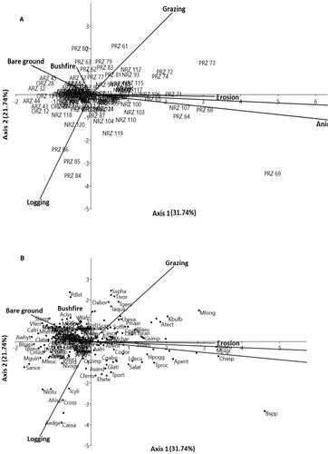
Figure 3. Gaussian curve or lognormal distribution curve showing how competing species at plot level coexist in their niche space (n-dimensional environmental space) and niche overlaps, along environmental gradient. Notice that severely disturbed Ninian and Pame riparian zones, recorded high species abundance at plot level, whereas less disturbed zone like Amobia, had less abundant species. The x-axis represents disturbance-related drivers in sample plot/riparian zone, calculated as the ‘driver magnitude’ (i.e. a sum of the value score for scope and severity assigned to a specific driver per plot and ranked from highest to lowest – Salafsky et al. 2003; Battisti et al. 2009 ).The alphabets denote the following: u = optimum, t = tolerance and m = maximum.

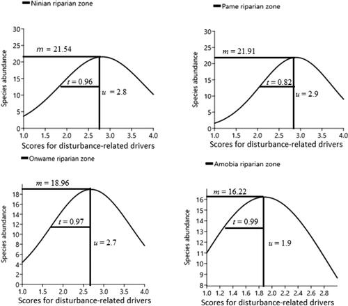
Table 2. Mean number of plants sampled in each of the 120 plots, across the four riparian zones.

Site	No. of Individuals	Mean ± SE	Variance (s^2)
	374
Amobia riparian zone (Intact zone)		4.6 ± 0.4	12.81
Onwame riparian zone (slightly disturbed zone)	365	5.35 ± 0.5	18.31
Ninian riparian zone (moderately disturbed zone)	440	9.58 ± 1.4	101.98
Pame riparian zone (degraded zone)	410	10.25 ± 1.1	48.24

Amobia and Onwame are located in Bomfobiri Wildlife Sanctuary (a strict protected area). Ninian and Pame are located in the Soboyo community (unprotected area or off-reserve) and Boufum Forest Reserve (a production reserve), respectively. (n = 1,589).

Table 3 Summary of the average scores for seven disturbance-related drivers assessed in each of the 120 plots among the four riparian zones.

Anthropogenic drivers	Onwame riparian zone scores	No. of plots	Amobia riparian zone scores	No. of plots	Pame riparian zone scores	No. of plots	Ninian riparian zone scores	No. of Plots
Bushfire	4	1	2	3	4	5	3	6
Grazing	1	10	1	7	4	8	2	5
Erosion	1	3	1	4	4	3	3	2
Farming	1	4	1	1	4	6	3	2
Animal trampling	2	6	1	12	3	3	3	5
Bare ground	1	1	1	2	4	1	2	4
Logging	3	5	2	1	4	4	3	6

The average scores (magnitude) is a combination of the scope and four severity scores of each disturbance-related driver.

Species that were found to be tolerant to marked disturbance-related drivers among plots in Pame and Ninian riparian zones included: Panicum maximum (Pmaxi, n = 85) and kyllinga bulbosa (Kbulb, n = 21), from the upper right of the CCA diagram (Figure 2b; Appendix 1, Supplementary material). The two grass species were the most abundant and widely distributed in the two zones (located in the off-reserve or unprotected area and the production reserve). The two zones were characterized by severe grazing pressure (r = 0.48, P > 0.05), farming (r = 0.84, P < 0.0001), animal trampling (r = 0.84, P < 0.0001) and erosion (r = 0.64, P < 0.001) (Tables 3, 4). Fewer trees, lianas and herb species that equally showed tolerance to similar severe disturbance-related drivers, in Ninian and Pame riparian zones, (i.e. lower right of the diagram), were Aspiliaafricana (Aafri, n = 58), Euphorbia heterophylla (Ehete, n = 29), Hypselodelphyspoggeana (Hpogg, n = 19), Senna alata (Salat, n = 19), Trianthemaportulacastrum (Tport, n = 15) and Tridax procumbens (Tproc, n = 12) (Figure 2b). These species were influenced by bare ground (r = −0.59, P < 0.05), bushfire (r = 0.82, 0.0001), and farming (r = −0.50, P < 0.05) along axis II and bushfire (r = −0.42, P < 0.05) on axis I (Tables 3, 4). Seven species constituted singletons (rarer species) (e.g. Bussea occidentalis, Celtis zenkarii, Ficus exasperata, Khaya grandifolia and Wakangaafricana) and represented 0.4% of total individuals sampled. These appeared to have been affected by disturbance-related drivers mostly in Pame and Ninian riparian zones. The first two axes accounted for 53.48% (Axis I = 31.74 and II = 21.74) cumulative percentage variance for the site-disturbance-related driver biplot (Figure 2, Table 5). These disturbance-related drivers substantially differed across the four riparian zones (Hc = 31.19, p < 0.05, Kruskal-Wallis test), with Amobia and Ninian, Onwame and Pame riparian zones contributing significantly to variability in disturbance-related drivers (p < 0.05, Dunn’s post hoc test). Intercorrelation among the seven disturbance-related drivers revealed a significant correlation between farming and animal trampling (r_s = 0.62, P < 0.01). This phenomenon was observed especially where crop raiding by elephants and other ungulates was widespread among farmlands close to the riparian zones. Correlation between grazing and animal trampling (r_s= 0.42, P < 0.01) was equally observed in Pame and Onwame (Figure 2a, Table 5).

Table 4. Summary of CCA axis lengths, showing the levels of correlation between four riparian zonesand seven disturbance-related driver gradients and percentage variance in species assemblages in 120 plots.

CCA Axes	I	II	III
Eigenvalue	2.22	1.52	1.06
Total % variance	31.74	21.74	15.27
Cum. Total % variance explained	31.74	53.48	68.76
Bushfire	−0.42	0.82***	0.33
Grazing	0.48*	0.22	−0.18
Erosion	0.64**	0.15	0.61**
Farming	0.84***	0.05	−0.17
Animal trampling	0.84***	0.08	−0.37
Bare ground	0.29	−0.59**	0.59**
Logging	−0.27	0.65**	0.09

Asterisks (*) = disturbance-related drivers thatwere significant. A correlation above/below ±0.70 is significant at ***p = 0.001; ±0.60 at **p = 0.01and > 0.44 at *p = 0.05.

Eigenvalues were significant for axes I (P < 0.011) & II (P < 0.013, Monte-Carlo P)

Table 5. Spearman Rank Intercorrelations between the environmental variables.

	Bushfire	Grazing	Erosion	Farming	Animal trampling	Bare ground	Logging
Bushfire		0.24	0.028*	0.34	0.3441	0.001*	0.0003*
Grazing	0.11		0.0061*	0.036*	0.0002*	0.8	0.44
Erosion	0.22	0.26		0.0017*	0.0709	0.06	0.44
Farming	0.095	0.22	0.31		0.0001*	0.72	0.06
Animal trampling	−0.095	0.42	0.18	0.68		0.87	0.37
Bare ground	−0.33	−0.03	0.19	0.037	−0.017		0.0073*
Logging	0.37	−0.08	−0.076	−0.19	−0.087	−0.26

NB: Values above the black diagonal line represent the level of significant, whereas those below represent their respective correlation statistics (R2).

Species packing and competitive equilibrium of the plant species across the four riparian zones

Species from the low disturbed riparian zones (i.e. Amobia (intact zone) and Onwame (slightly disturbed) riparian zones, appeared to exhibit a higher ecological amplitude or tolerance (T_amp = 0.99 and T_amp = 0.97, respectively) compared to Ninian (T_amp = 0.96) and Pame (T_amp = 0.82) riparian zones, that were severely disturbed (Figure 3). However, species optimum (which is a measure of the environmental condition under which maximum number species is attained), was found to be high in Pame (u = 2.9), Ninian (u = 2.8) and Onwame (u = 2.7) than in Amobia (u = 1.9) riparian zones. Under maximum probability of species occurrence, only some limited portion of potential species niche space (related to estimated gradients and many other characteristics that were not considered) has been estimated, and was found to be equally higher in Pame (c = 21.91), Ninian (c = 21.5) and then in Amobia (c = 16.22) riparian zones (Figure 3). The species maximum recorded in each of the four riparian zones were determinant of the optimum (u) anthropogenic drivers calculated under the Gaussian curve.

Influence of disturbance-related drivers on species richness and diversity

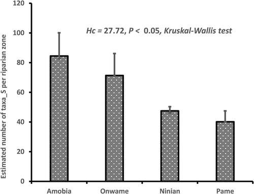
Effect of disturbance-related drivers contributed markedly in species richness among the four zones (Hc = 27.72, P < 0.05, Kruskal–Wallis test). Observation from individual riparian zones revealed that the severe impact of disturbance-related drivers (i.e. grazing, farming and logging) reflected in the species poor status of Pame (S = 40.13 Chao-1 estimate) and Ninian (S = 47.5 Chao-1 estimate) riparian zones (Figure 4). In contrast, the intact zone of Amobia riparian zone, where impact of disturbance-related driver was less, was the most species rich (S = 84.44, Chao-1 estimate). Plant functional group types in this riparian zone were largely trees (n = 24), lianas (n = 13) and shrub (n = 7) species.

Figure 4. Comparison of estimated species richness among the four riparian zones.

Species diversity equally differed among the four riparian zones (Hc = 7.615, P = 0.05, Kruskal– Wallis test), and were ranked from highest to lowest diversity index, along alpha (α) scale values of 0.04 to 3.96 (Figure 5, Table 6). Dunn’s post hoc test revealed that Pame and Amobia (P < 0.03) and Ninian and Amobia (P < 0.03) riparian zones substantially contributed to variations in species diversity. But from individual riparian zones, we found Pame riparian zone (severely degraded zone) to be the most species diverse of α scale = 0.04, Hill numbers (^qD) = 2.99, to α scale = 3.96, ^qD = 2.86), in spite of being the most species poor (Figure 5, Table 6). The high diversity in Pame riparian zone was largely a reflection of the species evenness distribution as shown in the shallow diversity curve (Figure 5). Grass (7.8%) and herb (5.7%) species, constituted the major plant functional groupings in Pame riparian zone; an evidence of its current transformed state into a typical savannah vegetation, linked to widespread disturbance-related driver impact. The moderately disturbed zone of Ninian riparian system was the least diverse (α-scale = 0.04, ^qD = 2.94 to α-scale = 3.96, ^qD = 2.57), as shown its steepest curve (bottom curve in turquoise colour). This was a reflection in its lowest evenness distribution of species and number of individuals among the sampled plots (Figure 5, Table 6).

Figure 5. Hill numbers showing diversity profiles among the four riparian systems, in the protected and unprotected areas. Variability in the shape of the curves is indicative of species evenness distribution patterns in each of the four riparian systems. Thus, shallow curve reflects high diversity of a site, while steep curve indicates less diversity.

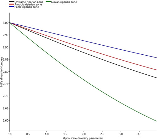
Table 6. Summary of Hill numbers (at α = 0, 1 and 2), Hill species diversity and Shannon_Evenness, across the four riparian zones in protected and unprotected areas, at Kumawu District of Ghana.

Alpha values	Onwame	Amobia	Pame	Ninian
0(Number of sp.)	70	81	39	44
1(exp[Shannon])	53.32	63.58	30.53	30.04
2(Inv.[Gini_Simpson)	42.28	50.83	26.79	21.53
Shannon_Evenness	0.76	0.78	0.79	0.67
Hill’s numbers	2.77	2.81	2.86	2.59

The order q, which is mathematically unified family of diversity indices differing among themselves only by an exponent q, and which indicates their tendency to include or ignore the relatively rarer species (Hill 1973). Thus, q = 0, represent number of species in the sample (richness index), q = 1, exponential of the Shannon-Weiner index and q = 2, reciprocal of the Simpson’s index (i.e. equivalent number of species).

Discussion

Plant species composition and their tolerance to disturbance-related drivers

Environmental disturbances play a key role in shaping plant community structure (Hughes 2010). We found in this study that the identified drivers such as bushfires, farming activities, grazing pressures, logging and animal trampling, contributed in the reduction of species heterogeneity and species coexistence particularly in Pame riparian zone. Impacts of fires, farming activities and grazing pressure, have reportedly altered soil nutrients, reduction in plant gene pool and introduction of alien invasive species, among riparian wetlands in biogeographical zone (Oksanen 1983), similar to where this study was conducted. Despite the basis for the Intermediate disturbance hypothesis, which states that diversity of competing species is maximized at intermediate frequencies (Bongers et al. 2009), our findings was inconsistent with the principle behind IDH, since species diversity enhances species coexistence, we expected species coexistence to rather be higher at slightly degraded Onwame riparian zone and moderately degraded Ninian riparian zone. But in contrast, species coexistence along disturbance gradient was observed to decrease symmetrically as disturbance intensity increases from the intact Amobia riparian zone through to the degraded Pame riparian zone. Our findings appear to be supported by Fox (2013), and who argued on the basis that empirical studies on IDH rarely find the predicted humped diversity-disturbance relationship and the three theoretical mechanisms claimed to produce this relationship are logically invalid. The three theoretical mechanisms stated as follows, posit that species richness (and diversity) at the local scale peaks at (1) intermediate values of disturbance frequency, (2) intermediate times after a disturbance, and (3) at intermediate spatial extents of disturbance (Grime 1973; Horn 1975; Connell, 1978). Huston (2014) also argued that diversity of competing species at maximum frequencies can also depend on the diversity-productivity relationship (intermediate productivity hypothesis – IPH) rather than IDH.

Many researches have shown that increases in soil resource availability and grazing pressure are the two fundamental drivers of environmental change for plant communities (Adler et al. 2001; Laliberté et al. 2013). However, even though soil nutrient parameters were not factored in our study, research have shown that bushfire (which was the most predominant driver of change observed in all the four riparian zones) has a strong implication on soil nutrient availability (Wilbur and Christensen 1983; Schmalzer and Hinkle 1992; Heinl et al. 2007). Bushfires observed in these riparian zones were mainly caused by group hunters who deliberately set fire to drive animals out so they can kill them, control burning as a conservation strategy against wildfire during the dry season, by Park managers and annual burning to improve the quality of forage for livestock and land preparation for farming activities, by indigenous farmers. Even though bushfire has been used as conservation strategy in many plant communities to open up canopy cover and allow recruitment and germination of propagules, the direct effect bushfire have on soil resource availability reduces productive resources available to support plant growth. This tends to displace off low competing species, by allowing species of highly competitive ability (such as invasive species) to take a tract on the riparian zones. The consequence of this driver impact, may lead to high intraspecific competition in the long term and eventually reduce species coexistence.

The severe grazing pressure in Pame riparian zone as compared to the remaining three riparian zones, was due to the fact that water availability all year round, made livestock and other wild ungulates to preferably graze at the riparian zone than other the terrestrial zones. This tends to exert much pressure on the riparian vegetation. Such unrestricted livestock grazing causes disturbances that have a number of damaging effects, namely; grazing and trampling on vegetation, inhibiting regeneration, soil compaction and creation of pathways and transporting of plant seeds (or seeds of invasive species) in their fur and droppings (Nsor et al. 2019). Animal trampling was observed as a direct replica effect of grazing pressure and farming activities. As more livestock graze on a particular riparian zone, their trampling effect on the soil becomes more intense, causing soil compaction and consequently inhibiting plant growth. Also, crop-raiding caused by Buffalos (from Bomfobiri Wildlife Sanctuary – BWS) on the farmlands along the riparian zones, increased trampling effect of animals. This tends to the bareness of the land and consequently, susceptible to erosion.

Species packing and competitive equilibrium of the plant species across the four riparian zones

This study explored how anthropogenic drivers affect species coexistence under disturbance gradient due to spatial storage effects. We observed that, across a wide range of disturbance-related drivers, Amobia riparian zone (intact zone) and Onwame riparian zone (slightly disturbed zones) that were characterized by low disturbance gradients, exhibited high level of tolerance range. Our observation corroborated with the statement by MacArthur (1970) that, by the properties of approximations, a very large number of competing species can coexist and tolerate each other if the environmental production is constant. These subtle properties of periodic fluctuations could have important consequences on ecological amplitudes, as a result of environmental function imposing a particular distribution of environmental states on ecological stability (Kremer and Klausmeier 2017). The statement by Kremer and Klausmeier (2017) probably explain why a consequent high tolerance or ecological amplitude was observed in Amobia (classified as intact zone), Onwame (Slightly disturbed), and Ninian (moderately disturbed) riparian zones, in spite of the high number of species recorded from these riparian zones. Thus, the number of species competing for resources may not necessarily be influence severely their tolerance range to impacts of drivers and limited resources within a niche space. Buttel et al. (2002) shared similar view and stated that species may compete for a common resource, without being limited simply by its availability, because species differ in the way they utilize the resource (Buttel et al. 2002). But May and MacArthur (1972) on the contrary argued that, comparatively high environmental disturbance and low resource production, are the chief limitations to species coexistence. It has also been long recognized that, in communities with variety of systems such as riparian zones, even in the presence or absence of stochastic influences (MacArthur and Levins 1967; Turelli 1986), there is no limit to the number of competing species that can coexist (Tilman 1994).

The high maximum species entry and a consequent high species optimum but low species tolerance observed in Pame riparian zone (i.e. the severely degraded zone), may be due to the fact that severe occurrence of disturbance-related drivers such as logging, farming and bushfire, led to the removal of plant species, and simultaneously created gaps up for new species to colonize the system. Asynchronous gap formation, either due to exogenous heterogeneity or natural deaths of individuals, can create opportunities for colonization and an almost infinite subdivision of successional gradients (Linda et al. 2002). Also, in utilization of a resource spectrum, MacArthur (1970) noted that ‘where the utilizations fall slightly below the production, a new species can enter if the addition of one pair (or propagule) will make the total utilization even closer to the available production’. While sufficient environmental resources (rather than simply the metabolic requirements for survival) are essential for organisms to channel energy into growth and reproduction (Hunter 2002), we suggest that the probability of colonization and survival of new species would not only depend on resource availability, but also the species optimum – which is a measure of the environmental condition under which maximum number species is attained.

Influence of disturbance-related drivers on species richness and diversity

In spite the low species richness in the severely degraded Pame riparian zone, it was the most diverse across the four riparian zones. This may be due to the fact that reduction in ground cover linked to impacts of disturbance-related drivers, created an even distribution pattern among species, which tended to reduce stress and competition among species in a niche space. Such scenarios tend to promote equitable resource utilization and regeneration of species. The second reason could be due to the presence of infrequent species (e.g. Bussea occidentalis, Celtis zenkarii, Ficus exasperata, Khaya grandifolia and Wakangaafricana) – described as species with a low probability of encounter, restricted range size or habitat specificity (Rabinowitz 1981; Kondratyeva et al. 2019), that thrived from severe disturbances. Ricotta and Avena (2002) and Dazzo et al. (2013) indicated that shallower declining curves (an indicator of high diversity) are more spatially even in species abundance distribution than steeper slopes (less diverse).

Apart from the spatially even distribution of species, which is as an indicator of high diversity, the lower proportion of rarer species may have contributed to the high diversity in the severely degraded Pame riparian zone. This is because, in measure of ecological diversity (which is an indicator of ecological health or integrity), the mean contribution of each species in ecological functioning is very critical. The concept of species rarity and originality have been widely used in diversity assessment (Patil and Taillie 1982; Kondratyeva et al. 2019). Prior to the application of the concept of species rarity and originality (Patil and Taillie 1982; Kondratyeva et al. 2019), Rabinowitz (1981) made a foremost proposition of a typology of rare plant species characteristics used as indicators of diversity of a site, to include: local population size (high or low), geographic range (large or small) and habitat specificity (wide or narrow). While Gaston (1997) also listed abundance, threat aspects (extinction risk) and value aspects (‘how special species are’), as biological aspects of species rarity used to determine diversity of an ecosystem.

The low diversity recorded in Amobia and Onwame (intact and slightly disturbed zones, respectively), despite being species richness was probably due to the uneven distribution of the high abundance of individuals per plot. This phenomenon tended to increase competition for space and resource utilization among species in their niches, and consequently leads to plant stress and low survival. Secondly, the relatively low disturbance impact in these riparian zones could have accounted for the low diversity. While low or no disturbance may increase the presence of indigenous gene pool, an optimal degree of disturbance to open the closed canopy, may facilitate the recruitment of new species and their evenness distribution pattern. Al though, this management intervention may achieve the desired objective of increasing species diversity, severe disturbance has the potential of reducing overall diversity through the destruction of sensitive late-succession species (Bongers et al. 2009).

Conclusion

Generally, spatial heterogeneity played a functional role in species coexistence, but only under low environmental disturbance gradient as overserved in Amobia, Onwame and Ninian riparian zones. Thus, a high disturbance gradient under spatial heterogeneous environment, as occurred in Pame riparian zone, could disrupt species coexistence, and this can have a direct effect on species diversity. Spatial heterogeneity promotes species diversity, and high species diversity itself can also increase spatial heterogeneity.

Environmental drivers such as bushfires, farming, logging and grazing pressure, negatively impacted on the plant communities, and are presumably going to reduce species fitness up to the point to limit their tolerance, and impair their coexistence, if current trends of anthropogenic drivers are not halted. Even though under increase in environmental pressure, species coexistence could be maintained by changes in species interactions (through increased role of facilitation and complex multi-species interactions reinforcement), this becomes possible if species are able to buffer the pressure through their functional variability, in order to compensate for the limited number of species making up the community. Since species coexistence arises from a number of factors, such as competition among species (either conspecific or heterospecific) towards a common available resource, spatial heterogeneity and environmental heterogeneity, a decrease in human-led driver impacts especially in Pame riparian zone (degraded zone), can substantially shape observed patterns and enhance species ecological optima, through increase in species tolerance among a large number of diverse species.

Author’s contributions

CAN, JNM and VRB conceived the ideas and designed methodology; JNM, VKK, VA, VRB and PAA carried-out field data collection, identification of species and data entry in excel sheet; CAN and JNM analyzed the data and led the writing of the manuscript. All authors contributed critically to the drafts and gave final approval for publication.

Declaration

The field data collection complied with the current laws of the country in which they were performed.

Acknowledgments

We express our appreciation the management of Bomfobiri Wildlife Sanctuary, for their assistance in locating the sites for this study and support during field sampling. Finally, our heartfelt gratitude to Mr. Dabo, for his guidance during species identification.

Disclosure statement

The authors declare no conflict of interest exists.

Data availability statement

The code and data used in the analysis of this study, will be publicly accessible at Dryad Digital Repository (https://datadryad.org/).

Additional information

Funding

This study was self-funded by the authors.

Notes on contributors

Collins Ayine Nsor

Dr. Collins Ayine Nsor is an Aquatic Ecologist and currently a senior lecturer at the Department of Forest Resources Technology, Kwame Nkrumah University of Science and Technology. Nsor, has undertaking extensive research in freshwater ecosystems spanning from 2010 till date. His research is focused on the flora wetlands in Savanna and Forest zones of Ghana.

John Nkrumah Mensah

John Nkrumah Mensah (a former undergrad student in the Department of Forest Resources Technology, Kwame Nkrumah University of Science and Technology), is currently a PhD. Student at the University of Nebraska - Lincoln, School of Biological Science (USA). John previously worked on riparian systems in Ghana’s Ashanti Region. His current research interest is in the area of Plant population ecology.

Victor Rex Barnes

Dr. Victor Rex Barnes is an Ecologist, specializing in fire ecology and climate change. He is a senior lecturer at the Department of Agroforestry, Kwame Nkrumah University of Science and Technology. Rex has over 10 years of research experience in the area of ecosystem sciences and climate change mgt in natural and planted ecosystems.

Peter Kwesi Akomatey

Peter Kwesi Akomatey (a former undergrad student in the Department of Forest Resources Technology, Kwame Nkrumah University of Science and Technology), is currently a taxonomy specialist at RMSE Division of Forestry Commission of Ghana.

References

- Adler P, Raff D, Lauenroth WK. 2001. The effect of grazing on the spatial heterogeneity of vegetation. Oecologia. 128(4):465–479.
- Arbonnier M. 2004. Trees, shrubs and liannes of West Africandry zones. CTA-The Netherlands, Wageningen: CIRAD, MagrafMnhn.
- Battisti C, Luiselli L, Teofili C. 2009. Quantifying threats in a Mediterranean wetland: are there any changes in their evaluation during a training course? Biodivers Conserv. 18(11):3053–3060.
- Bennett SJ, Simon A. 2004. Riparian vegetation and fluvial geomorphology. Vol. 8. American Geophysical Union. Ecology 72(5):1678–1684.
- Bomfobiri Wildlife Sanctuary Management Plan. 1994–2004. Wildlife Division of the Forestry Commission (Ghana).
- Bongers F, Poorter L, Hawthorne WD, Sheil D. 2009. The intermediate disturbance hypothesis applies to tropical forests, but disturbance contributes little to tree diversity. Ecol Lett. 12(8):798–805. 01329.x
- Brooker RW. 2006. Plant-plant interactions and environmental change. New Phytol. 171(2):271–284. 01752.x.
- Buttel LA, Durrett R, Levin SA. 2002. Competition and species packing in patchy environments. Theor Popul Biol. 61(3):265–276.
- Carpenter SR, Bennett EM, Peterson GD. 2006. Scenarios for ecosystem services. Ecol Soc. 11(1):29. http://www.ecologyandsociety.org/vol11/iss1/art29/.
- Chao A, Chiu CH. 2014. Species richness: estimation and comparison. Wiley StatsRef: Statistics Reference Online, 1–26.
- Chao A, Gotelli NJ, Hsieh TC, Sander EL, Ma KH, Colwell RK, Ellison AM. 2014. Rarefaction and extrapolation with Hill numbers: a framework for sampling and estimation in species diversity studies. Ecol Monogr. 84(1):45–67.
- Chidumayo EN. 2014. Estimating tree biomass and changes in root biomass following clear-cutting of Brachystegia-Julbernardia (miombo) woodland in central Zambia. Environ Conserv. 41(1):54–63.
- Connell JH. 1978. Diversity in tropical rain forests and coral reefs. Science. 199(4335):1302–1310.
- Connell JH. 1978. Diversity in Tropical Rain Forests and Coral Reefs: High diversity of trees and corals is maintained only in a nonequilibrium state. Science. 199(4335):1302–1310.
- Daubenmire RF. 1959. Canopy coverage method of vegetation analysis. Northwest Sci. 33:39–64.
- Dazzo FB, Klemmer KJ, Chandler R, Yanni YG. 2013. In situ ecophysiology of microbial biofilm communities analyzed by CMEIAS computer-assisted microscopy at single-cell resolution. Diversity. 5(3):426–460.
- Díaz S, Settele J, Brondízio ES, Ngo HT, Agard J, Arneth A, Balvanera P, Brauman KA, Butchart SH, Chan KM, et al. 2019. Pervasive human-driven decline of life on Earth points to the need for transformative change. Science. 366 (6417). https://doi.org/https://doi.org/10.1126/science.aax3100
- Dunn O. 1961. Multiple comparisons among means. J Amer Statistical Assoc. 56(238):52–64.
- Fox JW. 2013. The intermediate disturbance hypothesis should be abandoned. Trends Ecol Evol. 28(2):86–92.
- Gaston KJ. 1997. What is rarity?. In: Kunin WE., Gaston KJ, editors. The biology of rarity. London: Chapman & Hall, p. 30–47.
- Gauch Jr HG, Chase GB. 1974. Fitting the Gaussian curve to ecological data. Ecol. 55(6):1377–1381.
- Gonzalez del Tanago M, Garcia de Jalon D. 2011. Riparian Quality Index (RQI): a methodology for characterising and assessing the environmental conditions of riparian zones. J. Limnetica. 30(2):0235–0254.
- González E, Felipe-Lucia MR, Bourgeois B, Boz B, Nilsson C, Palmer G, Sher AA. 2017. Integrative conservation of riparian zones. Biol Conserv. 211:20–29.
- Goodall DW, Johnson RW. 1982. Non-linear ordination in several dimensions. Vegetatio. 48(3):197–208.
- Gotelli NJ, Colwell RK. 2001. Quantifying biodiversity: procedures and pitfalls in the measurement and comparison of species richness. Ecol Letts. 4(4):379–391.
- Grabherr G, Reiter K, Willner W. 2003. Towards objectivity in vegetation classification: the example of the Austrian forests. Plant Ecol. 169(1):21–34.
- Grime J. 1973. Competitive exclusion in herbaceous vegetation. Nature. 242:344–347.
- Grime JP. 1977. Evidence for the existence of three primary strategies in plants and its relevance to ecological and evolutionary theory. Am Nat. 111(982):1169–1194.
- Grime JP. 1979. Plant strategies and vegetation processes. Chichester: Wiley.
- Hammer Ø, Harper DAT, Ryan PD. 2001. PAST: paleontological statistics software package for education and data analysis. Paleo Electr. 4(1):9.
- Heinl M, Sliva J, Murray-Hudson M, et al. 2007. Postfire succession on savanna habitats in the Okavango Delta wetland, Botswana. Afr J Ecol. 6:350–358.
- Hill MO. 1973. Diversity and evenness: a unifying notation and its consequences. Ecology. 54(2):427– 432..
- Horn HS. 1975. Forest succession. Sci Am. 232(5):90–98. https://doi.org/http://dx.doi.org/10.1038/scientificamerican0575-90.
- Hughes A. 2010. Disturbance and diversity: an ecological chicken and egg problem. Nat Edu Knowl. 3(10):48.
- Hunter MJ. 2002. Fundamentals of conservation biology. 2nd ed. Cambridge (MA): Blackwell Science.
- Huston MA. 1979. General hypothesis of species diversity. Am Nat. 113(1):81–101.
- Huston MA. 2014. Disturbance, productivity, and species diversity: empiricism vs. logic in ecological theory. Ecology. 95(9):2382–2396.
- Ihm P, van Groenewoud H. 1984. Correspondence analyses and Gaussian ordination. In: Chambers JM, Gordesch J, Klas A, Lebart, L, Sint PP, editors. Compstat lectures., Vienna, Wurzburg: Physica-Verlag; p. 5–60.
- Jost L. 2006. Entropy and diversity. Oikos. 113(2):363–375.
- Jost L. 2007. Partitioning diversity into independent alpha and beta components. Ecology. 88(10):2427–2439.
- Kent M, Coker P. 1992. Vegetation description and analysis. A practical approach. Chichester, UK: Wiley.
- Knight A, Bottorff R. 2020. The importance of riparian vegetation to stream ecosystems. In: Warner R, Hendrix K, editors. California riparian systems. Berkeley: University of California Press; p. 2159–2167. https://doi.org/https://doi.org/10.1525/9780520322431-025
- Kondratyeva A, Grandcolas P, Pavoine S. 2019. Reconciling the concepts and measures of diversity, rarity and originality in ecology and evolution. Biol Rev Camb Philos Soc. 94(4):1317–1337.
- Kooijman SALM, Hengeveld R. 1979. The description of a non-linear relationship between some carabid beetles and environmental factors. In: Patil GP, Rosenzweig ML, editors. Contemporary quantitative ecology and related ecometrics. Fairland (MD): The International Co-operative Publishing House; p. 635–647.
- Kooijman SALM. 1977. Inference about dispersal patterns [dissertation]. University of Leiden, Leiden, The Netherlands.
- Kremer CT, Klausmeier CA. 2017. Species packing in eco-evolutionary models of seasonally fluctuating environments. Ecol Lett. 20(9):1158–1168.
- Laliberté E, Lambers H, Norton DA, Tylianakis JM, Huston MA. 2013. A long-term experimental test of the dynamic equilibrium model of species diversity. Oecologia. 171(2):439–448.
- Lawes MJ, Keith, DA, Bradstock RA. 2016. Advances in understanding the influence of fire on the ecology and evolution of plants: a tribute to Peter J. Clarke. Plant Ecol. 217:597–605.
- Legendre P, Legendre L. 1998. Numerical ecology. 2nd English ed. Amsterdam, The Netherlands: Elsevier.
- Linda AB, Richard D, Simon AL. 2002. Competition and species packing in patchy environments. Theor Popul Biol. 61:265–276. http://www.idealibrary.com.
- Ma H, Mo L, Crowther TW, Maynard DS, van den Hoogen J, Stocker BD, Terrer C, Zohner CM. 2021. The global distribution and environmental drivers of aboveground versus belowground plant biomass. Nat Ecol Evol. 5(8):1110–1122..
- MacArthur R. 1960. On the relative abundance of species. Am Nat. 94(874):25–36.
- MacArthur R. 1969. Species packing, and what competition minimizes. Proc Natl Acad Sci USA. 64(4):1369–1371.
- MacArthur R. 1970. Species packing and competitive equilibria form any species. TheorPoptn Biol. 1(1):1–11.
- MacArthur R, Levins R. 1967. The limiting similarity, convergence, and divergence of coexisting species. Am Nat. 101(921):377–385.
- May RM, MacArthur RH. 1972. Niche overlap as a function of environmental variability. Proc Natl Acad Sci USA. 69(5):1109–1113.
- Mihaye J. 2013. Small-scale mining operations and their effects in the East Akim Municipal Assembly [Doctoral dissertation]. University of Ghana.
- Moullec F, Asselot R, Auch D, Blöcker AM, Börner G, Färber L, Ofelio C, Petzold J, Santelia ME, Schwermer H, et al. 2021. Identifying and addressing the anthropogenic drivers of global change in the North Sea: a systematic map protocol. Environ Evid. 10(1):19..
- Naiman RJ, Decamps H. 1997. The ecology of interfaces: riparian zones. Annl Rev Ecol Syst. 28(1):621–658.
- Nelson GC, Bennett E, Berhe AA, Cassman K. 2006. Anthropogenic drivers of ecosystem change: an overview. Ecol Soc. 11(2):29. http://www.ecologyandsociety.org/vol11/iss2/art29.
- Neuhauser C, Pacala SW. 1999. An explicitly spatial version of the Lotka-Volterra model with interspecific competition. Ann Appl Probab. 9:1226–1259.
- Nsor CA, Antobre OO, Mohammed AS, Mensah F. 2019. Modelling the effect of environmental disturbance on community structure and diversity of wetland vegetation in Northern Region of Ghana. Aquat Ecol. 53(1):119– 136. https://doi.org/https://doi.org/10.1007/s10452-019-09677-5.
- Okezie IA, Agyakwa CW, editors. 1998. A handbook of West African weeds. Ibadan: International Institute of Tropical Agriculture (IITA) Nigeria, African Book Builders Ltd, p. 57.
- Oksanen J. 1983. Ordination of boreal heath-like vegetation with principal component analysis, correspondence analysis and multidimensional scaling. Vegetatio. 52(3):181–189.
- Osborne LL, Kovacic DA. 1993. Riparian vegetated buffer strips in water‐quality restoration and stream management. Freshwater Biol. 29(2):243–258.
- Palmer MA, Menninger HL, Bernhardt, E. 2010. River restoration, habitat heterogeneity and biodiversity: a failure of theory or practice?. Freshwater Bio. 55(S1):205–222.
- Palmer HD , Denham AJ, Ooi MK. 2018. Fire severity drives variation in post-fire recruitment and residual seed bank size of Acacia species. Plant Ecol. 219(5):527–537.
- Patil GP, Taillie C. 1982. Diversity as a concept and its measurement. J Am Stat Assoc. 77(379):548–561.
- Rabinowitz D. 1981. Seven forms of rarity. In: Synge H, editors. The biological aspects of rare plant conservation. Chichester: Wiley, p. 205–217.
- Ricotta C, Avena GC. 2002. On the information-theoretical meaning of Hill’s parametric evenness. Acta Biotheor. 50(1):63–71.
- Salafsky N, Salzer D, Ervin J, et al. 2003. Conventions for defining, naming, measuring, combining, and mapping threats in conservation. An initial proposal for a standard system. Draft version.
- Schmalzer PA, Hinkle CR. 1992. Soil dynamics following fire in Juncus and Spartina marshes. Wetlands. 12(1):8–21.
- Secretariat of the Convention on Biological Diversity. 2003. CBD Technical Series no. 10: Interlinkages between biological diversity and climate change. Advice on the integration of biodiversity considerations into the implementation of the United Nations Framework Convention on Climate Change and its Kyoto protocol. Montreal, Canada: Secretariat of the Convention on Biological Diversity.
- Sekyere Kumawu District Assembly (SKDA). 2014. District annual report, Republic of Ghana.
- Stohlgren TJ, Coughenour MB, Chong GW, Binkley D, Kalkhan MA, Schell LD, Buckley DJ, Berry JK. 1997. Landscape analysis of plant diversity. Landscape Ecol. 12(3):155–170.
- ter Braak CJF. 1985. Correspondence analysis of incidence and abundance data: properties in terms of a unimodal response model. Biometrics. 41(4):859–873.
- ter Braak CJF. 1986. Canonical correspondence analysis: a new eigenvector technique for multivariate direct gradient analysis. Ecology. 67(5):1167–1179.
- ter Braak CJF. 1987a. Ordination. In: Jongman RHG, ter Braak CJF, Van Tongren OFR, editors. Data analysis in community and landscape ecology. Waginingen: PUDOC; p. 91–173.
- ter Braak CJF. 1987b. The analysis of vegetation-environment relationships by canonical correspondence analysis. Vegetatio. 69(1–3):69–77.
- ter Braak CJF, Prentice IC. 1988. A theory of gradient analysis. Adv Ecol Res. 18:271–317.
- ter Braak CJF, Verdonschot PFM. 1995. Canonical correspondence analysis and related multivariate methods in aquatic ecology. Aquat Sci. 57(3):255–289.
- Tilman D. 1994. Competition and biodiversity in spatially structured habitats. Ecology. 75(1):2–16.
- Turelli M. 1986. Stochastic community theory: a partially guided tour. In Hallam TH, Levin SA, editors. Mathematical ecology: an introduction. Berlin: Springer-Verlag; p. 321–339.
- Wagner HH. 2004. Direct multi-scale ordination with canonical correspondence analysis. Ecology. 85(2):342–351..
- Whittaker RH. 1967. Gradient analysis of vegetation. Biol Rev Camb Philos Soc. 42(2):207–264.
- Wilbur RB, Christensen NL. 1983. Effects of fire on nutrient availability in a North Carolina coastal plain pocosin. Am Midld Nat. 110(1):54–61.