Hyporheic exchange due to in-stream geomorphic structures

Abstract

In-stream structures, such as channel spanning logs and weirs, can enhance hyporheic exchange in streams. Hyporheic exchange is important for stream ecosystem function, and restoring this function is a goal of many stream restoration projects. However, studies on the connection between in-stream structure size, hydrogeologic setting, and hyporheic exchange remain inadequately characterized. In this study, we combined flume experiments and numerical simulations to systematically evaluate how in-stream structure and its hydrogeologic setting impacted the hyporheic vertical exchange flux, Q, the solute penetration depth, D_p, and the solute flux, QS, in the hyporheic zone. The results showed that stream water downwells into the riverbed upstream of the weir and upwells downstream. Exchange rates were greatest near the weir and decay with distance upstream and downstream. Model results indicated Q, D_p and QS had a positive exponential relationship with the weir height, h, the flow velocity, u, and the sediment intrinsic permeability, k. While model results indicated that u was the most important factor determining Q, D_p and QS, followed by h, while only h reached a certain value, the hyporheic exchange would increase with the height and vice versa. Hyporheic exchange generally was sensitive to changes in k, only the magnitude of k varied from 10⁻⁸–10⁻¹⁰m². This finding suggests that a rethinking of the currently applied restoration techniques is required to better consider in-stream structure size, hydrological conditions and natural substratum dynamics in river restoration.

Keywords:

• In-stream structures
• hyporheic exchange
• stream restoration
• hyporheic vertical exchange flux
• solute penetration depth
• solute flux

1. Introduction

The hyporheic zone (HZ) is broadly defined as a ‘saturated transition zone between the surface water and groundwater beneath and adjacent to streams’ (Krause et al. 2009), and particularly is the zone where stream-borne substances are carried with the water into the subsurface, reside there for some time, and then return to the stream (Winter et al. 1998; Harvey and Wagner 2000; Packman and Bencala 2000). The exchange of water between a stream and its HZ (hyporheic exchange) has been demonstrated to have a substantial impact on stream ecological function, such as controlling the temperature pattern (Swanson and Cardenas 2010; Norman and Cardenas 2014), affecting the fate and transport characteristics of different solutes within the streambed (Packman et al. 2000; Ren and Packman 2004), altering the residence time of the solutes (Lautz et al. 2006), and enhancing nutrient cycling (Newbold et al. 1982; Tockner et al. 1999) with consequent benefits to stream ecosystem metabolism (Triska et al. 1989). Hence, hyporheic exchange has a significant effect on the stream ecological function (Boulton et al. 1998; Harvey and Gooseff 2015) and a substantial impact on the water quality of fluvial ecosystems (Findlay 1995; Hancock et al. 2005; Lewandowski et al. 2019).

Given the importance of the HZ, river restoration engineers and scientists have called for investigations into the influence of river restoration projects on hyporheic exchange (Hancock 2002; Boulton 2007; Boulton et al. 2010; Hester and Gooseff 2010). In-stream geomorphic structures (IGSs), such as rock cross vanes (Rosgen 2001; Buchanan et al. 2012; Daniluk et al. 2013; Gordon et al. 2013), channel spanning logs (Sawyer et al. 2011; Sawyer and Cardenas 2012), and steps (Chin et al. 2009; Endreny et al. 2011a) are commonly installed in stream restoration projects in natural and restored streams (Hester and Gooseff 2013). Knowledge of these in-stream structures driving hyporheic exchange is essential for understanding the solute transport characteristics within the streambed. These in-stream structures mainly affect hydraulic head gradients along the sediment-water interface (SWI), which drive hyporheic flow circulation of different lateral extents and penetration depths (Jiang et al. 2020).

In recent years, numerous field and laboratory studies have shown that in-stream structures have a significant effect on hyporheic exchange. The flume studies of Sawyer et al. (2011) developed equations for bed pressure profiles and hyporheic exchange rates in the vicinity of a channel-spanning log that can be used to evaluate the impact of large woody debris removal or reintroduction on hyporheic mixing. Smidt et al. (2015) used a time-lapsed electrical resistivity (ER) tomography to compare a stream restoration structure (cross-vane) and a natural feature (riffle) induced hyporheic exchange. The analysis indicated that restoration structures may be capable of creating sufficient exchange flux and timescales of transport to achieve the same ecological functions as natural features. Azinheira et al. (2014) showed that neither in-stream structures nor inset floodplains had sufficient percent flow and residence times simultaneously to have a substantial impact on dissolved contaminants flowing downstream. Menichino and Hester (2014) modeled weir-induced heat transport during summer. The results indicated that the thermal effect of the weir-induced exchange was therefore spatial expansion of subsurface diel variability, which affects benthic habitat and chemical reactions. Hester et al. (2009) concluded that weir-type structures will induce ecologically significant surface and subsurface thermal heterogeneity in many stream settings, but that weir-induced hyporheic heat advection will have ecologically significant thermal effects on surface water only in coarse streambeds. All of these studies on the effect of hyporheic restoration practices could be generalized in the following three aspects: (1) transforming bed pressure profiles, (2) creating sufficient exchange flux and residence timescales, and (3) varying the thermal regimes on enhancing the hyporheic exchange.

Similar to the aforementioned studies, other investigations have focused on improving the exchange flux through different structure designs, hydraulic conductivity and hydrogeologic setting. Hester and Doyle (2008) combined the models and a field study to systematically evaluate the impact of fundamental characteristics of the structure and its hydrogeologic setting on induced exchange. Model results indicated that structure size, background groundwater discharge rate, and sediment hydraulic conductivity are the most important factors determining the magnitude of induced hyporheic exchange, followed by geomorphic structure type, depth to bedrock, and channel slope. The study of Ward et al. (2011) through analyzing the designed structure length, structure height, and hydraulic conductivity, they concluded that the hyporheic flux could be potentially changed by hyporheic restoration structures. The numerical modelling research of Liu and Chui (2020) showed that the optimal height of the weir can be obtained by considering the nitrogen removal in the HZ.

Generalized, quantitative descriptions for hyporheic responses to in-stream structures and other hydrogeologic factors do not currently exist but would be useful for assessing changes in hyporheic exchange due to in-stream restoration projects. However, there is still a lack of simplified methods that can be widely used for preliminarily evaluating the suitability of hyporheic exchange of a natural and engineered stream and the design of in-stream geomorphic structures.

To fill this gap, this study provided a process-based understanding of how the in-stream structure affects hyporheic exchange in stream. This involved determining the relationships between the magnitude of in-stream structure induced hyporheic exchange and the fundamental characteristics of both the in-stream structure themselves (size) and of other settings (e.g. sediment intrinsic permeability, flow velocity). The weir for the specific case of a submerged, channel-spanning structure beneath the streambed is selected as the representative of in-stream structure since it is regarded as the most effective in improving the hyporheic flux (Hester and Doyle 2008). First, we conducted laboratory flume experiments to elucidate detailed descriptions of hyporheic exchange and solute transport in the underlying sediment due to a weir. Then, a sensitivity analysis was conducted to fully quantify the relationships between the size of in-stream structure, sediment intrinsic permeability, flow velocity and hyporheic exchange. Widely accepted and well tested two-dimensional models were chosen to model surface and groundwater response to sensitivity analysis perturbations using a simplified hypothetical stream setting to clearly separate the effects of various driving factors. Here we quantified and evaluated the HZ performance influenced by a weir using several indicators (e.g. hyporheic vertical exchange flux, Q, solute penetration depth, D_p, and solute flux, QS). Overall, this study will enhance our understanding and facilitate future studies regarding the evaluation of the in-stream structures induced HZ performance, which can be important for the stream ecosystem and benefit the restoration of the stream and the HZ.

2. Methods

2.1. Laboratory experiments

2.1.1. Flume setup

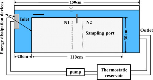
A custom-built recirculating flume tank consisting of a 150 cm long, 10 cm wide, and 50 cm deep rectangular channel (Figure 1) was used in the experiments. Tank walls were constructed from 1-cm-thick acrylic. One side of the tank had a 100 × 10 array of ports drilled into the acrylic at 3-cm spacing filled with plastic valve core, which allowed sampling of the water column and sediment pore water with a long hypodermic needle. The flume surface water temperature was controlled by a heating/cooling system attached to an additional water recirculation side loop. Water from the side loop mixes with the main recirculating loop. Surface water flow was then controlled by a valve and measured with an electromagnetic flow meter. Flow velocities of the flume was 0.04 m·s⁻¹. Damping devices at the upstream end of the flume minimized waves in order to obtain a smooth inflow into the study section. At the downstream end of the channel, a water-pervious, perforated Perspex sheet covered by a fine mesh was used to hold the sediment in place.

Figure 1. Schematic diagram of the custom built flume and other parts of the experimental apparatus. Light gray and blue areas represent sections filled with sand and water, respectively. The dark gray rectangle on the sand bed is a weir set up in the experiment. Sampling port locations, shown schematically.

2.1.2. Bed sand properties and preparation

A natural river sand from the Yangtze River was used. The sand was sieved to remove all fractions above 0.5 mm and washed repeatedly to remove fractions below 0.25 mm. The D₅₀ of the sand mix was 0.35 mm, yielding a sediment permeability of approximately 10⁻⁹ m². We conducted a set of experiments, where the objective of the experiments was to test the impact of the in-stream weir on the hyporheic exchange response. The total depth of the sediment column was 30 cm. To represent a channel spanning weir, a 15 cm tall channel-spanning weir was placed at the channel center and was cut to flume width and mounted 10 cm below the bed. The sediment grains beneath the weir were near the threshold for mobilization, and several grains moved by creep, but no significant scour topography formed.

2.1.3. Experimental conditions and measurements

The experiments also aimed to examine the solute transport processes in the streambed with a weir to quantify the solute penetration depth. In this study, we chose NaCl for the convenience of its measurement through electrical conductivity (EC). The relationship between concentration and EC of the NaCl solute at low concentrations is linear. At the beginning of the experiments, a measured quantity of the NaCl solution was added to the reservoir after the flume had run for 20 min (allowing the surface water flow to reach the steady state). To quickly achieve a uniform concentration (2.0 g·L⁻¹ for all the trails) in the surface water, the solute was added over the period of time it took for water to circulate around the system. To monitor the solute transport processes in the streambed, pore water samples were taken over time from the sampling ports. A 100-µL syringe with a fine needle was used to take samples through the plastic valve cores in the flume walls. A volume of 100-µL of pore water was extracted for each sample. The relatively small sampling volume was unlikely to significantly affect the flow field in the vicinity of the sampling port (Elliott 1990). The time interval of the pore water sampling was 30 min at the beginning of the experiment to capture the relatively rapid concentration change as the solute was transferred into the bed. As the experiment continued, the concentration change became gradual after the passage of the local solute front. The sampling time interval was increased to hours towards to the end of the experiment. The water sample was diluted with 5 ml of deionized water to allow sufficient volume for the subsequent EC measurement (using Mettler Toledo S230 manufactured by Switzerland).

2.2. Numerical simulations

A one-way sequential coupling method was used to simulate the stream water flow, and pore water flow and solute transport in the streambed. First, the stream water flow was simulated and the associated pressure distribution at the SWI was inferred. Then, the pore water flow in the bed, driven by the interfacial pressure variations was simulated. Finally, solute transport was simulated based on the pore water flow field. This method largely follows that of Cardenas (2006).

2.2.1. Mathematical model and boundary conditions for overlying water

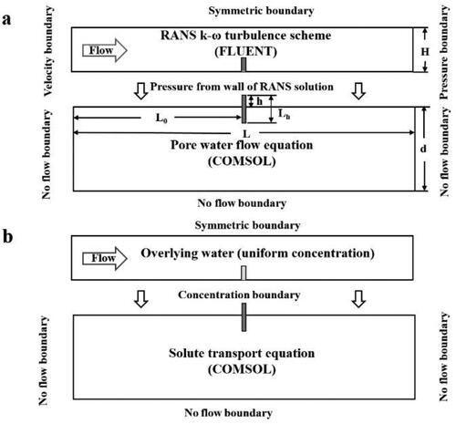
In this study, we assumed the flow to be steady and incompressible, and the bed substrates to be homogeneous, isotropic and free of any shifts. The finite volume-based software FLUENT was used to simulate steady state, two-dimensional turbulent flow over the streambed. The boundary conditions of the model were showed in Figure 2(a). The flow is governed by the continuity equation and Reynolds-averaged Navier-Stokes (RANS) equations, the previous publications used exactly the same simulation (Cardenas and Wilson 2007; Cardenas et al. 2008). For an incompressible fluid, the steady state RANS equations are defined as: (1) $$\frac{\partial {\rho U}_i}{\partial x_i}=0$$(1) (2) $$\rho \frac{\partial U_i}{\partial t}+\frac{\partial \rho U_i{U}_j}{\partial x_j}=-\frac{\partial P}{\partial x_i}+\frac{\partial }{\partial x_j}(2\mu S_{ij}-\rho \overline{{\mu \mathrm{\prime }}_i{\mu \mathrm{\prime }}_j})$$(2) where $\rho$ and μ refer to the fluid density and the dynamic viscosity (assumed standard for water) respectively, U_i or U_j (i, j = 1, 2, where i≠ j) refers to the time-averaged velocity, u^′_i refers to the fluctuations in the instantaneous velocity components in x_i or _j (i, j = 1, 2, where i≠ j) directions, and P refers to the time-averaged pressure. The strain rate tensor (Sij) is defined as: (3) $$S_{ij}=\frac{1}{2}\left[\frac{\partial U_i}{\partial x_j}+\frac{\partial U_j}{\partial x_i}\right]$$(3)

Figure 2. Schematic of the simulation domain and boundaries. Arrows in each figure indicate flow directions. Domains are vertically truncated with only the lowermost portion of the water column and the uppermost portion of the sediments shown. (a) Hydraulics model domain and associated boundaries for the turbulent flow in CFD and groundwater flow in Comsol. L, L₀, H, d, h and L_h are bedform length, distance between weir and boundary, average water depth of overlying water, depth of streambed, the height of the weir, the length of the weir, respectively. (b) For solute transport. Uniform concentration is assumed in the overlying water. The total quantity of solute in the overlying water and the pore water did not vary with time in the flume experiment but the concentration in the overlying water did. For the purpose of simplicity, the solute concentration in the overlying water was kept constant (2.0 g/L). The governing equations are solved sequentially in the following order: (1) RANS k-w, (2) groundwater flow equation, and (3) solute advection–diffusion–dispersion.

The Reynolds stresses are related to turbulent kinetic energy (k) and specific dissipation rate $\omega$ by: (4) $${\tau }_{ij}=-\overline{{{\mu }^{\mathrm{\prime }}}_i{{\mu }^{\mathrm{\prime }}}_j}=v_t\left(2S_{ij}\right)-\frac{2}{3}{\sigma }_{ij}k$$(4) where $v_t$ refers to the kinematic eddy viscosity, ${\sigma }_{ij}$ refers to the Kronecker delta, and k refers to the turbulent kinetic energy.

The eddy viscosity in this closure scheme is: (5) $$v_t=\frac{k}{\omega }$$(5) where the specific dissipation, $\mathrm{\omega },$ is defined as the ratio of the turbulence dissipation rate $\mathrm{\epsilon }$ to k: (6) $$\mathrm{\omega }=\frac{\epsilon }{\beta \mathrm{*}k}$$(6) where b∗ refers to the closure coefficient.

The steady-state migration equations for k and $\mathrm{\omega }$ are: (7) $$\mathrm{\rho }\frac{\partial \left(U_{j}k\right)}{\partial x_j}=\rho {\tau }_{ij}\frac{\partial U_i}{\partial x_j}-{\beta }^{\mathrm{*}}\rho \omega k+\frac{\partial }{\partial x_j}\left[\right(\mu +{\mu }_t{\sigma }_k\left)\frac{\partial k}{\partial x_j}\right]$$(7) (8) $$\mathrm{\rho }\frac{\partial \left(U_j\omega \right)}{\partial x_j}=\alpha \frac{\rho \omega }{k}{\tau }_{ij}\frac{\partial U_i}{\partial x_j}-\beta \rho {\omega }^2+\frac{\partial }{\partial x_j}\left[\right(\mu +{\mu }_t{\sigma }_{\omega }\left)\frac{\partial \omega }{\partial x_j}\right]$$(8)

The standard closure coefficients for the k-w scheme are from Wilcox (2006): a = 5/9, b = 3/40,

${\mathrm{\beta }}^{\mathrm{*}}$= 9/100, and ${\sigma }_k$ = ${\sigma }_{\omega }$ = 0.5.

The simulation domain was then discretized by unstructured grids with quadrilateral mesh elements. The grid was refined near the sediment-water interface. There were 230,000 elements within the simulation domain. FLUENT uses a time-marching scheme together with iteration to solve the steady flow problem. Iterations proceeded until the steady state solution was reached, which was presumed to occur when the maximum relative difference between the computed flow variables (including the averaged flow velocity, pressure, turbulent kinetic energy and turbulence dissipation rate) of two consecutive iteration steps dropped below 10⁻⁵ (Jin et al. 2010).

2.2.2. Mathematical model and boundary conditions for porous flow in sediment

COMSOL Multiphysics, a finite element-based software (Sawyer and Cardenas 2009), was used to simulate numerically flow and solute transport in the bed (Figure 2b). Two-dimensional porous flow in sediment was solved using the steady state groundwater flow equation: (9) $$\frac{\partial }{\partial x_i}\left(-\frac{k}{\mu }\frac{\partial P}{\partial x_i}\right)=0$$(9) where P is the pressure, k is the intrinsic sediment permeability, and $\mu$ is the fluid viscosity. Darcy velocity or groundwater flux q equals the term in brackets. Pressure at the sediment-water interface was specified from turbulent open-channel flow simulation. The lateral and bottom boundaries were shown in Figure 2. In all simulations, the sediment was homogeneous and isotropic.

The solute migration model was established based on the advection-diffusion-dispersion equation for the solute transport: (10) $$\frac{\partial C}{\partial t}=D_m\frac{{\partial }^{2}C}{\partial x_i^2}+\frac{\partial }{\partial x_i}\left(D_{ij}\frac{\partial C}{\partial x_i}\right)-{\mu }_i\frac{\partial C}{\partial x_i}$$(10) where C is the solute concentration, t is time, D_m is the molecular diffusion coefficient in porous media, and D_ij is the mechanical dispersion coefficient tensor, index i, j = 1, 2. The equation for obtaining D_ij is: (11) $$D_{ij}={\alpha }_{T}U{\delta }_{ij}+\left({\alpha }_L-{\alpha }_T\right){\mu }_i{\mu }_j/U$$(11) where ${\mathrm{\alpha }}_{\mathrm{T}}$ and ${\mathrm{\alpha }}_{\mathrm{L}}$ are the transverse and longitudinal dispersivities, ${\mathrm{\alpha }}_{\mathrm{L}}$ was 1 cm (several grain diameters), and ${\alpha }_T$ was 1/10 of ${\mathrm{\alpha }}_{\mathrm{L}}$ (Sawyer et al. 2011). U is the pore velocity magnitude, and ${\delta }_{ij}$ is the Kronecker delta function.

For the purpose of simplicity, we assigned the top boundary (SWI) as a concentration, and the solute concentration in the overlying water in these simulations was assigned constant normalized concentration (C/C₀) of 1.0. Flume walls were assigned zero-flux boundaries. The initial solute concentration in the sediment was zero. The simulation domain was then discretized using structured grids with free triangle mesh elements. The grid was refined near the SWI and the tank wall. There were 1.2 × 10⁵ elements within the simulation domain. Table 1 summarizes the parameters used in the proposed calculation model.

Table 1. Parameters used in the calculation model.

Fluid density ρ (kg·m^−3)	Kinematic eddy viscosity νt (m^2·s^−1)	Porosity θ (%)	Permeability κ (m^2)	Molecular diffusion coefficient Dm (m^2·s^−1)
10^3	1.0 × 10^−6	60	1 × 10^−9	5.0 × 10^−11

2.3. Model evaluation

The root mean square error (RMSE), coefficient of determination (R²), and the relative error (Re) were used to quantitatively evaluate the accuracy of the calculation model: (12) $$\mathrm{RMSE}=\frac{\sqrt{\sum _{i=1}^n{\left(O_i-S_i\right)}^2}}{n}$$(12) (13) $$R^2=1-\sum _{i=1}^n\frac{{\left(O_i-S_i\right)}^2}{\sum _{i=1}^n{O}_i^2}$$(13) (14) $$\mathrm{Re}=\sqrt{\sum _{i=1}^n\frac{{\left(O_i-S_i\right)}^2}{\sum _{i=1}^n{O}_i^2}}$$(14) where O_i, S_i, n, and O refer to the measured value, simulated value, sample size, and average value, respectively. The consistency between the measured and simulated values was measured using RMSE to verify the model. The RMSE is a non-negative value, with a low RMSE indicating a good consistency between the measured and simulated values (Ren et al. 2019). R² is the coefficient of determination of the linear regression equation (y = x) between the measured and simulated values, where a large R² indicates a good consistency between the measured and simulated values (Quinino et al. 2013), Re is the relative error between the measured and simulated values, where a low Re indicates a good consistency between the measured and simulated values (Suñé and Carrasco 2005).

3. Results

3.1. Model validation

The consistency between the measured and simulated values was measured using RMSE to verify. The average flow velocity was 0.04 m·s⁻¹, and the calibrated model was further validated by using data obtained at monitoring periods (30 min, 60 min, 120 min, 180 min, 300 min), as shown in Table 2. Table 2 shows the results of the evaluation of the model simulation accuracy. A close correlation between the observed and measured values was found, in monitoring section N1, with RMSEs of 0.0011–0.0073 m·s⁻¹, which were significantly lower than the average concentration; the R² values were 0.9061–0.9954; and Re was in a reasonable range of 0.23–1.08%. In monitoring section N2, the RMSEs at monitoring periods ranging between 0.001–0.0064 m·s⁻¹, which were significantly lower than the average concentration; R² at monitoring periods ranging between 0.8413–0.9620; and Re was 0.12–1.64%. In summary, the proposed model exhibited an excellent simulation accuracy and can precisely describe the dynamic migration of bed solutes.

Table 2. Accuracy of vertical simulation of the solute concentrations at different monitoring points and periods.

Monitoring sections	Monitoring periods (min)	RMSE (m·s^−1)	R^2	Re (%)
N1	30	0.0073	0.9061	1.08
	60	0.0039	0.9388	0.56
	120	0.0011	0.9688	0.13
	180	0.0022	0.9943	0.25
	300	0.0019	0.9954	0.23
N2	30	0.0021	0.9540	1.64
	60	0.0018	0.9620	1.35
	120	0.0064	0.8413	1.25
	180	0.001	0.9140	0.12
	300	0.0041	0.9122	0.45

3.2. Simulated channel velocity fields, interfacial pressures, and velocity

The numerical simulations showed that surface water accelerated around the weir, the maximum velocity approached 40–50 cm/s around the top of the weir. At the rear end of the weir, the flow velocity gradually decreased, and the minimum velocity value was below 8 cm/s. Moreover, there was an obvious vortex downstream of the weir (Figure 3a). The overall patterns of the pressure distributions along the SWI showed that the weir created counter-acting forces of increased downwelling head due to backwater effects, where a local pressure maxima occurred on the upstream of the weir, and increased upwelling due to low streambed pressure and standing waves downstream of the structure, and pressure recovered approximately 0.3 m downstream of the weir (Figure 3b).

Figure 3. (a) Simulated flow rates of the surface water and pore water, as well as (b) interfacial pressures and (c) velocity (vertical velocity). Channel flow is left to right. Thin black lines indicate streamlines. The red arrow lines represent the flow fields.

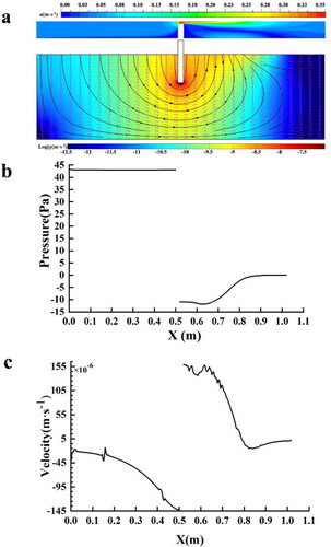
The status of the velocity field distributions along the SWI was similar to the pressure distributions. The maximum downwelling rate was 0.14 mm·s⁻¹ and occurred less than 1 cm upstream of the weir’s leading edge, and the maximum upwelling rate was 0.16 mm·s⁻¹ and immediately occurred 5 cm downstream of the weir center. The average flow rate across the SWI was 0.004 mm·s⁻¹. The peculiar velocity field generally caused downwells in two locations: upstream of the weir, and away from the downstream of the weir, leading the various spatial distributions of hyporheic exchange cells (Figure 3c). In addition, the simulation delineated upwelling flow paths converge strongly near the downstream of the weir, curving back upstream somewhere. The small, shallow cell of secondary exchange cell beneath the wake zone downstream of the weir and deflected flow paths. This was caused by the pressure gradients distribution of the SWI. Nevertheless, because the depth of the cell and exchange rates within it were small, the cell should not significantly impact solute transport within the sediment. The fastest fluxes occur beneath the weir and decay rapidly with distance upstream and downstream, and the spatial extent of hyporheic exchange was limited only by the flume walls.

3.3. Spatial and temporal variations of solute concentrations in the bed

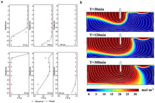
As mentioned, several vertical arrays of sampling ports were installed to monitor the variation of solute concentration in the pore water. Array N1 was located at the upstream of the weirs where the solute entered the streambed, and array N2 was located at the downstream of the weirs where the solute exited the streambed. The distinction between these sampling areas was thought to be important for studying the solute transport behaviour under the influence of circulation induced by weir interactions. The depth profiles of the measured solute concentration at sampling locations and various times were displayed in Figure 4(b), where they were compared with the model predictions. The results from numerical simulations with the measured values were compared, overall the model simulated the observations well (Figure 4a). These profiles appeared to show a solute front propagating downward at arrays N1 and N2. However, the weir altered pore water flow patterns, resulting in more rapid downward movement of the solute front at the upstream of the weir. Meanwhile, this phenomenon did not simply reflect a downward solute movement but resulted from both horizontal (e.g. from N1 to N2) and vertical solute transport through pore water circulation cells. For example, the concentration at a deep port of N2 would not correspond to the concentration in the shallow area (ports above) of this sampling location. Instead, it was related to the concentration near a port of N1 given that both ports were along the same circulation path. In general when the solute front passed through the upstream of the weir to the downstream, the magnitude and direction of the pore water flow were modified due to the weir. It is also evident that higher solute concentrations at deeper ports of N1 and N2 at a particular time were linked to higher solute concentrations in the overlying water at earlier times; however, the deeper ports were associated with longer and slower paths and lower circulation at later times. It is also worth noting that, as time went on, the maximum concentration over the depth at both N1 and N2 slightly decreased, occurring deeper in the array. This behavior corresponds to a hyporheic exchange between the overlying water and the pore water, which induced the reduction of the solute concentration in the overlying water with time. These phenomena were partly due to solute dispersion.

Figure 4. (a) Comparison between the measured (hollow squares) and predicted (red curves) solute concentrations varying with depth. (b) Solute concentration distribution at different times. The color scale for the outputs (b), representing solute concentration; warmer colors: higher concentration, cooler colors: lower concentration. White lines show flow directions (but not magnitude) in the porous media. No vertical exaggeration. Channel flow is left to right.

4. Discussion

Summarizing the previous literature, a variety of factors were inferred to have a remarkable influence on hyporheic exchange. Among them, the structure size (Hester and Doyle 2008; Liu and Chui 2020), sediment intrinsic permeability (Ward et al. 2011; Herzog et al. 2016) and hydrological condition (Sawyer et al. 2011; Ren et al. 2019) were the most important factors. The primary objective of this study was to determine the independent effect of a wide range of potential controls on the vertical hyporheic exchange flux and the maximum solute front penetration depth induced by a single weir. This was accomplished through a sensitivity analysis where each of the parameters of interest was varied separately. The factors that varied included the structure size (h, just above the streambed), sediment intrinsic permeability (k) and velocity (u) (Table 3). When each factor was varied, all remaining factors were held constant at base case values.

Table 3. Various parameters in the sensitivity analysis.

Factor level	h (cm)	u (m•s^−1)	k (m^2)
1	1	0.04	10^−8
2	2	0.08	10^−9
3	3	0.12	10^−10
4	4		10^−11
5	5		10^−12

4.1. Effect of the structure size-induced hyporheic exchange

As structure size was a critical factor in determining the relationship between the weir morphology and hyporheic exchange, meanwhile, the size of the weir was controllable for the restoration project. In this study, hyporheic exchange at weir heights h = 1 cm, 2 cm, 3 cm, 4 cm and 5 cm was investigated. The staggered pressure distribution caused by the weir morphology was the main driving force of hyporheic exchange. Figure 5(a) showed that the pressure distributions along the SWI for different weir heights. The pressure distribution patterns were much similar, pressure along the SWI in generally slightly decreased downward upstream of the weir; and increased upward downstream of the weir. However, the pressure tended to increase in magnitude with the weir height. Meanwhile, the height of the weir strongly affected the velocity distribution and the magnitude. The velocity distribution patterns along the SWI were uniform, and the distribution of upwelling and downwelling flow on the SWI essentially maintained the same change; in general, the velocity rate tended to increase in magnitude with the weir height (Figure 5b).

Figure 5. (a) Pressure and (b) velocity rate along the sediment-water interface for different weir heights (different colour lines represent schematically different weir heights). The log center is at x = 0.51 m. Simulations of hyporheic fluid flow predict similar patterns upstream and downstream of the weir. Flow in the overlying water column (not shown) is from left to right.

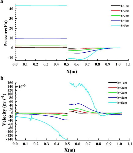
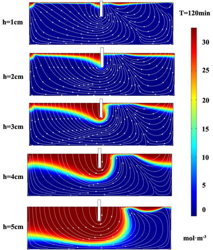
To further analyze the effects of weir’s height on hyporheic exchange, the solute penetration depth at different weir heights was further investigated. Figure 6 shows that as the weir height increased, the depth and range of hyporheic exchange of solutes per unit time showed a positive relationship with heights due to interactions of the surface water and subsurface water. The solute front depth (D_p) penetrated to the deepest below the weir and shrunk to its shallowest point downstream of the weir, due to a hydraulic jump with a low streambed pressure forming downstream of the structure. Otherwise, for h = 1 cm, 2 cm, 3 cm, 4 cm and 5 cm, the maximum D_p were 3 cm, 8 cm, 13 cm, 18 cm and 27 cm respectively.

Figure 6. Solute transport fluxes in the streambed for cases with different h at T = 120 min. The color scale for the outputs represents solute concentration; warmer colors: higher concentration, cooler colors: lower concentration. White lines show flow directions (but not magnitude) in the porous media. No vertical exaggeration. Flow in the overlying water column (not shown) is from left to right.

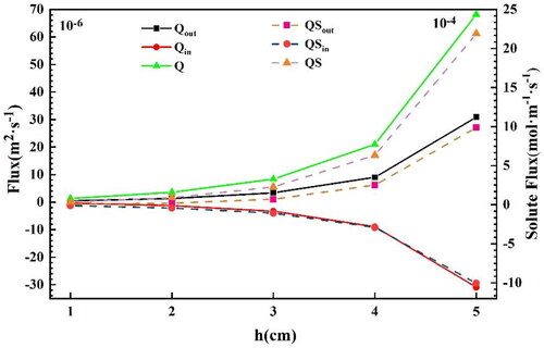
The magnitude of the vertical flux and solute flux induced by a weir could be viewed as decisive metrics of hyporheic exchange. The relationships between the weir height and the hyporheic exchange flux metrics were of similar shape for different weir heights; as the weir height increased, the upwelling flux (4.22 × 10⁻⁷–3.09 × 10⁻⁵ m²·s⁻¹) and downwelling flux (−3.86 × 10⁻⁷–3.09 × 10⁻⁵ m²·s⁻¹) increased exponentially (Figure 7). Although the Q increases slowly, it also increases exponentially (from 1.33 × 10⁻⁶–6.82 × 10⁻⁵ m²·s⁻¹), which was consistent with Hester and Doyle (2008) and Sawyer et al. (2011), who found an increase in the downwelling flux with head drop across a log. This increase in the head drop was analogous to an increase in the weir height in our modeling study, because increasing the weir height increased in-stream head drop and associated hyporheic Darcy flux processes due to channel steepening, backwater, and/or form drag mechanisms. In fact, this connection between the structure size, head drop, and induced hyporheic flux could be understood by applying Darcy’s Law to the hyporheic flow originating within the patch-scale area. Because the weir height was varied in this study under the conditions of constant K, Darcy’s Law can be simplified: (15) $$\mathrm{Q}=\mathrm{K}\frac{\Delta h}{l}A$$(15) where A is the cross-sectional area of the subsurface (hyporheic) flow path and $\Delta \mathrm{h}$ is the in-stream head drop across the structure. Because the relationships between the interface pressure drop which has a positive relation with $\Delta \mathrm{h}$ and the weir height have the same trend as the relationships between Q and the weir height (Figure 7), it is clear that $\Delta \mathrm{h}$ in Eq. (1)(1) $$\frac{\partial {\rho U}_i}{\partial x_i}=0$$(1) is more important than A or l in determining Q and that the in-stream structure controls Q primarily by controlling the interface pressure drop and $\Delta \mathrm{h}.$ Furthermore, the metric of QS had the same trend, but the total solute flux increased from 3.54 × 10⁻⁵–2.19 × 10⁻³mol·m⁻¹·s⁻¹. In other words, the magnitude of Q and QS had a positive exponential relationship with the weir height; however, h had no effect on any hyporheic zone metric for an h of 3 cm or less, that was, the values of flux, while substantial, reflected the minimum size of the most effective type of the weir.

Figure 7. Vertical hyporheic exchange flux (Q), downwelling hyporheic flux (Q_in), upwelling hyporheic flux (Q_out), solute flux (QS), downwelling solute flux (QS_in) and upwelling hyporheic flux (QS_out) in the streambed for cases with different h values. The solid lines represent the hyporheic flow flux; the dashed lines show the solute flux.

4.2. Effect of velocity-induced hyporheic exchange

The hydrogeologic context of the stream was generally important in determining the degree of hyporheic exchange induced by the weir, but this importance varied among specific contextual parameters. Stream velocity (u) had a substantial effect on all hyporheic exchange metrics that was consistent across weir heights (Figure 8). We kept the height of the weir (as well as other factors) at a constant value (h = 5 cm). Figure 8(a) showed that the pressure distribution pattern was very similar along the SWI for different velocities. However, the pressure tended to increase in magnitude with the velocity rate.

Figure 8. (a) Pressure and (b) vertical hyporheic exchange flux (Q), downwelling hyporheic flux (Q_in), upwelling hyporheic flux (Q_out), solute flux (QS), downwelling solute flux (QS_in) and upwelling hyporheic flux (QS_out) in the streambed for cases with different u values. The solid lines represent the hyporheic flow flux; the dashed lines show the solute flux. (c) Solute transport fluxes in the streambed for cases with different u at T = 120 min. The color scale for the outputs represents solute concentration; warmer colors: higher concentration, cooler colors: lower concentration. White lines show flow directions (but not magnitude) in the porous media. No vertical exaggeration. Flow in the overlying water column (not shown) is from left to right.

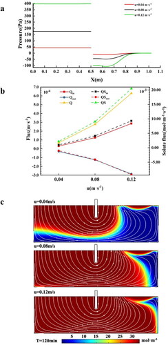
To further analyse the effects of the velocity rate on hyporheic exchange, the solute penetration depth at different velocity rates was further explored. Figure 8(c) showed that as velocity rate increased, the depth and range of hyporheic exchange of solutes per unit time showed a positive relationship with the velocity rate due to more intense interactions of the surface water and subsurface water, D_p for u = 0.04 m·s⁻¹, 0.08 m·s⁻¹, and 0.12 m·s⁻¹ differed sharply. And at the same time scale (T = 120 min), D_p was shallower at the lower flow rate (u = 0.04 m·s⁻¹); while at higher velocity, the material had already penetrated to the bottom boundary.

The simulations results showed that the hyporheic vertical exchange flux, solute flushing and penetration depth were consistently influenced by the multiple velocity rates (Figure 8b). As the stream velocity increased, it produced a much larger pressure drop, and Q and QS across the bed were greatly increased. Although Q, the upwelling flux and downwelling flux rate increased exponentially with velocity, but the overall growth was slowly, Q increased from 6.82 × 10⁻⁵ to 6.29 × 10⁻⁴ m²·s⁻¹, and the upwelling flux and downwelling flux rate increased from 3.09 × 10⁻⁵ to 2.86 × 10⁻⁴ m²·s⁻¹, and from −3.09 × 10⁻⁵ to 2.86 × 10⁻⁴ m²·s⁻¹, respectively. Meanwhile, QS had the same trend, but the total solute flux increased from 2.19 × 10⁻³ to 2.05 × 10⁻² mol·m⁻¹·s⁻¹. This result was reasonable because a higher velocity entails greater rates of pressure drop and Darcy flux within the streambed, which would tend to be consistent with the structure-induced hyporheic flux. An important implication was that although in-steam velocity measurably impacts hyporheic exchange, hyporheic exchange flux and solute penetration depth increased less rapidly. This was consistent with Zhou and Endreny (2013), who noted that the restoration structures generated backwater effects that increased downwelling forces; however, these forces were nearly counter-balanced by low bed pressures downstream of the structure, where the balance of these forces shifted and low bed pressures caused moderate growth in response of hyporheic exchange.

4.3. Effect of sediment intrinsic permeability (k)-induced hyporheic exchange

In addition to geometry, the sediment intrinsic permeability k is a significant control of the weir structure performance. For brevity, the porosity was set to 0.6 and was not varied with k in order to focus our analysis on variability of k itself. Meanwhile, we kept the height of the weir (as well as other factors) to be a constant value (h = 5 cm). The weir-induced hyporheic hydraulics we simulated fundamentally shifted k from 10⁻⁸–10⁻¹² m² (that is, the streambed material changes from gravel to fine sand). We delineated the process of hyporheic exchange separately for each k by only focusing on the metrics of flux that both downwelled from and upwelled to the channel and the solute front depth that penetrated subsurface. Hyporheic exchange was generally the most sensitive to changes in k in terms of both the metrics of flux and the solute front penetration depth (Figure 9); that was, the increased sediment intrinsic permeability (k) significantly affected the exchange, inducing increases in the water flux and solute flux. The impact of k on flux was consistent with Darcy’s Law (Eq. (15)(15) $$\mathrm{Q}=\mathrm{K}\frac{\Delta h}{l}A$$(15) ), which indicated that Q was proportional to k, where $\Delta \mathrm{h},$ l, and A were constant, yielding an exponential relationship. Similarly, as Q increased, the depth of the solute front penetration along the entire wavelength typically increased, where the flux increased exponentially.

Figure 9. (a) Solute transport fluxes in the streambed for cases with different k at T = 120 min. The color scale for the outputs represents solute concentration; warmer colors: higher concentration, cooler colors: lower concentration. White lines show flow directions (but not magnitude) in the porous media. No vertical exaggeration. Flow in the overlying water column (not shown) is from left to right. (b) Vertical hyporheic exchange flux (Q), downwelling hyporheic flux (Q_in), upwelling hyporheic flux (Q_out), solute flux (QS), downwelling solute flux (QS_in) and upwelling hyporheic flux (QS_out) in the streambed for cases with different k. The solid lines represent the hyporheic flow flux; the dashed lines show the solute flux.

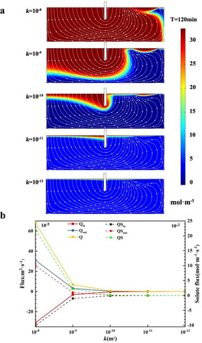
However, k had no effect on any hyporheic zone metric for a k value of 10⁻¹¹ m/s or less (Figure 9). These results generally agreed with those of Storey et al. (2003) and Ward et al. (2011) for the downwelling flux and hyporheic depth and the flux across much of the range of k. Contrary to our findings, Lautz and Fanelli (2008) reported that the hyporheic volume increased with k, but they defined the hyporheic zone ‘hydrochemically’, which was dependent on transport parameters (some of which can vary with k), and their site was heterogeneous with respect to k. Overall, our results imply that hyporheic zones in areas with a coarser substrate (e.g. steep mountainous regions, glacial outwash) may have greater downwelling flux rates and hyporheic depth, whereas areas with finer substrates (e.g. lower gradient plains or coastal regions) may have less of a hyporheic flux, as well as hyporheic depth.

5. Summary and conclusions

Hyporheic exchange is increasingly recognized as important in streams and rivers due to the significant ecological consequences it provides. In this study, we conducted flume experiments with solute injection to investigate how in-stream structures impact the response of hyporheic exchange, which was quantified with the vertical hyporheic exchange flux and maximum solute front penetration depth. These variables were either observed or derived from the flume experimental data and were used to verify the combination of the multiphysics computational fluid dynamics (CFD) approach and COMSOL Multiphysics simulations. The validated COMSOL Multiphysics model was then applied as a virtual flume to investigate the impacts of the height of the in-stream weir, the in-flow velocity rate and sediment intrinsic permeability k on hyporheic exchange. The major findings were as follows:

The coupling mathematical numerical model simulations were verified against observations using the RMSE, R², and Re as evaluation indices. In summary, the simulation results were highly consistent with the experimental results; therefore, it was argued that the proposed calculation model was reliable.

A multidimensional modeling approach was rigorously evaluated hyporheic response to a suite of controlling factors associated with the weir. The analysis results yielded that the vertical hyporheic exchange and the maximum solute front penetration depth generally increased with the weir height until it was constrained by geologic, or hydrologic constraints.

Hydrologic setting conditions appeared to be important, with an increased channel velocity tending to impact hyporheic exchange; nonetheless, the hyporheic exchange flux and solute penetration depth increased less rapidly.

Meanwhile, the exchange metric of interest was dependent on the impact of the intrinsic permeability k. As predicted by a straight forward application of Darcy’s Law, the magnitude of the hyporheic flux had an exponential relationship with the sediment hydraulic conductivity. However, k had no effect on any hyporheic zone metric for k value of 10⁻¹¹ m/s or less.

In general, our model for bed pressure profiles and the response of hyporheic exchange in the vicinity of the weir can be used to inform the design of in-stream structure restoration projects. Meanwhile, how these structures of different settings (size, number) and hydrogeologic metrics combine to influence the exchange between the stream and substratum remains an important question for future research. Follow-on work should explore other vertical factors that influence hyporheic exchange rate and the maximum solute penetration depth. Factors of interest include (1) the flow depth, (2) the placement and geometry of the restoration structures, including the number and gaps of obstacles, and (3) the streambed hydraulically heterogeneous and anisotropic. Variations in these factors would potentially change the pattern and magnitude of the hyporheic flow and consequently influence the degree of mixing. A multidimensional modeling approach is necessary to rigorously evaluate the hyporheic response to a suite of controlling factors associated with weirs.

Acknowledgments

We thank the editor and reviewers for constructive comments on the manuscript. We are grateful to the National Natural Science Foundation of China (52179131, 41902248), and the Open Research Foundation of Key Laboratory of the Pearl River Estuarine Dynamics and Associated Process Regulation, Ministry of Water Resources ([2017]KJ08).

Disclosure statement

This manuscript has not been published or presented elsewhere in part or entirety and is not under consideration by another journal. There are no conflicts of interest to declare.

Additional information

Funding

This work was supported by National Natural Science Foundation of China (52179131, 41902248), and the Open Research Foundation of Key Laboratory of the Pearl River Estuarine Dynamics and Associated Process Regulation, Ministry of Water Resources ([2017]KJ08).

Notes on contributors

Jinghong Feng

Jinghong Feng is a doctoral graduate student at College of Hydraulic and Environmental Engineering, China Three Gorges University, Yichang, China. She focus on ecological restoration projects of small and medium rivers.

Defu Liu

Defu Liu is a professor at Hubei Key Laboratory of Ecological Restoration of River-lakes and Algal Utilization, Hubei University of Technology. He focus on Eco-hydraulic engineering for many years.

Ying Liu

Ying Liu, PhD, is an Associate Professor at Hubei Key Laboratory of Ecological Restoration of River-lakes and Algal Utilization, Hubei University of Technology. She focus on ecological restoration projects of small and medium rivers.

Yi Li

Yi Li, PhD, is an Associate Professor at Hubei Key Laboratory of Ecological Restoration of River-lakes and Algal Utilization, Hubei University of Technology. He focus on seepage simulation of underground multi-component multiphase flow.

Han Li

Han Li is a master degree candidate who is studying in Hubei Key Laboratory of Ecological Restoration of River-lakes and Algal Utilization, Hubei University of Technology.

Lihui Chen

Lihui Chen is a master degree candidate who is studying in Hubei Key Laboratory of Ecological Restoration of River-lakes and Algal Utilization, Hubei University of Technology.

Jingwen Xiao

Jingwen Xiao is a master degree candidate who is studying in Hubei Key Laboratory of Ecological Restoration of River-lakes and Algal Utilization, Hubei University of Technology.

Jixin Liu

Jixin Liu is a master degree candidate who is studying in Hubei Key Laboratory of Ecological Restoration of River-lakes and Algal Utilization, Hubei University of Technology.

Jiawei Dong

Jiawei Dong is a master degree candidate who is studying in Hubei Key Laboratory of Ecological Restoration of River-lakes and Algal Utilization, Hubei University of Technology.

References

- Azinheira DL, Scott DT, Hession W, Hester ET. 2014. Comparison of effects of inset floodplains and hyporheic exchange induced by in-stream structures on solute retention. Water Resour Res. 50(7):6168–6190.
- Boulton AJ. 2007. Hyporheic rehabilitation in rivers: restoring vertical connectivity. Freshwater Biol. 52(4):632–650.
- Boulton AJ, Datry T, Kasahara T, Mutz M, Stanford JA. 2010. Ecology and management of the hyporheic zone: stream-groundwater interactions of running waters and their floodplains. J North Am Benthol Soc. 29(1):26–40.
- Boulton AJ, Findlay S, Marmonier P, Stanley EH, Valett HM. 1998. The functional significance of the hyporheic zone in streams and rivers. Annu Rev Ecol Syst. 29(1):59–81.
- Buchanan B, Walter M, Nagle G, Schneider R. 2012. Monitoring and assessment of a river restoration project in central New York. River Res Appl. 28(2):216–233.
- Cardenas MB. 2006. Dynamics of fluids, heat and solutes along sediment–water interfaces: a multiphysics modeling study [Ph.D. thesis]. The New Mexico Institute of Mining and Technology.
- Cardenas MB, Wilson JL. 2007. Dunes, turbulent eddies, and interfacial exchange with permeable sediments. Water Resour Res. 43(8):199–212.
- Cardenas MB, Wilson JL, Haggerty R. 2008. Residence time of bedform-driven hyporheic exchange. Adv Water Resour. 31(10):1382–1386.
- Chin A, Anderson S, Collison A, Ellis-Sugai BJ, Haltiner JP, Hogervorst JB, Kondolf GM, O’Hirok LS, Purcell AH, Riley AL. 2009. Linking theory and practice for restoration of step-pool streams. Environ Manage. 43(4):645–661.
- Daniluk TL, Lautz LK, Gordon RP, Endreny TA. 2013. Surface water-groundwater interaction at restored streams and associated reference reaches. Hydrol Process. 27(25):3730–3746.
- Elliott AH. 1990. Transfer of solutes into and out of streambeds. Rep KH-R-52, WM Keck Lab Hydraul Water Resour, Calif Inst Technol, Pasadena, USA.
- Endreny T, Lautz L, Siegel D. 2011a. Hyporheic flow path response to hydraulic jumps at river steps: flume and hydrodynamic models. Water Resour Res. 47:W02517.
- Findlay S. 1995. Importance of surface-subsurface exchange in stream ecosystems: the hyporheic zone. Limnol Oceanogr. 40(1):159–164.
- Gordon RP, Lautz LK, Daniluk TL. 2013. Spatial patterns of hyporheic exchange and biogeochemical cycling around cross-vane restoration structures: implications for stream restoration design. Water Resour Res. 49(4):2040–2055.
- Hancock PJ. 2002. Human impacts on the stream-groundwater exchange zone. Environ Manage - New York. 29(6):763–781.
- Hancock PJ, Boulton AJ, Humphreys WF. 2005. Aquifers and hyporheic zones: towards an ecological understanding of groundwater. Hydrogeol J. 13(1):98–111.
- Harvey JW, Gooseff M. 2015. River corridor science: hydrologic exchange and ecological consequences from bedforms to basins. Water Resour Res. 51(9):6893–6922.
- Harvey JW, Wagner BJ. 2000. Quantifying hydrologic interactions between streams and their subsurface hyporheic zones. Streams and Ground Waters: Academic Press, USA. p. 3–44.
- Herzog SP, Higgins CP, Mccray JE. 2016. Engineered streambeds for induced hyporheic flow: enhanced removal of nutrients, pathogens, and metals from urban streams. J Environ Eng. 142(1):04015053.
- Hester ET, Doyle MW. 2008. In-stream geomorphic structures as drivers of hyporheic exchange. Water Resour Res. 44(3):893–897.
- Hester ET, Doyle MW, Poole GC. 2009. The influence of in-stream structures on summer water temperatures via induced hyporheic exchange. Limnol Oceanogr. 54(1):355–367.
- Hester ET, Gooseff MN. 2010. Moving beyond the banks: hyporheic restoration is fundamental to restoring ecological services and functions of streams. Environ Sci Technol. 44(5):1521–1525.
- Hester ET, Gooseff MN. 2013. Hyporheic restoration in streams and rivers, in stream restoration in dynamic fluvial systems. Washington, DC: American Geophysical Union.
- Jiang QH, Jin GQ, Tang HW, Shen CJ, Cheraghi M, Xu JZ, Li L, Barry DA. 2020. Density-dependent solute transport in a layered hyporheic zone. Adv Water Resour. 142:103645.
- Jin GQ, Tang HW, Gibbes B, Li L, Barry DA. 2010. Transport of nonsorbing solutes in a streambed with periodic bedform. Adv Water Resour. 33(11):1402–1416.
- Krause S, Hannah DM, Fleckenstein JH. 2009. Hyporheic hydrology: interactions at the groundwater-surface water interface preface. Hydrol Process. 23(15):2103–2107.
- Lautz LK, Fanelli RM. 2008. Seasonal biogeochemical hotspots in the streambed around restoration structures. Biogeochemistry. 91(1):85–104.
- Lautz LK, Siegel DI, Bauer RL. 2006. Impact of debris dams on hyporheic interaction along a semi-arid stream. Hydrol Process. 20(1):183–196.
- Lewandowski J, Arnon S, Banks E, Batelaan O, Betterle A, Broecker T, Coll C, Drummond JD, Garcia JG, Galloway J, et al. 2019. Is the hyporheic zone relevant beyond the scientific community? Water. 11(11):2230.
- Liu S, Chui T. 2020. Optimal in-stream structure design through considering nitrogen removal in hyporheic zone. Water. 12(5):1399.
- Menichino GT, Hester ET. 2014. Hydraulic and thermal effects of in-stream structure-induced hyporheic exchange across a range of hydraulic conductivities. Water Resour Res. 50(6):4643–4661.
- Newbold JD, O’Neill RV, Elwood JW, Van Winkle W. 1982. Nutrient spiraling in streams: implications for nutrient limitation and invertebrate activity. Am Nat. 120(5):628–652.
- Norman FA, Cardenas MB. 2014. Heat transport in hyporheic zones due to bedforms: an experimental study. Water Resour Res. 10(1):29–38.
- Packman AI, Bencala KE. 2000. Modeling methods in the study of surface-subsurface hydrologic interactions. Streams and Ground Waters: Academic Press, USA. p. 45–80.
- Packman AI, Brooks NH, Morgan JJ. 2000. A physicochemical model for colloid exchange between a stream and a sand streambed with bed forms. Water Resour Res. 36(8):2351–2362.
- Quinino RC, Reis EA, Bessegato LF. 2013. Using the coefficient of determination R2 to test the significance of multiple linear regression. Teach Stat. 35(2):84–88.
- Ren J, Packman AI. 2004. Stream-subsurface exchange of zinc in the presence of silica and kaolinite colloids. Environ Sci Technol. 38(24):6571–6581.
- Ren J, Wang X, Zhou Y, Chen B, Men L. 2019. An analysis of the factors affecting hyporheic exchange based on numerical modeling. Water. 11(4):665.
- Rosgen DL. 2001. The cross-vane, W-Weir and J-Hook vane structures… Their description, design and application for stream stabilization and river restoration. Wetlands Engineering & River Restoration. p. 1–22.
- Sawyer AH, Cardenas MB. 2009. Hyporheic flow and residence time distributions in heterogeneous cross-bedded sediment. Water Resour Res. 45(8):W08406.
- Sawyer AH, Cardenas MB. 2012. Effect of experimental wood addition on hyporheic exchange and thermal dynamics in a losing meadow stream. Water Resour Res. 48(10):10537.
- Sawyer AH, Cardenas MB, Buttles J. 2011. Hyporheic exchange due to channel-spanning logs. Water Resour Res. 47(8):427–438.
- Smidt SJ, Cullin JA, Ward AS, Robinson J, Zimmer MA, Lautz L, Endreny TA. 2015. A comparison of hyporheic transport at a cross-vane structure and natural riffle. Groundwater. 53(6):859–871.
- Storey RG, Howard K, Williams DD. 2003. Factors controlling riffle-scale hyporheic exchange flows and their seasonal changes in a gaining stream: a three-dimensional groundwater flow model. Water Resour Res. 39(2):180–189.
- Suñé V, Carrasco JA. 2005. Efficient implementations of the randomization method with control of the relative error. Comput Oper Res. 32(5):1089–1114.
- Swanson TE, Cardenas MB. 2010. Diel heat transport within the hyporheic zone of a pool-riffle-pool sequence of a losing stream and evaluation of models for fluid flux estimation using heat. Limnol Oceanogr. 55(4):1741–1754.
- Tockner K, Pennetzdorfer D, Reiner N, Schiemer F, Ward J. 1999. Hydrological connectivity, and the exchange of organic matter and nutrients in a dynamic river-floodplain system (Danube, Austria). Freshwater Biol. 41(3):521–535.
- Triska FJ, Kennedy VC, Avanzino RJ, Zellweger GW, Bencala KE. 1989. Retention and transport of nutrients in a third-order stream: channel processes. Ecology. 70(6):1877–1892.
- Ward AS, Gooseff MN, Johnson PA. 2011. How can subsurface modifications to hydraulic conductivity be designed as stream restoration structures? Analysis of Vaux’s conceptual models to enhance hyporheic exchange. Water Resour Res. 47(8):W08512.
- Wilcox DC. 2006. Turbulence modeling for CFD (Third Edition). DCW Industries, Incorporated, USA.
- Winter TC, Harvey JW, Franke OL, Alley WM. 1998. Ground water and surface water: a single resource. U.S. Geological Survey Publications. p. 79.
- Zhou T, Endreny TA. 2013. Reshaping of the hyporheic zone beneath river restoration structures: flume and hydrodynamic experiments. Water Resour Res. 49(8):5009–5020.