Theoretical Response of Laser Aerosol Spectrometers and Data Inversion by Stochastic Reconstruction

Abstract

Laser optical particle spectrometers have been used to obtain real-time particle counts and infer mass information over a substantial portion of the PM_2.5 mass range by means of dynamic aerosol calibrations. The theoretical response of such instruments is quite calculable, as many authors have demonstrated, but the total response still has some problem areas. This article addresses the theoretical response, comparing the calculations to the instrument calibration and other experimental data. Other instrument characteristics, particularly the particle path through the instrument, affect the total response. When the whole instrument is considered, theoretical predictions of response with changes of index of refraction can be made with some confidence.

The calculated response of such spectrometers is nonmonotonic with particle size for most indices of refraction, making inversion of the acquired data difficult. A data inversion algorithm has been devised to incorporate all the response effects and overcome the multivalued nature of the response curve. The inversion algorithm simulates particles passing through the instrument, subject to constraints imposed by the instrument (and user) according to the information desired. The inversion technique is robust and should be useful in other aerosol applications as well.

The software algorithm source files mentioned in this article are available online at http://taylorandfrancis.metapress.com/openurl.asp?genre=article&id=doi:10.1080/02786820490439710 To access this file, click on the issue link for 38(5), then select this article. In order to access the full article online, you must either have an institutional subscription or a member subscription accessed through www.aaar.org.

INTRODUCTION

Optical particle counters using laser illumination are widely used in aerosol applications. They have two principal advantages over white-light counters: more intense illumination and a smaller scattering region. The first advantage allows the sizing of smaller particles, while the second allows higher particle concentrations to be measured without coincidence problems. However, the monochromatic nature of the laser causes the light scattering response to be more strongly dependent on particle size and index of refraction than in white-light instruments, whose wavelength averaging smooths the response to size. The laser instrument response may become nonmonotonic with particle size if the size parameter becomes large.

We desired to use a laser particle counter (a Particle Measuring Systems LAS-X) to size titanium dioxide particles, with a high index of refraction, as accurately as possible. The strong resonance structure of theoretical scattering curves for such particles limited the usefulness of calculations until a data inversion technique could be devised that would cope with the nonmonotonic scattering functions.

The LAS-X laser spectrometer is a good application for this type of inversion because its response can be accurately calculated for spherical particles. This means it can be used with aerosols for which there are no calibration standards. Moreover, the same optical system is used in other commercial laser spectrometers (Hiac/Royco Models 226/236, Particle Measuring Systems Model HSLAS and ASASP-X), making calculations adaptable to those instruments with only minor changes. All these instruments use an active laser system in which the particles flow through the laser cavity, and several attempts have been made to compute the theoretical response. Older active laser instruments (Knollenberg, 1979) do not have the same geometry, but the principles of analysis are the same.

Normally, a MIE-scattering calculation would be a straightforward application of scatter light intensities integrated over all the angles that reach the detector. However, within the laser cavity, two oppositely directed beams are incident on each particle. The forward-scattered components from one beam arrive at the detector along with the back-scattered components of the other. The question is, how should the scattered light from both beams be treated at the detector? Should the intensities (proportional to the local electric field squared) of the scattered light from the two beams be added or should the electric fields themselves be added?

The two approaches give qualitatively different answers, with the addition of intensities producing response curves that are much smoother than with the addition of electric fields. Since these instruments were introduced, many experimental measurements have been performed to distinguish the approaches, and many arguments concerning relative phases between the beams or cavity modes have been presented to justify using one or the other method, as summarized below.

At the detector, only the instantaneous electric field is important for producing a current; that is, the fields are always additive. If the electric fields from two separate sources are in a stable phase relationship (identical frequencies), then the addition is proportional only to the cosine of the phase difference between them. If the two sources are at different frequencies, then the detector may respond to the beat frequency difference between them if the difference is not too large. Otherwise, the two electric fields effectively excite the detector independently (because of the rapid phase change of one with respect to the other) and the intensities appear to be additive. In the laser cavity, the two beams in a single mode are definitely at the same frequency, so that addition of the scattering amplitudes (with a possible phase difference) is the appropriate method for computation.

Garvey and Pinnick (1983) and Soderholm and Saltzman (1984) present analyses of the scattering response of an active laser aerosol spectrometer in terms of two plane waves traveling in opposite directions. Garvey and Pinnick do this for particles located at an antinode (maximum intensity) of the laser's standing wave pattern. After integration over the collecting angle of the detector, the size-dependent response is similar to a standard Mie scattering curve, exhibiting a monotonically increasing response to size until the first resonance and an increasingly complex response with multiple resonances above that. They presented some experimental measurements on Polystyrene Latex (PSL) spheres and nigrosin dye spheres and found good agreement with the coherent wave results. They also found equally good agreement with incoherent wave results. The scatter in the experimental data contributed most of the uncertainty, however.

Soderholm and Saltzman discussed results of many calculations, averaging over all possible positions of particles in the standing wave pattern. They concluded that the incoherent addition of the scattered waves is an appropriate description of the laser spectrometer.

However, in our judgment, a single particle passes through the beam at one particular location in the standing wave pattern, and when it does, the scattered components are in a stationary phase relationship at the detector. Thus the scattering should still be correlated. With the passage of multiple particles, the relative phase would vary from position to position. The coherent response from each particle with these phase differences should be averaged appropriately to determine the overall instrument response.

Szymanski and Liu (1986) experimentally investigated the sizing accuracy of two different laser-based instruments and observed that the experimental size response was smoother than the calculations reported by Garvey and Pinnick. Nonetheless, they observed index-of-refraction effects in the nonmonotonic responses over parts of the instrument sizing range and strong departures from the calibration curve for methylene blue and carbon black, both of which have large absorption.

Hinds and Kraske (1986) investigated a similar laser counter using the calculation methods of Garvey and Pinnick (coherent waves) and an aerodynamically-sized oleic acid aerosol. Over a range of 0.3–7.5 μ m, there was generally good agreement between theory and experiment. The agreement between the particle aerodynamic size and the instrument calibration was poorer.

Chen et al. (1984) presented experimental responses of a similar laser counter obtained with PSL and dioctyl phthalate (DOP) aerosols. The PSL aerosols did reveal several changes of slope in the response curve, but no oscillatory behavior, possibly due to the large differences between sizes. The DOP aerosol could be generated in smaller size intervals and revealed a definite oscillatory response above 1.5 μ m.

Finally, Reisert et al. (1991), using precisely the same equations as Garvey and Pinnick, examined the pulse voltages from PSL particles in the size range 0.3 to 0.8 μ m, where the differences between the two equations are most pronounced, and concluded that only the coherent scattering could adequately describe the instrument response.

THEORETICAL SCATTERING IN A LASER COUNTER

Basic Instrument Response

We follow the conventions of Garvey and Pinnick in describing the response of the laser instrument to a particle in the beam. The response, R, is given by the following:

[1]

where k is the wavenumber of the light, Θ is the scattering angle, and S ₁ and S ₂ are the Mie scattering amplitude (complex) functions for light polarized with electric vector perpendicular and parallel to the plane of scattering, respectively. They are functions of the particle size parameter x (= kr, where r is the particle radius), the complex refractive index, and the scattering angle. The functions with argument Θ correspond to forward scattering of the light moving toward the particle along the direction Θ = 0; the functions with argument π − Θ correspond to backward scattering of the light moving toward the particle along the direction Θ = π. For the LAS-X, the angular limits of integration are α = 35° and β = 120°.

Garvey and Pinnick use this equation by assuming that the particle passes through an antinode of the standing wave pattern so that the peak amplitudes of the waves traveling in both directions occur at the center of the particle, as pointed out by Soderholm and Saltzman. This assumption seems unnecessarily restrictive. Unless the particle trajectory is absolutely parallel to the standing wave pattern, each particle will pass through numerous nodes and antinodes, still scattering the light coherently as it moves. Moreover, particles larger in diameter than 1/4 wavelength will pass through nodes and antinodes simultaneously. This will be discussed in more detail later.

In contrast, the incoherent scattering is given by the following:

[2]

where the magnitudes of each amplitude function are added and integrated over all angles. This is incoherent scattering, where intensities are added instead of amplitudes.

Based on the convergence of experimental results to the correlated scattering expression, we examined the assumptions more carefully. Although the plane wave calculations from two directions do produce scattered waves at the detector whose phases with respect to each other may vary with position, the waves remain coherent in time.

It does not matter that the particle passes through nodes and antinodes in the laser beam. Such variations modulate the envelope of the scattering, but do not change the time relationship between the scattered waves. If the instrument is calibrated with well-characterized particles, the calibration particles will exhibit the same modulation across the particle size range.

It also does not matter that more than one longitudinal mode may exist in the laser at a time, although in the Brewster-window type of HeNe laser used in these instruments, multiple modes are unlikely. The reason it won't matter is that each mode would scatter in a correlated manner, while cross-mode scattering would be uncorrelated (since the modes differ in frequency by several hundred MHz). The correlated scattering contributions would strongly dominate the uncorrelated ones, and the calibration particles would be illuminated by the multiple modes in the same manner as sample particles.

The scattering amplitudes, S1 and S2, are calculated using the code from BHMIE (Bohren and Huffman, 1983) in a Visual BASIC program. The number of angular steps in the integration has been varied from 20 to 60, but there are only slight differences between solutions for 25 or more angles.

In general, the response R from either equation is converted to a pulse voltage by multiplying by the projected particle area (πr ²) and an area-to-voltage conversion factor. Fortuitously, the manufacturer's manual provides detector voltages for several sizes of polystyrene latex (PSL) spheres. We use those sizes and voltages to compute the area-to-voltage factor, averaging over all the particle sizes except one. ¹ The calibration data are generated with particles that cross the nodes and antinodes of the standing wave pattern. The calibration voltages therefore represent the average effects of the pattern traversal and phase variations for each particle size.

For (1), the conversion constant is 1.32–1.35 × 10⁻⁸ V cm⁻², which is somewhat different from the value used by Garvey and Pinnick, 1.9 × 10⁻⁸ V cm⁻². For (2), it would be 1.68 × 10⁻⁸ V cm⁻². The HSLAS has a higher laser power and different amplification; as a result, the conversion constant is 5.19 × 10⁻⁸ V cm⁻². The conversions are slightly dependent on the number of angles used in the numerical integration and so are run whenever the scattering calculation is performed.

If we look at individual particle conversion constants in a table (Reisert et al., 1991), there appears to be random scatter about the mean value. A more careful examination suggests that a subtle effect can be observed, namely, from the standing wave pattern in the laser cavity. This partially addresses the concerns of Soderholm and Saltzman in averaging scattering responses over positions in the standing wave.

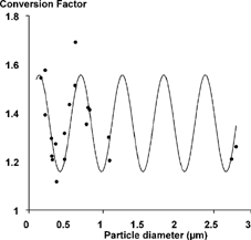
Since the standing wave intensity is (theoretically) a sinusoid of twice the spatial frequency as the laser wavelength, it seemed reasonable to examine the conversion constants in terms of a sinusoidal variation with respect to the ratio d _p /(λ/4), where d _p is the calibration particle diameter and λ is the wavelength. A plot of the individual conversion factors and a fitting function are shown in Figure 1 for the LAS-X.

FIG. 1 Conversion factors for each calibration particle size, together with the fitting function.

The function shown is of the following form:

[3]

and the parameters are given in Table 1. A remains close to the mean value of the set of conversion factors, B allows the conversion factor to vary around the mean value, and C determines the variation rate with particle size. C is reasonably close to ¹/₂ (for which the sine argument would become 2π d _p /λ), but using 0.5 in the fitting function fails to represent the data very well. Using Equation (3) for calibrating the instrument response results in a small, oscillatory bias with a particle size that would probably not be noticed in most calculations. It does seem to be a real phenomenon, however.

TABLE 1 Conversion factors for the LAS-X and HSLAS

Parameter	LAS-X	HSLAS
A	1.36	5.19
B	0.20	0.37
C	0.56	0.56

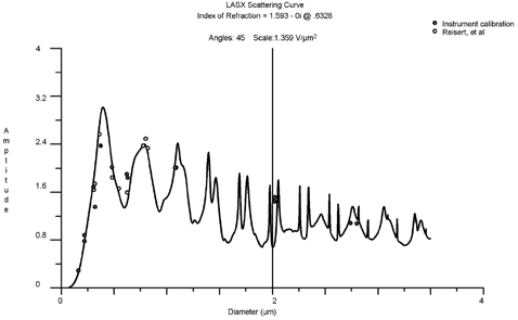
The calculated scattering amplitude for index of refraction 1.593 − 0i is shown in Figure 2. Strictly speaking, the scattering amplitude does not depend on the voltage conversion factor. However, to be able to compare the theory to the experimental data, voltages must be converted to scattering. The data points from Reisert et al. are included in the calibration to show the variation with particle size. Those data are somewhat less certain than the manufacturer's data because the authors did not specify the full-scale voltage for their Multichannel Analyzer (MCA). Using an MCA full-scale value of 3.0 volts produced these results, which seems reasonable.

FIG. 2 Calculated scattering amplitude for PSL as a function of particle diameter using manufacturer's calibration data and measurements of Reisert et al. The points at 2.02 μ m do not affect the scale factor.

Counting Efficiency and Sizing Variations

Having observed effects of the standing wave on the scattered light from calibration particles, we would like to evaluate potential effects on other aspects of particle measurements, particularly counting efficiency and the sizing of particles.

The use of calibration voltages derived from known particles compensates for most of the effects of the standing wave pattern because all particles would see the same patterns on average. There are extreme cases for which the calibration particles do not provide compensation. Consider a very small particle, say, 10 nm in diameter. In the maximum of the laser standing wave, it should scatter close to 10⁻⁶ of the light that a 0.1 μ m particle does, producing about 4 × 10⁻¹⁰ volts with a pulse of light as it passes through the LAS-X beam. However, the same particle on a parallel path only 0.16 μ m away along the beam direction would scatter hardly any light at all because it would pass through a minimum on the standing wave. For small particles, the standing wave pattern is very significant.

Kreisberg et al. (1997) measured the counting efficiency of a LAS-X and found that there was 100% counting of DOS (dioctyl sebacate) particles down to 0.15 μ m, using differential mobility analyzer (DMA) classification and a condensation nucleus counter (CNC) for concentration. For smaller sizes, the counting efficiency dropped rapidly to about 85% at 0.14 μ m and 35% at 0.12 μ m.

We interpret this as a standing wave pattern effect with two contributions. First, particles that passed through various parts of the standing wave experienced different intensities of illumination. Then those particles with less illumination were not counted because the light pulses produced voltage pulses below the minimum counter threshold. There are other factors that do produce loss of particle counts: (1) passing through a lower intensity, off-axis portion of the laser beam; or (2) having a spread in the particle size distribution near the counting threshold. The standing wave pattern affects particles that would always be counted if they passed through a region of maximum beam intensity.

The fact that particles of 0.15 μ m or larger were counted at 100% is significant. A particle of 0.16 μ m is large enough that at least some part of it is illuminated in the standing wave by an intensity of half the maximum value. Normally, DOS of 0.15 μ m diameter would be counted in Channel 2 of the LAS-X (in mode 3). Particles producing slightly less than half the voltage would still be counted, but in Channel 1. However, for only slightly smaller sizes, some particles would produce voltages smaller than acceptable for Channel 1 and would not be counted at all. The fraction of particles producing uncountable pulses grows rapidly as the particle size decreases.

In addition to the loss of particle counts, there is potential for seriously mis-sizing particles up to about 0.32 μ m. As indicated previously, some 0.15 μ m DOS particles would produce pulses of half the maximum amplitude and be counted in the next lower channel. We would like to quantify the error, if possible.

We start with an important assumption about the excitation of the light scattering in a standing wave pattern. The assumption is that the particle scatters light in proportion to the maximum intensity in the standing wave that illuminates any portion of the particle's surface. That is, if any portion of the particle passes through the peak intensity region of the standing wave, the particle will produce scattered waves of maximum amplitude.

Arguments in support of this assumption are as follows: (1) standing wave patterns are the result of waves traveling in opposite directions, each of which would pass through the particle with maximum amplitude; and (2) the particle is essentially a high-Q cavity that is pumped by the incoming waves. The circulating light within the particle will be pumped to the maximum amplitude consistent with the incident waves.

This assumption means that any particle larger than λ/2 will scatter light with the same amplitude, no matter what its trajectory is with regard to the standing wave pattern, because some part of each particle is in a region of maximum intensity. For particles smaller than λ/2, the intensity of the scattered light will be trajectory-dependent. If a particle passes within one radius length of an intensity maximum, then the particle will scatter light with maximum intensity. If the center of the particle passes through the minimum intensity of the standing wave, then the particle will scatter light with intensity determined by the outer boundaries of the particle.

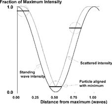
Figure 3 shows a schematic of the relationships between particle trajectories and the standing wave pattern.

FIG. 3 Illustration of the passage of 0.05 μ m particles between intensity maxima of the standing-wave pattern with the resulting scattered light intensity. The curve for scattered intensity corresponds to particles whose centers pass a distance from the standing wave maxima.

At the lowest detectable particle sizes for the instruments (nominally 0.09 μ m for LAS-X and 0.05 μ m for the HSLAS), only particles that scatter light with the maximum intensity will be counted; less intense light pulses will fall below the counting threshold. Assuming the particles are uniformly distributed among the peaks and minima, 0.09 μ m particles would be counted with 29% efficiency and 0.05 μ m particles with 16% efficiency. The same calculation for 0.12 μ m particles gives 38% efficiency, close to the experimental value provided by Kreisberg et al., but such a direct comparison does not take into account the size distribution from the DMA or the amount by which 0.12 μ m particles are above the minimum counting threshold. ²

The conceptual intensity of scattering in the standing wave pattern is captured in the following equations:

[4]

where I is the scattered intensity from the particle, I ₀ is the maximum intensity in the standing wave, d _p is the particle diameter, and λ is the laser wavelength. This means that particles larger than λ/2 scatter light with the maximum intensity.

[5]

where x is the distance from the center of the particle to a standing wave maximum. This means that particles within one radius of a maximum scatter light with maximum intensity. Equations (4) and (5) are equivalent, but express different concepts.

[6]

This means that the cosine-squared dependence applies for values of x greater than one particle radius and less than one particle radius from the minimum. Using Equations (4)–(6), it is feasible to predict the scattering voltage for particles passing through the laser beam at any position relative to the standing wave pattern.

Laser Beam/Particle Beam Interaction

The LAS-X laser operates in the TEM₀₀ mode, which gives the beam a Gaussian intensity cross section (transverse to the standing wave pattern and changing phase with respect to the center of the beam) across the beam profile. The width of the beam is specified as 600 μ m at points corresponding to 1/e ² of intensity (1/e in amplitude). This corresponds to the off-axis intensity being described by a normal distribution with a standard deviation of 150 μ m.

The particles are formed into a beam of sorts at the inlet: particle-laden gas is introduced in the center of a flow of sheath air at a 1:20 ratio in volume flow. The total flow emerges through a small (about 700 μ m) diameter nozzle a few millimeters away from the laser beam. The manufacturer specifies the jet diameter as 500 μ m, which may be due to vena contracta effects in the nozzle. If the particle-carrying core flow remains confined to the central region of the jet, it would occupy 1/21 of the cross-sectional area of the jet, a diameter of 109 μ m in this case. Other volume flow ratios would give other particle beam diameters.

We assume that the particles within the core are uniformly distributed: if the convergence of the particle and the sheath stream is done smoothly, there should be little shear between the two flows and little subsequent mixing. Some of the particles near the outer edge of this core, almost 55 μ m from the center, would pass through the laser beam at a distance of 0.36 (that is, 55/150) standard deviations from its center and experience a relative intensity of 0.937. This 6% loss of intensity is reflected directly in the pulse voltage and means that some of the particles will appear to be smaller than they actually are. This effect does not depend on particle size as the standing wave effect does; it would affect the counting efficency somewhat for particle sizes near the counting threshold.

Is a change of this magnitude detectable in the instrument? In some situations, it is. In an experiment, a mobility classifier was used to calibrate the LAS-X. The electrode voltage (particle size) was adjusted to produce nearly equal counts in two adjacent LAS-X channels; the average calibration particle was therefore on one of the channel boundaries. Changes of mobility (and diameter) of 1% were easily detected in the relative counts between the channels. In practical terms, the laser and particle beam interaction will cause some of the particles near a channel edge to be counted in the next lower channel. This means that the practice of calibrating a channel boundary by splitting the counts equally between adjacent channels is now seen to contain a small inherent error.

This analysis also shows the importance of the diameter of the particle beam for controlling the resolution of the instrument. Makynen et al. (1992) examined the effect of relative sheath air and inlet flows for an instrument similar to the LAS-X and found a decided improvement in resolution when the inlet flow/sheath air flow ratio was reduced. If the ratio is increased, the particle beam will broaden and the voltage pulse distribution will shift noticeably toward smaller particle sizes.

On the other hand, if the center of the particle beam is not perfectly aligned with the center of the laser beam, the spreading effect can be even larger because some of the particles formerly in the center of the laser beam move toward the edges; a greater fraction of the particles will be sized smaller than they are.

We consider it likely that Makynen et al. used a slightly misaligned instrument judging from the way that the pulse height distribution changed with inlet/sheath flow ratio. That is, narrowing the particle beam caused the voltage pulse amplitude distribution to narrow on the high amplitude side, not on the low amplitude side as would be expected if the particle beam were centered on the laser beam. This implies that the LAS-X can be accurately aligned by maximizing the upper side of the pulse amplitude spectrum for a fixed particle size. The alignment is facilitated by using a monodisperse particle with a diameter in the range that gives a monotonic response, that is, less than about 0.35 μ m for PSL.

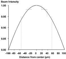
Having identified the shape and standing wave pattern of the laser beam as a source of sizing inaccuracy, how will they be considered in the data inversion? The general solution is that particles of a fixed size will scatter different amounts of light in different zones of the beam. We must treat particles not only by their size, but also by which part of the beam they pass through. For the Gaussian beam shape (which is only a 6% effect at maximum for all particle sizes), we arbitrarily divide the beam into three equal area zones of different incident intensity and then modify the calibration for the three zones, as shown in Figure 4.

FIG. 4 Intersection of the particle beam with the laser intensity profile. The three equal area bands have average intensities of 0.998, 0.982, and 0.950 of the maximum laser beam intensity.

For the standing wave pattern effect, which can be almost an 85% effect at 0.05 μ m, we use equal zones aligned with portions of the standing wave pattern to calculate averages for each particle size.

In most LAS-X data, the correction for laser beam profile is barely noticeable because the channel bins are much wider than the amount of correction. The significance of this effect should be gauged by the importance of small size changes on the overall size distribution. It is also observed that if the instrument has counts in one channel and no counts in the next lower channel, then no particles in the distribution could be right at the common channel boundary size or there would be some spillover.

However, the mis-sizing correction with the standing wave effect can be substantial. At the lower end of the particle size spectrum, 20–40% of particles can register at least one channel lower than they should. In the HSLAS, and in the linear modes of the LAS-X, the low channels are much narrower in size than the broadband LAS-X channels. The mis-sizing can be up to three channels, and large fractions in many of the lowest channels may not be counted at all.

Identifying and quantifying these effects would be a fruitless exercise if there were not some way to recover size distributions after taking them into account. The following sections address the inversion of the counter data to recover size distributions.

Data Inversion Problem

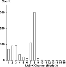
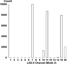
To begin consideration of data inversion, consider a count histogram taken on the LAS-X with a mondisperse PSL aerosol to check its calibration; see Figure 5. The information consists of counts by channel for 15 channels, with the sixteenth channel counting all particles larger than its upper boundary. The manufacturer provides the discriminator voltages corresponding to the channel boundaries and approximate sizes for those boundaries based on calibrations with PSL spheres. The inversion problem is to recover the size distribution that produced these counts and to do so with a size resolution that is compatible with the resolution of the optical response calculations.

FIG. 5 LAS-X counts using a lab-generated PSL aerosol, nominally 0.70 μ m diameter. The nominal boundaries for Channel 8 are 0.5 and 0.65 μ m. Counts in Channels 1–5 are probably due to surfactant in the PSL solution.

Data inversion methods that attempt to improve on the resolution inherent in the data give rise to an infinity of solutions because there are more unknowns than equations. The user of any inversion process must control solutions by applying constraints to produce results that are physically meaningful. Constraints can be internal (“smooth,” “nonnegative”) or external (particles must be between certain size bounds). Often, constraints are implicit in the inversion method, such as fitting to a lognormal distribution; in others, they must be specifically applied. Constraints are always necessary.

We have developed an inversion that mimics the passage of particles through the optical counter: select particle sizes at random; compute their scattering as they pass through the laser beam; and count them in appropriate bins. When the simulated counts match the actual counts, we will have a reconstructed particle size distribution. We call this physically reasonable technique “stochastic reconstruction.” Another form of reconstruction is described in Lawless (2001), which could also be applied to the coarse bin structure of the LAS-X, but does not account for the sensitivity of the response to index of refraction and size parameter and the cross-channel effects.

Stochastic Reconstruction Technique

Stochastic reconstruction simulates the passage of particles through an instrument by generating pseudo-particles at random sizes, computing the instrument response to that size and trajectory, and adding counts to both a high resolution array and a low resolution array that matches the data histogram. When the low resolution histogram exactly matches the measured data, then the high resolution array contains a valid solution for the measurement inversion.

Stochastic reconstruction avoids the multivalued nature of the optical response inversion, because it computes the count in the same way the instrument measures it. Each particle produces a unique pulse amplitude that can be counted in only one channel. This method inherently produces nonnegative size distributions.

Particle sizes are represented by narrow histogram bins covering the normal instrument sizing range. A narrow bin width allows the use of a single value of diameter to represent the optical response accurately. Thus, for the examples we will use, we divide the LAS-X size range, 0.1–3.5 μ m, into 1,200 bins, the first 600 up to 1.0 μ m on a logarithmic scale, the next 600 on a linear scale to the maximum diameter used. There are roughly 75 bins per LAS-X channel. Note that “bin” refers to a size in the reconstructed distribution, while “channel” refers strictly to a set of voltage discriminator settings in the LAS-X.

For each bin diameter, we calculate a scattering voltage curve for the desired index of refraction. Then the scattering voltage for each bin is compared to the discriminator settings to determine in which channel a particle of that size will be counted. Each bin is assigned to a specific channel. Those bin sizes that are too small to scatter detectable light are ignored. When we include the beam and standing wave effects, it will be by changing the amplitude of the voltage pulse produced, not by changing the relationship between voltage and channel.

There is a subtle consideration for adding counts to the inlet bins and output channels. The channel totals should reach the target counts at about the same time, just as the target counts are acquired over a time interval. The reason for this requirement is that cross-channel effects may be influenced adversely if the rate of counting is very different on opposite sides of a channel boundary. We would not expect 0.99 μ m particles to be much less prevalent than 1.01 μ m particles, even if the channel count from 0.9 to 1.0 μ m were one-tenth the count from 1.0 to 1.1 μ m. In a sense, we are asked to constrain the size distribution before we can begin generating it.

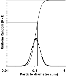
We can accomplish the goal of equal channel counting rates by using the cumulative number distribution to select bins with the random number generator, as shown in Figure 6. This method of generating bins has been chosen for two reasons: it fulfills the channel filling requirement, and it allows the use of a uniform random number generator to select the bins. By filling the channels at roughly the same rate, cross-channel effects will be more accurately simulated. The initial cumulative distribution can be obtained by distributing the measured channel counts equally among the bins that contribute to each channel.

FIG. 6 A uniform deviate between 0 and 1 selects a fraction on the cumulative curve. The diameter bin that corresponds to the fraction is incremented. The resulting histogram resembles the derivative of the cumulative curve, but it has been constructed randomly.

A “reconstruction” consists of picking cumulative fractions with a uniform random number generator (Craig, 1988), incrementing both the bin total and the channel total, and comparing the channel total to the actual channel count. Once the channel total equals the actual channel count, that channel is closed (no more counts are added). When all channels have been closed, the reconstruction is complete. The counts in each bin represent the number of particles of that size that contributed to the channel counts. The total bin histogram represents one valid solution for a size distribution that satisfies the actual channel counts. But this is only the beginning.

The stochastic nature of this method lies not only in the random selection of bins during a reconstruction, but also in the repetition of the reconstruction many times to allow the random fluctuations of the bin count to reinforce or obscure features of the bin size distribution. We assume that by comparing successive reconstructions, we will be able to distinguish features that are persistent, hence, “real,” from those that are transitory.

This could be achieved by simply averaging multiple independent reconstructions. However, we also prefer to introduce a bias toward the reconstructed solution by making successive reconstructions depend on the earlier ones by updating the cumulative distribution from averaged independent reconstructions. This allows the prominent features of the size distribution to reinforce one another, but tends to cancel statistical fluctuations in the cumulative total.

If we apply this technique to the data of Figure 5, we obtain the results in Figures 7–10, which show the 0th approximation and reconstructions for 1, 4, and 20 successive repetitions, with smoothing constraints described below.

FIG. 7 Starting bin approximation for channel count data. The initial bin counts are determined by dividing the channel count data by the number of bins contributing to each channel. The narrow bin count at 0.93 μ m is produced by a small dip, shown in Figure 2 at the same size, that barely drops into Channel 8.

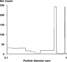
FIG. 8 First stochastic reconstruction of the channel data. The cumulative distribution constructed from Figure 7 was smoothed before these data were generated. This curve is the average of three separate reconstructions using the same cumulative curve. A final smooth was applied to the average.

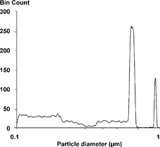
FIG. 9 Fourth stochastic reconstruction of channel data. The cumulative distributions from each prior reconstruction were smoothed. This curve is the average of three separate reconstructions using the latest cumulative curve. A final smooth was applied to the average.

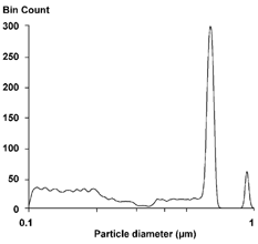
FIG. 10 Twentieth stochastic reconstruction of channel data. The cumulative distributions from each prior reconstruction were smoothed. This curve is the average of three separate reconstructions using the latest cumulative curve. A final smooth was applied to the average. The narrow initial peak at 0.93 μ m has been smoothed away.

Constrained Stochastic Inversion

The raw stochastic inversion technique gives solutions for this problem that are not very satisfactory. We examine methods for constraining the technique to find more physically consistent solutions.

Averaging

Averaging the bin counts from multiple reconstructions will reduce the fluctuations between adjacent bins. However, since the bin totals are always forced to match the channel data, the bin averages simply approach the 0th approximation. There are no mathematical operations involved to couple the solutions that contribute to different data channels.

Smoothing

Our intuitive understanding of particle size distributions requires them to have a degree of smoothness analogous to continuous functions in mathematics. Since stochastic reconstruction itself has no smoothness constraints, we must impose smoothness deliberately to achieve whatever conceptions we have about the size distribution. If we are measuring a monodisperse calibration aerosol, the desire for smoothness should be tempered by the need to keep the size distribution as narrow and accurately placed as possible. If particles are truly polydisperse, heavy smoothing may broaden the size distribution only slightly.

Smoothing can be applied before, during, or after reconstruction. Smoothing applied after reconstruction is mostly cosmetic: it only reduces the fluctuations of the last reconstruction steps. Smoothing during reconstruction is different: it allows the smoothing function to bias the solution while the fluctuations can still affect the resulting distribution. Smoothing before reconstruction is applied to the cumulative distribution, where it influences the generation of the random bin selections. However, even though the cumulative distribution changes the rates at which bin counts accumulate, the bin counts still remain consistent with the channel data.

Smoothing functions can alter the nature of the reconstructed solution somewhat. The distribution can be broadened, narrowed, or shifted toward higher or lower sizes while reducing the count difference between adjacent bins. With histogram data, smoothing functions are often written as multipoint algorithms that are applied repeatedly over the bin range.

The optical response curves and reconstruction bins can easily consist of several thousand points, as needed to reveal optical resonances. Multipoint algorithms must span large numbers of points or be applied repeatedly to show an influence in the computed size distributions. We have found that a simple running average passed across the computed size distribution once or twice is adequate if the average spans 0.5–2% of the total number of bins. The formula used is the following:

[7]

where i is the index of the point being averaged and m is the number of points being averaged in either direction. When the running average approaches the end of bins at either end of the size distribution, the averaging bounds are truncated appropriately to avoid bringing zeroes into the average. Tailoring of the contributions at the end of the averaging interval can be applied to reduce the impacts of sudden changes in bin counts as the average interval passes into a high count region.

The finer details of the averaging process make little difference in the final size distributions because the feedback through the cumulative distribution to the next round of reconstruction makes the process converge nicely.

Convergence

Since each reconstruction is consistent with the original data, the only criteria for method convergence are those associated with smoothness. These can take the form of maximum (or average) change between bin counts from one cycle to the next or maximum (or average) change between adjacent bins at the end of a cycle of reconstructions. Whatever criterion is chosen, eventually the change in the criterion will be driven by the randomness in each reconstruction, forming a “noise” floor against further improvement in smoothing.

Too much smoothing or too many cycles may eliminate features that could be “real.” The narrow peak at 0.93 μ m in Figures 7–10 doesn't seem likely to be real, standing apart from the rest of the size distribution as it does. Other disappearing peaks might not be so clear.

Accommodating Standing-Wave and Beam Effects

The voltage response curve calculated from Equations (1) and (3) represents the highest voltage pulse that can be produced by a particle passing through the laser beam axis through a standing wave maximum. Passing through any other beam position will produce a pulse that is smaller in amplitude. If we limit the computations to a few positions with equal probabilities, then the application of the stochastic reconstruction can include those position effects with minor increases in complexity.

We have implemented a five-position standing-wave average, computing the average amplitude for five equal zones from the maximum to the minimum. When these five zones are combined with the three beam-axis averages (Figure 4), there are 15 equally likely voltage responses that one particle can produce passing through the beam. By designing the zones with equal areas, it is feasible to cycle through all 15 zones, selecting only the particle size at random and picking a bin according to the curve that corresponds to the zone that is current. In this way, a particle can contribute one count to a channel that is lower than the ideal voltage curve would select.

In the case of particles near the lowest channel boundary, some particles might not be able to contribute a count, even though they are of a size that would count if the position in the beam were in a higher amplitude zone. Some careful accounting allows these particles to accumulate in the proper size bin, so that more particles are predicted than are actually counted. This is roughly equivalent to dividing the actual counts by the counting efficiency to obtain an estimate of the true particle concentration.

These effects show the need for care in generating the random numbers. It would be possible, for example, to satisfy a channel count with improperly-sized large particles before any properly-sized smaller particles could contribute, if the order of accumulation were not properly randomized.

As a check on the method, artificial LAS-X data was generated, consisting of 30,000 counts in one channel only for all 16 different channels. The peak of the resulting reconstructed size distribution was recorded five times. Table 2 gives the statistics for one set of smoothing parameters (1% of the bins) and convergence criterion.

TABLE 2 Results of fitting single channel data using 1.593 + 0i

	#						Relative
	Initial	Total	Peak	FWHM	Mean peak	Standard	standard
Channel	peaks	count	(μ m)	(μ m)	count	deviation	deviation
1	1	36800	0.113	0.019	894	1.5	0.002
2	1	30000	0.146	0.020	884	2.2	0.002
3	1	30000	0.185	0.031	773	2.0	0.003
4	1	30000	0.229	0.031	882	2.9	0.003
5	1	30000	0.272	0.034	950	1.6	0.002
6	1	30000	0.326	0.053	751	1.6	0.002
7	1	30000	0.447	0.215	286	2.5	0.009
8	2	30000	0.639	0.057	1249	0.5	0.000
9	3	30000	0.707	0.345	513	1.4	0.003
10	4	30000	1.565	0.108	581	3.7	0.006
11	6	30000	1.140	0.121	679	1.5	0.002
12	3	30000	2.110	0.087	870	3.7	0.004
13	4	30000	2.223	0.463	523	4.1	0.008
14	5	30000	3.235	0.117	682	5.0	0.007
15	10	30000	2.935	0.196	646	3.6	0.006
16	6	30000	3.435	0.154	592	2.8	0.005

The single data channel produces as many as 10 distinct initial bin groups at the higher channel numbers. Smoothing often reduces the peaks to only one or two. The total count reproduces the channel data exactly, except for Channel 1, where 23% of uncounted particles added to the total. The particle size corresponding to the peak count is shown, as well as the full width at half maximum. In Channel 7, the FWHM is large because the peak is very broad; in Channels 9 and 13, the FWHM spans at least two distinct peaks of nearly equal height. The Channel 14 peak occurs at a larger size than the Channel 15 peak because one of the largest size multiple peaks became dominant during the reconstruction.

The peak counts differ because the channel widths vary across the size spectrum. The peak count and the bin number of the peak do exhibit slight variation from one reconstruction to the next, but the overall variation is agreeably small. The reconstruction algorithm is quite reproducible, as demonstrated by these results. It should be noted that measurement of 30,000 particles would be expected to have a standard deviation of 173 particles, a Relative Standard Deviation (RSD) of 0.006. We therefore assert that the reconstruction process will not introduce much more imprecision in the count or concentration than is already inherent.

The unrealistic nature of the collapse of several narrow peaks into a single narrow peak is a result of the inversion problem itself: the smoothness constraint was not sufficient to produce a realistic size distribution. (But, too, how realistic is a single channel with counts?) A stronger smoothing constraint can force all the multiple peaks to coalesce into one. Likewise, having data in adjacent channels can improve the realism of the reconstruction.

The optical effects that have been addressed dictate that it is impossible to accurately reconstruct a single data channel in the lower channels of the HSLAS or in Mode 2 of the LAS-X. Real monodisperse particles will be counted in more than one channel. Likewise, above 1 μm in diameter, reasonably narrow particle distributions will produce counts in several adjacent channels as the optical resonances are encountered. For example, PSL particles near 2.0 μ m with a 1% spread could contribute to counts in four channels in the LAS-X.

SIMULATED MONODISPERSE MIXTURES

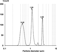
Single channel data is readily constructed by hand. To simulate real particles being counted, the laser response curve can be used with a numerical particle generator to accumulate counts in the proper LAS-X channels. Since monodisperse PSL particles are available with standard deviations of 1–2% of the nominal size, normal distributions were used to construct a composite data set. Mean diameters were 0.481, 1.09, and 2.8 μ m, chosen to correspond to calibration data points. Ten thousand particles of each diameter, chosen at random from a normal distribution of standard deviation of 1%, were accumulated into LAS-X channels. The resulting channel histogram is shown in Figure 11.

FIG. 11 Synthesized channel data from 10,000 “particles” each at 0.48, 1.09, and 2.8 μ m.

Although all the particles at 0.48 μ m were accumulated in Channel 7, any size between 0.38 and 0.56 μ m would also have been accumulated solely in Channel 7 due to its width. At the other diameters, changes of 0.01 μ m were easily discerned in the counts. This data was then reconstructed using a 2% smooth, with the results shown in Figure 12.

FIG. 12 Reconstruction of synthesized channel data from Figure 11. The triangles indicate the diameters that generated the data in Figure 11.

The reconstruction cleanly separates the major peaks, while leaving some small artifacts. The reconstructed peak at 0.48 would have been the same for any input particle between 0.38–0.56 μ m, but that is solely due to the response curve. The differences at the other challenge sizes are also due to the multivalued response curve, but there is sufficient additional information in Channels 10, 14, and 16 in the data set to focus the reconstruction quite closely near the input values. Some narrowing of the 1.09 and 2.8 μ m peaks could be obtained by using a narrower smoothing function, but the differences are not large.

It is interesting to note the small peak at about 1.90 μ m. If the LAS-X is challenged with a distribution centered at 1.90 μ m, a small fraction of the counts accumulate in Channel 12. However, in the Figure 11 data, there are no counts in Channel 12, and therefore the reconstruction slowly eliminates any particles from that region as inconsistent with the response curve. If a small number of counts had been added to Channel 12, the peak would persist and contain only the Channel 12 counts.

RESULTS FOR TITANIUM DIOXIDE

The final problem is the application of these methods to the titanium dioxide sizing measurement. Figure 13 shows the raw LAS-X distribution obtained for TiO₂, taken by aerosol sampling and dilution from a pigment finishing line (Lawless, 1992). The pigment is composed of primary spherical particles of about 0.2 μ m diameter, most of which are sintered into dense aggregates of about 0.5 μ m diameter; any particles larger than about 0.6 μ m are likely to be less dense aggregates, based upon electron micrographs. Using Equation (2), we have calculated the scattering voltage curves for one index of refraction (2.652, 0i), as shown in Figure 14. Since TiO₂ is birefringent and the particles are not spherical over the whole range, Mie scattering is not strictly applicable, but, for now, we will use this curve and assume spherical particles.

FIG. 13 Counts obtained by dilution for titanium dioxide pigment from a production line.

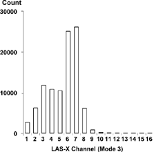
FIG. 14 Calculated LAS-X voltage response to spherical TiO₂ particles with index of refraction 2.652 − 0i. The individual curves for the interference calculations are shown below 0.3 μ m. The horizontal lines define the channel voltage thresholds.

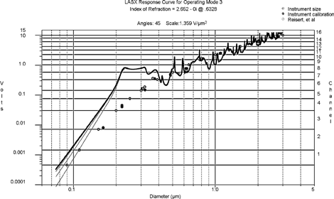
The broad, flat region of the curve between 0.2 μ m and 0.4 μ m is one of the problem areas for using the LAS-X with titanium dioxide. It is impossible to determine a unique size from the pulse heights for particles in this range.

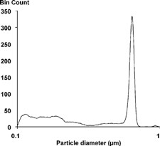
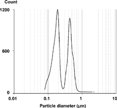
The reconstructed size distribution is shown in Figure 15. The relevant features are the two peaks at 0.19 μ m and 0.42 μ m, with relatively few particles in the 0.2–0.4 μ m region. The first peak is assumed to be primary particles and the second well-sintered aggregates. Other, smaller peaks appeared on the shoulders of the 0.4 μ m peak, but were smoothed away in the reconstruction by using a somewhat broader smoothing function.

We find it difficult to say that these minor peaks are real features of the size distribution without some confirming evidence. The assumptions that the particles are spherical and isotropic are stringent in generating the response curves, but the two main peaks do not change their positions or relative sizes very much when using the higher index of refraction for titanium dioxide, 2.952 − 0i, nor for a blend of the two indices of refraction. Even adding an absorptive component, 2.652 − 0.02i, which smooths the response curve noticeably, does not affect the main peaks. The smaller peaks are more strongly affected.

It has been asked whether a more judicious choice of channel thresholds would be advantageous; the answer is not completely clear. More channels below 0.2 volts (corresponding to 0.2 μ m) would afford increased resolution near the lower peak, but those are the channels most strongly affected by the standing wave effect, with the strongest cross-channel counting. In the region near the first resonance, Channels 6–8, some adjustment of thresholds would confine the Channel 6 response to sizes near 0.2 μ m, give Channel 7 a relatively narrow size region at 0.4–0.5 μ m, and broaden the Channel 8 response to include more particles near 0.5 and 0.6 μ m. This modification might improve the solution resolution in this region. Above Channel 8, very little will be gained by trying to optimize channel thresholds, in the sense of improving resolution. The mixing of responses from particles widely separated in size means that the choice of smoothing parameter will affect the solution much more than shifting a small fraction of counts from one channel to another.

FIG. 15 Reconstructed TiO₂ size distribution, using a 2% smoothing parameter.

SUMMARY

The laser-based instruments, LAS-X, HSLAS, and the like, appear to have a very calculable voltage response. Some small effects have been noted in the variation of conversions factors for various sizes of calibration particles, while others were inferred from beam geometries and counting efficiency measurements. Although these effects are relatively minor, the fact that they can be observed and, to a large extent, predicted accurately means that the theoretical response is well understood and can be usefully applied to other types of particles.

Stochastic reconstruction was devised as a means for using the complex optical response of these instruments to recover realistic size distributions and extend their usefulness. It cannot recover more information than is in the original data, but it can select realistic possibilities from an infinity of solutions.

Stochastic reconstruction is a flexible tool because its use can be tailored in many ways. It is designed to obtain solutions where the function to be inverted is fine-grained and multivalued. By design, its solutions are nonnegative. The reconstructions that have been used as illustrations show differences with the choice of fitting parameters, but numerous tests have also shown that the method is robust.

These properties are not without cost. The computer program requires tens of seconds on a 400 MHz PC for the reconstructions. This is fast enough to keep up with real-time data acquisition, but slow enough to make processing of archived data tedious. The combinations of parameters available to the user make insightful choices necessary, least time be wasted in generating reconstructions that have no meaning.

The combination of the calculable response of the LAS-X and an analysis method that can make use of the response is very powerful. Other types of laser counters whose geometries are known should be able to be calculated in the same manner, whether the laser beam is unidirectional or bidirectional, using Equation (1). Even “white light” counter responses can be calculated with some weighting of response curves according to the combined wavelength dependences of the source and detector.

Real aerosols do pose additional problems that we have barely addressed (the birefringent nature of TiO₂, for one). There is a body of work that suggests that Mie theory is not too much in error for shapes that are almost spherical, particularly in the forward direction (Bohren and Huffman, p. 311 ff., p. 427 ff.; also, Gebhart, 1991) so it is possible to use approximate indices of refraction to predict the instrument response. Particles in the accumulation mode are unlikely to have the same indices of refraction as particles in the coarse mode, so some joining of response curves would be necessary to apply the reconstruction method as written. Using DMA-classified aerosols in narrow size ranges with one of these counters, it is possible to estimate, if not completely determine, the particles' index of refraction.

CONCLUSIONS

The laser-based particle sizing spectrometer has become a widely used instrument without a firm theoretical basis for its calibration. The experimental and theoretical efforts of others have established that Mie theory can be applied to calculate the response of such spectrometers for spherical particles. However, outside a limited range of index of refraction, the discrimination of the instrument for particles of different sizes is limited by broad size band limits and nonmonotonic light scattering.

By using stochastic reconstruction, many problems of recovering the size distribution can be eliminated. In particular, the inversion of nonmonotonic scattering voltage curves is no longer difficult. Stochastic reconstruction is a robust technique in the sense that changes in the details of smoothing do not alter the recovered size distribution very much. The size distribution does depend on the assumptions that the user asserts, such as the initial bin counts and smoothing functions. Stochastic reconstruction should be considered a data analysis tool, one that opens certain difficult problems to solution. Like any tool, it can be misused or misapplied. The laser spectrometer is a good application for the tool.

Acknowledgments

This paper was originally accepted for publication in 1991, but extensive revisions were requested and could not be made until recently. In the meantime, co-author Seb Mastrangelo retired from duPont and, several years later, passed away. Without his influence and guidance, we would never have addressed the difficult problem of sizing titanium dioxide pigments with an optical counter.

Notes

¹Calibration with 2.02 μ m PSL gives strange results, because the nominal diameter falls almost exactly between two narrow scattering peaks in the computed correlated scattering. Minor changes in diameter would produce large changes in voltage. Accounting for the normal Gaussian standard deviation of the particles, scattering from both peaks is expected. We do not use the 2.02 μ m particles in the calibration.

² Subsequent computer evaluations using the factors developed in this article gave counting efficiencies for DOS of 82% at 0.14 μ m mean diameter and 38% at 0.12 μ m, using a triangular size distribution of the type a DMA produces. All particles counted in LAS-X Channel 1.

REFERENCES

- Bohren , C. F. and Huffman , D. R. 1983 . Absorption and Scattering of Light by Small Particles , New York : Wiley .
- Chen , B. T. , Cheng , Y. S. and Yeh , H. C. 1984 . Experimental Responses of Two Optical Particle Counters . J. Aerosol Sci. , 15 : 457 – 464 .
- Craig , J. C. 1988 . The Microsoft QuickBASIC Programmer's Toolbox , Redmond, WA : Microsoft Press .
- Garvey , D. M. and Pinnick , R. G. 1983 . Response Characteristics of the Particle Measuring Systems Active Scattering Aerosol Spectrometer Probe (ASASP-X) . Aerosol Sci. Technol. , 2 : 477 – 488 .
- Gebhart , J. 1991 . Response of Single-Particle Optical Counters to Particles of Irregular Shape . Part. Part. Sys. Charact. , 8 : 40 – 47 .
- Hinds , W. C. and Kraske , G. 1986 . Performance of PMS Model LAS-X Optical Particle Counter . J. Aerosol Sci. , 17 : 67 – 72 .
- Knollenberg , R. G. 1979 . “ Single Particle Light Scattering Spectrometers ” . In Aerosol Measurement , Edited by: Lundgren , D. A. , Harris , F. S. Jr. , Marlow , W. H. , Lippmann , M. , Clark , W. E. and Durham , M. D. pp. 271 – 293 . Gainesville, FL : University Presses of Florida .
- Kreisberg , N. , Stolzenburg , M. and Hering , S. 1997 . Ambient Calibration of an LAS-X Optical Particle Counter , Research Triangle Park, NC : Research Triangle Institute . Final Report, Contract No. 1–93N-6786
- Lawless , P. A. 1992 . U.S. Patent No. 5,109,708 . Sampling System and Method for Sampling Concentrated Aerosols ,
- Lawless , P. A. 2001 . High Resolution Reconstruction Method for Presenting and Manipulating Particle Histogram Data . Aerosol Sci. Technol. , 34 : 528 – 534 .
- Makynen , J. , Hakulinen , J. , Kivisto , T. and Lehtimaki , M. 1982 . Optical Particle Counters: Response, Resolution and Counting Efficiency . J. Aerosol Sci. , 13 : 529 – 535 .
- Reisert , W. , Roth , C. , Gebhart , J. , Fischer , P. and Schafer , R. J. 1991 . Intercavity Laser Light Scattering: Experimental Verification of Theoretical Response Functions . J. Aerosol Sci. , 22 : S355 – S358 .
- Soderholm , S. C. and Saltzman , G. C. 1984 . “ Laser Spectrometer: Theory and Practice ” . In Proc. First International Aerosol Conference , Edited by: Liu , B. Y. H. , Pui , D. Y. H. and Fissan , H. J. pp. 11 – 14 . New York : Elsevier .
- Szymanski , W. W. and Liu , B. Y. H. 1986 . On the Sizing Accuracy of Laser Optical Particle Counters . Part. Charact. , 3 : 1 – 7 .