Inverse Modeling of Aerosol Dynamics Using Adjoints: Theoretical and Numerical Considerations

In this paper we develop the algorithmic tools needed for inverse modeling of aerosol dynamics. Continuous and discrete adjoints of the aerosol dynamic equation are derived, as well as sensitivity coefficients with respect to the coagulation kernel, the growth rate, and the emission and deposition coefficients. Numerical tests performed in the twin experiment framework for a single component model problem show that the initial distributions and the dynamic parameters can be recovered from time series of observations of particle size distributions.

INTRODUCTION

As our fundamental understanding of atmospheric particles and their transformations advances, novel computational tools are needed to integrate observational data and models together to provide the best, physically consistent estimate of the evolving state of the atmosphere. Such an analysis state better defines the spatial and temporal fields of key gas and particle phase chemical components in relation to their sources and sinks. This information is critical in designing cost-effective emission control strategies for improved air quality, for the interpretation of observational data such as those obtained during intensive field campaigns, and to the execution of air-quality forecasting. The development of the tools to integrate measurements and models is also critical to the challenge of a full utilization of the vast amounts of satellite data in the troposphere that are now becoming available, and which will become more prevalent in the coming years.

Assimilation of chemical information is only now beginning in air quality/chemistry arenas (Elbern et al. 1997; Sandu et al. 2003; Daescu et al. 2003; Sandu et al. 2004; Sandu et al. 2005), but offers the same motivations as those realized in the field of meteorology. Assimilation techniques can be utilized to produce three-dimensional, time varying optimal representations of the particle distributions in the atmosphere, that are consistent with the observed physical and chemical states.

Forward modeling of aerosols predicts the evolution of particle size distributions given the known parameters of the evolution (coagulation kernel, growth rate, emission rates, and deposition velocities) as well as the initial size distribution. Numerous numerical methods have been proposed in the literature for solving particle dynamics, and several are surveyed in Zhang et al. (1999). Methods for solving coagulation include the semi-implicit scheme (Jacobson 1999), Newton-Cotes quadrature (Sandu 2002), Galerkin (Pilinis 1990; Sandu and Borden 2003), and spline orthogonal collocation (Gelbard and Seinfeld 1978). Methods for solving the growth equation include the moving sectional approach (Kim and Seinfeld 1990; Lurmann et al. 1997; Jacobson 1997), finite volumes (Bott 1989), finite elements (Tsang and Hippe 1988; Meng et al. 1998), quintic splines (Nguyen and Dabdub 2001), semi-Lagrangian methods (Nguyen and Dabdub 2002), and other (Binkowski and Shankar 1995).

The inverse modeling problem consists of recovering the initial or emitted size distribution and the parameters of evolution given information about the time evolution of the system, for example periodic measurements of the number, surface, mass, or volume density. We take the variational approach, in which the inverse modeling problem is formulated as an optimization problem. In this paper the concept of “inverse modeling” is different than inverse in time simulation.

In this paper we develop the algorithmic tools needed for inverse modeling of particle dynamics. Continuous and discrete adjoints of the particle dynamic equation are derived, as well as sensitivity coefficients with respect to the coagulation kernel, the growth rate, and emission and deposition coefficients. For the derivations we consider spatially independent (box) models and focus only on the physical particle dynamics aspects, that is, we do not treat chemical and thermodynamic transformations. We discussed inverse modeling of chemical kinetics in (Sandu et al. 2003), and data assimilation in 3D chemical–transport models (Sandu et al. 2004; Sandu et al. 2005). We have previously analyzed the adjoint equations for aerosols undergoing ideal thermodynamically driven condensational growth in (Henze et al. 2004), and more research is in progress to extend this work to nonideal systems. The methods developed here are a first step toward the goal of performing data assimilation for comprehensive three-dimensional particle chemistry and transport models.

The paper is organized as follows. An overview of the particle dynamics equations and of the forward modeling problem is given in Section The inverse modeling problem is formulated in Section Continuous adjoints are discussed in Section and discrete adjoints in Section A comprehensive set of numerical results on the coagulation and growth equation is presented in Section Section 6, and conclusions are drawn in Section Complete derivations of several continuous and discrete adjoint equations are given in Appendices A. through D.

AEROSOL DYNAMICS

To accurately study the effects of aerosols it is necessary to resolve aerosol number and mass distributions as a function of chemical composition and size. Three major approaches are used to represent the size distribution of aerosols: continuous, discrete and parameterized. In this paper we focus on continuous models (i.e., continuous size distributions and the general dynamic equations in continuous form) with particle size distributions being functions of particle mass (m) and time (t). The formulation follows mainly (Seinfeld and Pandis 1997). We also consider numerical discretizations of continuous models using the piecewise polynomial approach proposed by Sandu (Sandu 2004). The discussion in this paper focuses on physical transformations (growth, coagulation, sources, and sinks) and does not cover chemical transformations.

Number Density Formulation

We first consider the particle dynamic equation in number density formulation, with particle mass the independent variable. The size distribution function (number density) of a family of particles will be denoted by n(m,t); the number of particles per unit volume of air with the mass between m and m+dm is n(m,t) dm. This describes completely a population of single-component particles. The aerosol population undergoes physical and chemical transformations (Seinfeld and Pandis 1997) which change the number density in time:

with the initial and boundary conditions

In this equation I(m,t) = dm/dt is the rate of particle growth (e.g., due to condensation, evaporation, deposition and sublimation), β(m,m′) is the coagulation kernel, S(m,t) is any source of particles of mass m (e.g., nucleation and emissions) and L(m,t) is the first-order rate of removal of particles of mass m (e.g., by deposition).

Mass Density Formulation

We consider now particles composed of multiple chemical constituents i = 1,2,…,r. The total mass of a particle is the sum of masses of its r individual components

To describe the multicomponent population of particles one models the mass concentration distribution of each species i

with the total particle mass concentration distribution being

The total mass density of component i in particles with masses between m and m+dm is q _i (m,t) dm.

The growth (condensation/evaporation) rate of species i is I _i = dm _i /dt. It is customary to use the normalized growth rates

The total growth rate of particles of mass m is

The particle dynamic equation governs the evolution of the mass concentration distribution of each component i = 1,2,…,r (Seinfeld and Pandis 1997).

where m _i S(m,t) is the source term and and L(m,t)q _i (m,t) is the removal term (μ g iμg⁻¹cm⁻³ s⁻¹).

The initial and boundary conditions are

The boundary condition at m = ∞ expresses the fact that there cannot be arbitrarily large particles (e.g., due to removal processes).

Discrete Formulation

In this section we exemplify the derivation of discrete particle dynamics models based on the number formulation of the dynamic equation (1) discretized in size with a piecewise polynomial approach as described by Sandu (2004). A completely similar approach for the mass density formulation is possible.

The finite dimensional approximation of the number distribution n(m,t) is taken in the space spanned by the set {φ _i }_{1 ≤ i ≤ s} of piecewise polynomial basis functions. The dynamic equation discretized in size reads

with the initial condition by projecting the continuous initial condition of (1) onto the finite dimensional space:

The growth terms are discretized using a Discontinuous Galerkin approach where F(n(t)) is the Godunov flux difference and

The coagulation terms are discretized using a collocation approach with collocation points {c _j }_{1 ≤ i ≤ s} . We have

and

A fully discrete particle dynamic equation is obtained by applying a time stepping algorithm to (3). For example the Forward Euler time discretization leads to

where the numerical solution is n ^k ≈ n(t ^k ).

The Forward Modeling Problem

In forward modeling one starts with a known initial distribution, n ⁰(m) or q _i ⁰(m), given boundary conditions and model parameters, I(m,t) or H _i (m,t), β(m,m′), S(m,t), and L(m,t). The evolution of the solution in time is completely described by the particle dynamic equation (1) or (2). In practice a numerical approximation, or discrete model of the form (4), is implemented and approximations of the distribution are computed at discrete time moments.

THE INVERSE MODELING PROBLEM

Variational methods provide an optimal control approach to the data assimilation problem. Four-dimensional variational (4D-Var) data assimilation allows the optimal combination of three sources of information: an a priori (“background”) estimate of the state of the atmosphere; knowledge about the physical and chemical processes that govern the evolution of pollutant fields, as captured in the model; and observations of some of the state variables. The optimal analysis state is obtained through a minimization process to provide the best fit to the background estimate and to all observational data available in the assimilation window.

To be specific, consider the model (1) which describes the evolution of the number density of a particle population given the initial distribution n ⁰(m) and the parameters p of the problem (I(m,t) or H _i (m,t), β(m,m′), S(m,t), and L(m,t)). This equation is called the forward model and describes the (forward in time) evolution of particle density. The general inverse modeling problem consists of finding the initial distribution and the parameter values which minimize an integral cost functional

The functional depends on the initial distribution and the parameter values implicitly, through the mapping of (n ⁰,p) to n(m,t) provided by the forward model. The minimization procedure needs the functional value and its gradients with respect to the model parameters ∇ _{n ⁰} and ∇ _p . For given values of (n ⁰,p) the functional value is obtained by a forward integration of the forward model, while the derivatives can be efficiently obtained through adjoint modeling, as will be explained in the following section.

Data Assimilation

Of particular interest in this paper is the data assimilation problem, where the observations y ¹… y ^N are available at the discrete times t ¹… t ^N . The observed quantities are functions of the solution

Observations can be particle number or mass densities, optical properties, and so on. Data assimilation uses the information from observations to estimate the values of a finite set of parameters p (which can provide a parameterization of the initial solution n ⁰, or determine the forward model parameters I or H, β, S, and L). The cost functional is defined to measure the mismatch between model predictions and observations

The first term penalizes the departure of the parameters from the apriori estimate p _B , and is called the background term. The matrix B is the error covariance associated with background terms and R _k are error covariances associated with observations. The parameters p, which initially have values p _B , are adjusted such that the value of the functional is minimized.

CONTINUOUS ADJOINTS OF THE DYNAMIC EQUATION

In this section we define the adjoint equations for the model (1) that offer a computationally efficient approach to computing the gradients of the cost functional (5) with respect to the model parameters and initial conditions. Note that the functional depends on n ⁰ and p implicitly, since the forward model evolution uniquely determines {n ^k } _{k ≥ 1} from n ⁰ and p. In the continuous formulation one derives the adjoint of the original (continuous in time and size) dynamic equation, to obtain the derivative of the exact solution. For a computer implementation both the forward and the adjoint model are solved using the numerical methods of choice.

Number Density Formulation

The adjoint equation of the tangent linear model of equation (1) for the cost functional (5) defines the evolution of adjoint variables

with the following boundary and initial conditions

A complete derivation of the adjoint equations and the sensitivity relations is given in Appendix A.

The adjoint variables are initialized at the final time T. Equation (7) is defined such that, when integrated backwards in time from T to t ⁰, the value of the adjoint variable at t ⁰ is the sensitivity of the cost functional with respect to initial values λ(m,t ⁰ = ∇ _{n ⁰} . Thus the adjoint Equation (7) provides a method to obtain the gradients needed in the minimization of (5).

The Equation (7) depends on the state of the forward model n(m,t). Consequently, one needs first to integrate the forward model (1) and save the state at all times, then use this information during the backward integration of (7).

The sensitivities of the cost functional (5) with respect to forward model parameters are (see Appendix A):

All the sensitivity coefficients (8a, 8b, 8c, 8d, 8e) of the cost functional can be obtained by one forward in time integration of the forward model (1), followed by a single backwards in time integration of the adjoint model (7). When solving the data assimilation problem each iteration for the minimization of the cost functional (5) requires one evaluation of the cost functional and one evaluation of its gradient, therefore we have one forward and one backward integration per optimization step.

Data Assimilation

For data assimilation the functional (6) is defined at discrete time moments and uses a discrete set of observations. Formally, the function J ₀ in (6) and the corresponding forcing term in (7) contain delta functions at measurement times t ^k . For an equivalent formulation consider t ^k ₋ and t ^k ₊ to be the moments immediately before and immediately after t ^k . The adjoint model (7) is defined on each subinterval [t ^k−1,t ^k ] for k = N,N−1… 1 as

Note that instead of delta forcing terms in this formulation we have explicit jumps of the adjoint variable between intervals (across the observation times). The derivative of p with respect to n may be nonzero for parameters used to define the initial distribution.

Mass Density Formulation

For multiple components the cost functional is defined as

A complete derivation of the adjoint equation and sensitivity coefficients for the multicomponent, mass density formulation (2) is given in Appendix B. The adjoint equation is:

with the initial and boundary conditions:

For data assimilation the adjoint equation can be redefined similar to (9). The sensitivity equations are:

The minimization procedure employed for data assimilation requires at each step one evaluation of the cost functional (10) and one evaluation of its gradient (11a, 11b, 11c, 11d, 11e). Therefore each optimization step is completed using one forward in time integration of the forward model (2), followed by a single backwards in time integration of the adjoint model (11).

DISCRETE ADJOINTS OF THE DYNAMICS EQUATION

In the discrete approach the numerical discretization (4) of the the particle dynamic equation is considered to be the forward model. This is a pragmatic view, as only the numerical model is in fact available for analysis. The adjoint of the discrete model (4) is formulated and solved. The approach amounts to computing the derivatives of the numerical solution, rather than approximating the derivatives of the exact solution. In this section we exemplify the derivation of discrete adjoint techniques based on the number formulation of the dynamic equation discretized with a piecewise polynomial approch (Sandu 2004) and the Forward Euler method (4).

Direct Approach

Taking the adjoint of the discrete equation (4) leads to a method to propagate the adjoint variables backwards in time. The general derivation of the discrete adjoints, including the case of a higher-order explicit Runge Kutta time stepping, is presented in Appendix C. The cost functional is defined in terms of the discrete model state at times t ^j , usually multiples of the integration time step

The adjoint equation of (4) reads

The factor δ^obs _k is one if t ^k is a time point used in the definition of J, and zero otherwise. The adjoint variable at t ⁰ gives the gradient of the cost functional (12) with respect to the initial distribution,

Note that this is the derivative of the numerical solution as used in the definition of (12), as opposed to the continuous adjoint formulation (8a), where λ⁰ defines the derivative of the continuous solution.

In practice the continuous forward model (1) is solved numerically, and so is the continuous adjoint Equation (7). Therefore the continuous adjoint approach is in practice a hybrid approach. The operations of numerical discretization and adjoint do not commute in general, and consequently the numerical solution of (7) is different from the discrete adjoint (13). For data assimilation problems one needs the derivative of the numerical solution, that is, the discrete adjoints are in principle preferred. For sensitivity studies using the adjoint method one wants to approximate the sensitivities of the continuous model, and the continuous adjoint seems more appropriate.

Automatic Differentiation

Given a program that implements the forward model, automatic differentiation builds a new, augmented program, which computes the analytical derivatives along with the original program (Corliss et al. 2001; Griewank 2000). The derivatives are propagated using the chain rule and are accurate up to machine precision. Automatic differentiation can work in forward mode, in which case the tangent linear model is produced, and in reverse mode, in which case the discrete adjoint is produced. Several automatic differentiation tools are available including TAMC (Giering 1997; Giering and Kaminski 1998; Giering), Tapenade (Courty 2003), Adifor, ADOL-C, NAGWare Fortran 95, and so on.

Automatic differentiation has several highly attractive features. First, it requires only (an implementation of) the original forward model. The transformations needed to obtain the adjoint gradients are done completely automatically. This allows, in principle, to perform inverse modeling with any forward model, no matter how complicated. Moreover, parts of the model may be legacy code for which we do not have all the underlying details, and an analytical (continuous) adjoint of this submodels may be impossible to derive. Next, automatic differentiation produces discrete adjoints, therefore derivatives of the numerical solution, which are appropriate for optimization purposes.

In this paper we use the automatic differentiation tool TAMC (Giering 1997; Giering and Kaminski 1998) to generate the discrete adjoint derivatives.

The Role of Forward Numerical Method

Clearly, the formulation of the discrete adjoint equation depends not only on the particle dynamic equation itself, but also on the numerical method used to solve it (to define the discrete forward model). To illustrate the dependence of the discrete adjoint equation on the numerical method used to solve the forward problem we derive in Appendix D the discrete adjoint of the popular semi-implicit method (Jacobson 1999) for solving coagulation. One can compare the coagulation terms in (13) with the discrete coagulation adjoint (D.5). The adjoint derivation (D.5) is useful in its own right for performing data assimilation when coagulation is solved with the semi-implicit method.

NUMERICAL RESULTS

The Test Problem

For the numerical experiments we consider the test problem of aerosol coagulation and growth from (Gelbard and Seinfeld 1978), which admits an analytical solution. Let N _t be the total initial number of particles and V _m the mean initial volume. The initial number distribution is exponential, the coagulation rate is constant, and the growth rate is linear with the particle volume:

The analytical solution in (Gelbard and Seinfeld 1978) is

We solve the dynamic equation for β _o = 2.166 × 10⁻⁶ cm³ h⁻¹ particles⁻¹, σ _o = 0.02 hour⁻¹, N _t = 10⁴ particles, V _m = 0.03 μm³. The value of β _o follows from (Jacobson 1999), and the value of σ _o is chosen such that coagulation and growth have effects of comparable magnitude. The size range is truncated to the volume interval V _min = 10⁻³μ m³, V _max = 1 μ m ³. A piecewise linear discretization with 8 bins is employed for particle size as described in Section 5. Bin centers are log-uniformly distributed in the range [V _min,V _max]. The time interval under consideration is [t ₀ = 0, T = 48] h. The time discretization is performed with the second order Runge Kutta scheme (C.1) with the time step Δ t = 6 min. The actual implementation is done in the (equivalent) volume concentration density formulation, which is also used for the presentation of results.

The experiments are carried out in the twin experiment framework. A reference run with the reference values for initial conditions, coagulation kernel, and growth rate is used to generate pseudo-observations {y ₁ … y _M } of the number density, or a function of the number density

Each pseudo-observation is a vector of M components. For example, the number concentration is represented by a linear polynomial inside each bin. If we observe the number concentrations, the vector of observations will contain two values per observed bin (for the mean concentration and the slope inside the bin, or, equivalently, for two distinct concentrations inside the bin). The pseudo-observations are recorded at the end of each hour (i.e., after each 10 integration time steps) for the 48-h interval.

The model is re-run with perturbed values of the initial conditions, coagulation kernel, and growth rate, and the differences between model results and observations is used to define the cost functional

Note that this cost functional contains no background terms, which is justified by our apriori knowledge of the fact that the initial guesses are wrong, while the observations are correct.

The reference values of n ⁰, σ, and β are recovered by solving the minimization problem

In our experiments the number of independent observations is larger than the number of parameters to recover, and is likely that the minimization problem has a unique solution even in the absence of background terms. The gradient of the function (15) is obtained through adjoint modeling. The majority of the numerical experiments presented here are carried out using the discrete adjoints generated with TAMC. In Section 6.7 we compare the results obtained using continuous and discrete adjoints, and in Section 6.8 the results obtained with the discrete adjoints obtained analytically and via automatic differentiation.

The optimization algorithm used is LBFGS (Nocedal 1980; Byrd et al. 1995). For the recovery of σ and β parameters we prescribe lower and upper bounds for the optimization as follows:

These bounds are more than one order of magnitude larger than the reference values of the parameters (mimicking the real situation where the uncertainty in parameter values is large). Without using bounds to constrain the optimization process the combined initial distribution and parameters recovery is not convergent. This is due to the difficulty of the test where not only the state, but the also model are uncertain. Moreover, the uncertainty allowed in the model parameters is extremely large (as explained below, we start the optimization process with 5 times the reference coagulation kernel and 25 times the growth rate). The bounds should be set to describe the physically meaningful region in the parameter space. The use of bounds prevents the optimization process to search for false, unphysical solutions (e.g., β < 0).

As a measure of accuracy in the optimization process we consider the RMS difference between the reference and the optimized solutions:

Here ndof is the number of degrees of freedom used in the discrete representation of the distribution, and δ _n (δ_σ, δ_β) equals one if we recover n ⁰ (σ, β), and is zero otherwise.

In the following experiments the initial guesses are obtained by providing a significant perturbation of the reference values. The perturbed values of model parameters are β _p = 5 β _o = 1.08 × 10⁻⁵ cm³ h⁻¹particles⁻¹ and σ _p = 25 σ _o = 0.5 h⁻¹.

Sensitivity Analysis

Adjoint calculations are a useful tool for sensitivity analysis. A widely used measure of the relative change in the functional due to relative changes in the input parameters is given by the logarithmic sensitivity coefficients

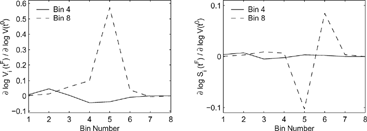
Figure 1 shows the logarithmic sensitivity coefficients of the mean volume densities in bins 4 and 8 at the end of the 48-h simulation interval with respect to the initial mean volume densities (left) and slopes (right). For both cases relative changes in the bin slopes have a considerably smaller influence on the final result than relative changes in the mean densities. The initial density of particles in bin 5 have the largest impact on the final density of large particles (bin 8). This means that after 48 h of evolution most of the large particles were formed through the growth and coagulation of particles that initially were in size bin 5. Conversely, the growth of particles from bin 5 to larger sizes has relatively small impact on the number density of particles in bin 4, hence, the sensitivities in bin 4 are small in comparison.

FIG. 1 The logarithmic sensitivities of the mean volume densities in bins 4 and 8 at final time with respect to the initial distribution bin averages (left) and bin slopes (right) for coagulation and growth.

The logarithmic sensitivities with respect to the values of the growth parameter σ and the coagulation parameter β are given in Table 1. The influences of relative perturbations in these parameters are of the same magnitude for both bins. Note that all sensitivity coefficients for each bin were obtained via a single adjoint integration.

TABLE 1 The logarithmic sensitivities of the mean volume densities in bins 4 and 8 with respect to the values of σ and β for coagulation and growth

	∂ log V/∂ log σ	∂ log V/∂ log β
Bin 4	−0.288	−0.178
Bin 8	−0.303	−0.406

Data Assimilation with Complete Observations

We first consider a complete set of hourly observations, that is, all parameters of the solution (mean concentrations and slopes in each bin) are observed once every simulation hour. The test problem consists of the evolution under both coagulation and growth. Coagulation-only and growth-only test results are similar and are discussed briefly at the end of this section.

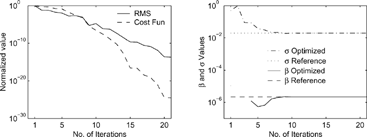
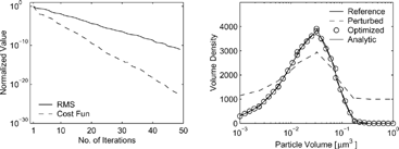
In Figure 2 the results for recovering the initial distribution are shown (the parameters β, σ assume reference values). The left plot shows the relative decrease of the cost function and RMS error with the number of iterations; the values of RMS and cost function are scaled by their initial value. We let the optimization routine run to convergence, and for the solution the RMS is decreased more than 10¹⁰ times from its starting value, and the cost function more than 10²⁰ times. The right plot shows the exact, reference, perturbed, and optimized distributions at the initial time. The optimized distribution is visually identical to the reference one. We also show the analytical distribution (round peak) which is well approximated by the numerical solution.

FIG. 2 Results for recovering the initial distribution for coagulation and growth from a complete set of observations.

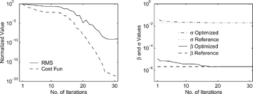
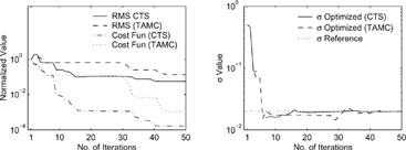
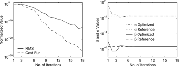
In Figure 3 the results for recovering β and σ are shown (the reference initial distribution is used in this experiment). The left plot shows the decrease of the cost function and RMS error with the number of iterations. The right plot shows the reference and optimized β, σ. As expected, the recovery of these 2 parameters require fewer iterations than the recovery of initial conditions (16 parameters).

FIG. 3 Results for recovering β and σ for coagulation and growth from a complete set of observations.

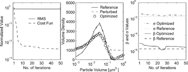
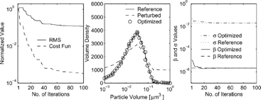
In Figure 4 the results for recovering simultaneously the initial distribution, β, and σ are shown. This experiment is more challenging for the inversion procedure since perturbations now affect not only the initial distribution, but the dynamic equation itself (through β and σ). The change of these parameters affects the evolution of the model throughout the simulation time interval. The left Figure 4 plot shows the decrease of the cost function and RMS error with the number of iterations. Note the modest decrease of RMS and cost function, and the large number of iterations. The central plot shows the exact, reference, perturbed, and optimized distributions at the initial time. The optimized distribution is visually identical to the reference one. The right plot shows the reference and optimized β and σ, which are recovered accurately.

FIG. 4 Results for recovering the initial distribution, β, and σ for coagulation and growth from a complete set of observations.

We have also performed separate experiments for growth only (recovering n ⁰, σ, and both) and coagulation only (recovering n ⁰, σ, and both) problems. The results are qualitatively similar to the ones presented in this section, and are not shown. The recovery of the parameters σ and β respectively is achieved in fewer than 10 iterations (RMS decreased more than 10¹⁰ times). The recovery of initial conditions is carried out in 15 iterations for coagulation, and 50 iterations for growth (RMS decreased more than 10¹⁰ times). For recovering both the initial distribution and the parameter (σ and β respectively) the optimization converges slower as expected.

Observations in Only Part of the Bins

In this section we present the performance of the data assimilation procedure when hourly measurements of number density are restricted to only a selected number of bins. We again consider the complete test problem with both coagulation and growth.

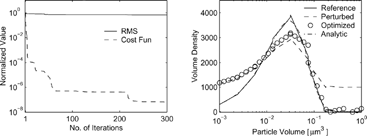
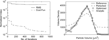
In Figure 5 the results for recovering the initial distribution without observations at bins 1, 2, and 3 are shown. The left plot shows the decrease of the cost function and RMS error with the number of iterations. Note the very large number of iterations needed, and the fact that, while the cost function decreases considerably, the RMS remains bounded below to about 10⁻¹. The right plot gives insight into this behavior. The initial distribution is recovered well overall, but the optimized values in bins 1 and 2 are inaccurate. For example, at bin 1 the bin average is correct but the slope is not. This is somewhat expected as the information in bins 1, 2, and 3 is not explicitly available to the optimization process. Additional experiments (not shown here) were carried out. The initial profile is recovered correctly with missing observations in bins 4 and 5 but shows consistent inaccuracies when observations in a large number of bins are missing. The conclusion is that it is possible to recover to a good extent the distribution of finer particles from the evolution equations, provided that enough observations of coarse particle are available.

FIG. 5 Results for recovering the initial distribution without observations at bins 1, 2, and 3 for both coagulation and growth.

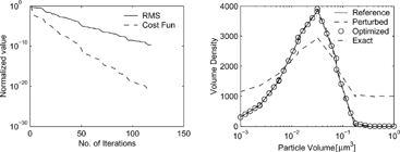
Figure 6 presents the results for recovering the initial distribution with observations at only even bins. The information provided by even bins is sufficient for an accurate recovery of the initial conditions. The complementary experiment (not shown here) of providing observations in only the odd-numbered bins leads to a good recovered initial profile, with some inaccuracies in the last bin (number 8).

FIG. 6 Results for recovering the initial distribution with observations at only even bins for both coagulation and growth.

The recovery of both parameters β and σ with observations at only bin 1 was tested, and the results are shown in Figure 7. The right panel shows the reference and optimized β and σ; note that, although the initial perturbations are very large, the reference values are recovered accurately with only several iterations. Additional experiments showed that the optimization process does not converge when observations are provided only in the large size bins (5–8), therefore the information in the lower size bins seems more important for the recovery of evolution parameters.

FIG. 7 Results for recovering β and σ with observations at bin 1 for both coagulation and growth.

The Impact of Observation Frequency

To assess the importance of observation frequency we repeat the experiments with observations in all bins available every 0.1 h, 1 h, 6 h, and 12 h. Figure 8 shows the RMS (left) and cost function (right) decrease with the number of iterations for these cases. Increasing the observation frequency below 1 hour does not seem to benefit the assimilation. Less frequent observations each 6 and 12 hours respectively impact the assimilation performance, but in both cases the optimization process converges. Note that for complex problems which include fast processes (chemistry and thermodynamics) a high observation frequency (below 1 hour) is expected to have a positive impact.

FIG. 8 Results for recovering the initial distribution from a complete set of observations with different frequencies. RMS error on the left, and cost function value on the right.

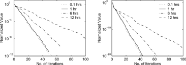
The results in Figure 8 should be compared with the results in Figures 5 and 6. The assimilation with relatively frequent, but incomplete observation is more difficult than the assimilation with infrequent but complete observations for the model problem under consideration.

Observations of Total Surface Density

Several tests were performed to recover the model parameters from hourly observations of total particle number, volume, and surface area per air volume, and for coagulation, growth, and coupled models. The results are qualitatively similar, therefore it is sufficient to only present the total surface density observations case for coupled coagulation and growth.

Figure 9 shows the results for recovering β and σ (with the evolution of the optimized values on the right). The parameters are recovered accurately after a relatively small number of iterations.

FIG. 9 Recovering β and σ from observations of total surface density.

The recovery of initial distributions is shown in Figure 10. While the cost function decreases as expected, the RMS stays flat for very large iteration numbers. The initial distribution in the large size bins is recovered fairly accurately, while the distribution in the lower size bins is hardly changed from the initial guess (perturbed value). This shows that in the logarithmic representation the small size bins span a much smaller physical volume range, and therefore contribute very little to the total surface density. Consequently total surface (number, volume) density observations contain more information on the large size bin densities (which are recovered) and little information on the small bin densities.

FIG. 10 Recovering the initial distribution from observations of total surface density.

Finally Figure 11 shows the results for simultaneously recovering the initial distribution, β, and σ. The optimized solution shows assimilation of the initial density in largest bin sizes, and an improvement in the β and σ values. The total surface density does not contain sufficient information for a complete recovery, and these parameters are still relatively far from the reference values, as are the initial densities in the lower bins.

FIG. 11 Recovering the initial distribution, β, and σ from observations of total surface density.

The results obtained with the current initial density are typical, that is, data assimilation of other initial density profiles will have the same qualitative behaviour.

Discrete versus Continuous Adjoints

To compare the influence of the choice of discrete versus continuous adjoint gradient on the performance of the optimization process we consider the growth-only test problem and repeat the data assimilation experiment (for both the initial density and σ) using a continuous adjoint gradient of the cost function. The continuous adjoint of the growth equation is also a growth (advection) equation, and the same Discrete Galerkin numerical solver was applied (note that in the volume density formulation used here the advection speed, or the growth rate, is constant). The results are shown in Figure 12. The continuous adjoint gradients lead to a faster convergence of the optimization process, as can be seen from the faster decrease in both cost function and RMS with the number of iterations (left plot). The value of the growth rate σ is also recovered in fewer iterations (right plot). This result is somewhat surprising as one would expect the derivative of the numerical solution, that is, the discrete adjoint, to be more accurate for optimization purposes.

FIG. 12 Recovering the initial distribution and σ for growth using continuous and discrete adjoint gradients. The continuous formulation leads to a better performance of the optimization process.

Direct versus Automatic Implementation of Discrete Adjoints

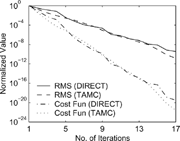
To assess the quality of the adjoints generated via automatic differentiation (TAMC) we compare their performance with a direct implementation of discrete adjoints as given by Equation (13). We consider the coagulation-only test case. The results presented in Figure 13 show that the optimization process performs similarly with both implementations, and requires a similar cpu time. This is expected since both approaches implement the same adjoint formulas, and the TAMC code is as efficient as the hand code for explicit time stepping.

FIG. 13 Recovering the initial distribution for coagulation using two implementations of the discrete adjoint gradients. The automatic differentiation and the direct implementation lead to similar performance.

CONCLUSIONS AND FUTURE WORK

In this paper we have developed the algorithmic tools needed for inverse aerosol modeling. Continuous and discrete adjoints of the integro-differential particle dynamic equation in number and mass concentration density formulations are derived. Formulas are obtained for the sensitivity coefficients of the solution with respect to the coagulation kernel, the growth rate, and emission and deposition coefficients.

The derivations are restricted to dynamics (without chemical and thermodynamic processes) and to zero dimensions (no transport processes). This is a first step toward performing data assimilation for comprehensive three-dimensional particle chemistry and transport models.

Comprehensive tests have been carried out using a single component particle dynamics model in a twin experiment framework. Pseudo-measurements are generated from a reference model run. From hourly measurements of the particle size one can recover the initial distribution as well as the parameters of the model. Measurements in only some of the bins provide enough information to recover the initial distribution and parameters. Measurements of total surface, volume, or number density are useful to adjust the unknown model parameters and initial conditions, and provide information mainly for the large size bins. Caution must be exercised when extrapolating these conclusions to the case of real observations, which are influenced by chemical and thermodynamic processes in addition to particle dynamics, and are corrupted by measurement errors. Aerosol data assimilation using real observations will be the focus of future work.

The overall conclusion is that 4D-Var data assimilation is a feasible approach for particle dynamics models. Discrete adjoints can be obtained easily through automatic differentiation, but continuous adjoints are also a viable alternative.

Testing of the computational tools developed in this paper is planned for more realistic models and a variety of evolution conditions. Data assimilation for a growth problem with three-component aerosols is presented in the companion paper (Henze et al. 2004). Future work will extend the inverse modeling of aerosols to include chemical and thermodynamic processes. The techniques developed will be used ultimately to perform data assimilation in full three-dimensional models.

APPENDIX A. DERIVATION OF THE CONTINUOUS ADJOINT OF THE DYNAMIC EQUATION IN NUMBER DENSITY FORMULATION

In this section we consider the general dynamic equation in number density formulation, with particle mass the independent variable:

where S(m,t) is any source of particles of mass m and L(m,t)n(m,t) is the first-order rate of removal of particles of mass m. The cost functional to be minimized is expressed in the general, integral form

We will use the Lagrangian multiplier method to derive the continuous adjoint equations and sensitivities with respect to all parameters. We define the cost functional as

Here LHS _n and RHS _n refers to the left side and right side of Equation (A.1), respectively. J ₀ is the local cost functional component. We take variation of the functional (A.3) and obtain

By exapnding the above equation, integrating by parts, and rearrranging, the variation δ can be written as:

where

and

If the Lagrange multiplier λ is chosen as the solution of the adjoint equation

then the term = 0.

To deal with the terms −∫₀ ^∞ λ(m,t) δ n(m,t)| _{t 0} ^T dm, ∫ _{t 0} ^T δ I(m,t)n(m,t)λ(m,t)|₀ ^∞ dt and ∫ _{t 0} ^T δ n(m,t)I(m,t)λ(m,t)|₀ ^∞ dt, we impose the following boundary and initial conditions

Then the variation δ simplifies to

Therefore the values of the functional sensitivities are:

APPENDIX B. DERIVATION OF THE CONTINUOUS ADJOINT OF THE DYNAMIC EQUATION IN MASS DENSITY FORMULATION

We consider the dynamic equation in mass density for components i = 1,2,…,r:

where the source term m _i S(m,t) and the removal term L(m,t)q _i (m,t) have the same units. m = ∑ _{i = 1} ^r m _i , q(m,t) = ∑ _{i = 1} ^r q _i (m,t), H(m,t) = ∑ _{i = 1} ^r H _i (m,t).

We use the Lagrange multiplier method to derive the continuous adjoint equation considering perturbations in all parameters. The cost functional is defined as

Here LHS _qi and RHS _qi refers to the left side and right side of Equation(B.1), respectively. J ₀ is the local cost functional component.

Taking the variation of Equation (B.2) gives

After integrating by parts and rearranging δ can be written in a compact form:

where

and

Imposing A _i = 0 leads to the adjoint equation

Then

Therefore,

APPENDIX C. DERIVATION OF THE DISCRETE ADJOINT OF THE DYNAMIC EQUATION

For an ordinary differential equation

and a cost functional

the continuous adjoint equation reads

Here f _y denotes the Jacobian of f with respect to y. Note that the adjoint equation depend on the state variable y of the forward equation.

For the Forward Euler discretization and a discrete in time cost function

the discrete adjoint equation is obtained from the interpretation of adjoint variables as derivatives of the cost functional and the application the transposed chain rule

In the above derivation we used the causality, that is, the fact that y ^k does not depend on y ^j for j < k. In practice the times where the cost functional is defined are multiples of the discretization time step, and the factor δ^obs _k equals 1 if t ^k is a time used in the definition of the cost functional, and equals 0 otherwise.

The numerical experiments presented in this paper use the two stage, second order, strongly stable, explicit Runge Kutta method

The discrete adjoint can be derived using an approach similar to the one used for Forward Euler

The discrete adjoints for the particle dynamic equation are obtained by applying this formulation with the Jacobian f _n ^T of the semidiscrete Equation (3)

where

APPENDIX D. DERIVATION OF THE DISCRETE ADJOINT OF THE SEMI-IMPLICIT METHOD

In this section we derive the discrete adjoint of the popular semi-implicit method for solving the coagulation equation. In this approach the particles are divided in s bins, and all particles in bin i have the same volume v _i . The coagulation of particles of volumes v _i and v _j forms particles of volume V _i,j = v _i + v _j . These particles are distributed to the nearest bins, a fraction f _i,j,k going to bin k, and the reminder going to bin k−1. The fraction coefficients are defined as:

The number concentration in bin k at time t ^ℓ is denoted by n _k ^ℓ. The concentration changes during one time step t ^ℓ+1 = t ^ℓ + δ t by the formula

This equation is solved iteratively for k = 1… s.

To derive the discrete adjoint consider again the transposed chain rule

From (D.1),we can derive that

Introduce the notations

The Equation (D.3) can be written as

From (D.2) and (D.4)

or equivalently

Since D ^T is an upper triangular matrix the system in z can be solved by a backwards substitution, in the same fashion the forward equation is solved. The complete adjoint formula is therefore

Acknowledgments

The authors thank the National Science Foundation for supporting this work through the award NSF ITR AP&IM 0205198. The work of A. Sandu was also partially supported by the award NSF CAREER ACI 0093139.

REFERENCES

- Mathematics and Computer Science Division at Argonne National Laboratory and the Center for Research on Parallel Computation at Rice University . Automatic Differentiation of Fortran , http://www-unix.mcs.anl.gov/autodiff/ADIFOR/
- Binkowski , F. S. and Shankar , U. 1995 . The Regional Particulate Matter Model: 1: Model Description and Preliminary Results . Journal of Geophysical Research. , 100 : 26,191 – 26,209 .
- Bott , A. 1989 . A Positive Definite Advection Scheme Obtained by Nonlinear Renormalization of the Advection Fluxes . Monthly Weather Review. , 117 : 1006 – 1115 . [CSA] [CROSSREF]
- Byrd , A. , Lu , P. and Nocedal , J. 1995 . A Limited Memory Algorithm for Bound Constraint Optimization . SIAM Journal on Scientific Computing , 16 : 1190 – 1208 . [CROSSREF]
- Carmichael , G. R. , Daescu , D. , Sandu , A. and Chai , T. June 2003 . “ Computational Aspects of Chemical Data Assimilation into Atmospheric Models, ICCS03 ” . In Springer Lecture Notes in Computer Science , Vol. 2660 , June , pp. 269 – 278 . Melbourne, , Australia : Springer-Verlag GmbH .
- Corliss , G. , Faure , C. , Griewank , A. , Hascoet , L. and Naumann , U. 2001 . Automatic Differentiation of Algorithms, from Simulation to Optimization Springer LNCSE series
- Courty , F. , Araya , M. , Vazquez , M. , Pascual , V. , Dervieux , A. , Bellesso , N. , Hascoet , L. and Greborio , R. 2003 . Tapenade On-line Automatic Differentiation Engine , France : INRIA . http://www-sop.inria.fr/tropics/index.html
- Daescu , D. , Sandu , A. and Carmichael , G. R. 2003 . Direct and Adjoint Sensitivity Analysis of Chemical Kinetic Systems with KPP: II—Validation and Numerical Experiments . Atmospheric Environment , 37 : 5097 – 5114 . [CROSSREF]
- Elbern , H. , Schmidt , H. and Ebel , A. 1997 . Variational Data Assimilation for Tropospheric Chemistry Modeling . J. Geophysical Research , 102 ( D13 ) : 15967 – 15985 . [CSA] [CROSSREF]
- Gelbard , F. M. and Seinfeld , J. H. 1978 . Coagulation and Growth of a Multicomponent Aerosol . J. Colloid and Interface Science , 63 ( 3 ) : 472 – 479 .
- Gelbard , F. M. and Seinfeld , J. H. 1996 . Coagulation and Growth of a Multicomponent Aerosol . J. Colloid and Interface Science , 63(3) : 472 – 479 .
- Giering , R. 1997 . Tangent Linear and Adjoint Model Compiler . Users Manual Manual ,
- Giering , R. and Kaminski , T. 1998 . Recipes for Adjoint Code Construction Article . ACM Trans. Math. Software ,
- Giering , R. Tangent linear and Adjoint Model Compiler . http://www.autodiff.com/tamc
- Griewank , A. , Juedes , D. and Utke , J. 1996 . ADOL–C, A Package for the Automatic Differentiation of Algorithms Written in C/C++ Article . ACM Trans. Math. Software , http://www.math.tu-dresden.de/wir/project/adolc/index.html
- Griewank , A. 2000 . Evaluating Derivatives: Principles and Techniques of Algorithmic Differentiation Frontiers in Applied Mathematics .
- Henze , D. K. , Seinfeld , J. H. , Liao , W. , Sandu , A. and Carmichael , G. R. 2004 . Inverse Modeling of Aerosol Dynamics: Condensational Growth . J. Geophys. Res. , 109 : D14 [CROSSREF]
- Jacobson , M. Z. 1997 . Numerical Techniques to Solve Condensational and Dissolutional Growth Equations When Growth is Coupled to Reversible Reactions . Aerosol Sci. Technol. , 27 : 491 – 498 .
- Jacobson , M. Z. 1999 . Fundamentals of atmospheric modeling , New York : Cambridge University Press .
- Kim , Y. P. and Seinfeld , J. H. 1990 . Simulation of Multicomponent Aerosol Condensation by the Moving Sectional Method . J. Colloid and Interface Science. , 135 ( 1 ) : 185 – 199 . [CROSSREF]
- Lurmann , F. W. , Wexler , A. S. , Pandis , S. N. , Musara , S. , Kumar , N. and Seinfeld , J. H. 1997 . Modeling Urban and Regional Aerosols - ii. Application to California's South Coast Air Basin . Atmos. Environ. , 31 : 2695 – 2715 . [CROSSREF]
- Meng , Z. , Dabdub , D. and Seinfeld , J. H. 1998 . Size-Resolved and Chemically Resolved Model of Atmospheric Aerosol Dynamics . J. Geophysical Research. , 103 ( D3 ) : 3419 – 3435 . [CSA] [CROSSREF]
- Naumann , U. , Christianson , B. and Riehme , J. Automatic Differentiation Differentiation Enabled Fortran Compiler Technology . NAGWare Fortran 95, http://www.nag.co.uk/nagware/research/ad_overview.asp
- Nguyen , K. and Dabdub , D. 2001 . Two-Level Time-Marching Scheme Using Splines for Solving the Advection Equation . Atmos. Environ. , 35 : 1627 – 1637 . [CROSSREF]
- Nguyen , K. and Dabdub , D. 2002 . Semi-Lagrangian Flux Scheme for the Solution of the Aerosol Condensation/Evaporation Equation . Aerosol Sci. Technol. , 36 : 407 – 418 . [CROSSREF]
- Nocedal , J. 1980 . Updating Quasi-Newton Matrices with Limited Storage . Mathematics of Computation , 35 : 773 – 782 .
- Nocedal , J. Department of Electrical & Computer Engineering, Northwestern University . http://www.ece.northwestern.edu/nocedal/lbfgs.html
- Pilinis , C. 1990 . Derivation and Numerical Solution of the Species Mass Distribution Equation for Multicomponent Particulate Systems . Atmos Environ. , 24A ( 7 ) : 1923 – 1928 .
- Sandu , A. 2002 . A Newton-Cotes Quadrature Approach for Solving the Aerosol Coagulation Equation . Atmos. Environ. , 36 : 583 – 589 . [CROSSREF]
- Sandu , A. and Borden , C. T. 2003 . A Framework for the Numerical Treatment of Aerosol Dynamics . Applied Numer. Math. , 45 : 475 – 497 . [CROSSREF]
- Sandu , A. , Daescu , D. and Carmichael , G. R. 2003 . Direct and Adjoint Sensitivity Analysis of Chemical Kinetic Systems with KPP: I—Theory and Software Tools . Atmos. Environ. , 37 : 5083 – 5096 . [CROSSREF]
- Sandu , A. 2004 . Piecewise Polynomial Solutions of Aerosol Dynamics . Submitted
- Sandu , A. , Daescu , D. , Chai , T. , Carmichael , G. R. , Seinfeld , J. H. , Hess , P. G. and Anderson , T. L. 2004 . “ Computational Aspects of 4D-Var Chemical data Assimilation in Atmospheric Models ” . In Dynamic Data Driven Applications Systems , Edited by: Darema , F. Kluwer Academic Publishers .
- Sandu , A. , Daescu , D. , Carmichael , G. R. and Chai , T. 2005 . Adjoint Sensitivity Analysis of Regional Air Quality Models . J. Computational Physics , 204 : 222 – 252 . [CROSSREF]
- Seinfeld , J. H. and Pandis , P. N. 1997 . Atmospheric Chemistry and Physics. From Air Pollution to Climate Change , New York : John Wiley & Sons .
- Tsang , H. and Hippe , J. M. 1988 . Asymptotic Behavior of Aerosol Growth in the Free Molecule Regime . Aerosol Sci. Technol. , 8 : 265 – 278 . [CSA]
- Zhang , Y. , Seinfeld , J. H. , Jacobson , M. Z. and Binkowski , F. S. 1999 . Simulation of Aerosol Dynamics: A Comparative Review of Algorithms Used in Air Quality Models . Aerosol Sci. Technol. , 31 : 487 – 514 . [CROSSREF]