Major Source Categories for PM_2.5 in Pittsburgh using PMF and UNMIX

An objective of the Pittsburgh Air Quality Study was to determine the major sources of PM_2.5 in the Pittsburgh region. Daily 24-hour averaged filter-based data were collected for 13 months, starting in July 2001, including sulfate and nitrate data from IC analysis, trace element data from ICP-MS analysis, and organic and elemental carbon from the thermal optical transmittance (TOT) method and the NIOSH thermal evolution protocol. These data were used in two source-receptor models, Unmix and PMF. Unmix, which is limited to a maximum number of seven factors, resolved six source factors, including crustal material, a regional transport factor, secondary nitrate, an iron, zinc and manganese factor, specialty steel production and processing, and cadmium. PMF, which has no limit to the number of factors, apportioned the PM_2.5 mass into ten factors, including crustal material, secondary sulfate, primary OC and EC, secondary nitrate, an iron, zinc and manganese factor, specialty steel production and processing, cadmium, selenium, lead, and a gallium-rich factor. The Unmix and PMF common factors agree reasonably well, both in composition and contributions to PM_2.5. To further identify and apportion the sources of PM_2.5, specific OC compounds that are known markers of some sources were added to the PMF analysis. The results were similar to the original solution, except that the primary OC and EC factor split into two factors. One factor was associated with vehicles as identified by the hopanes, PAH's, and other OC compounds. The other factor had strong correlations with the OC and EC ambient data as well as wood smoke markers such as levoglucosan, syringols, and resin acids.

INTRODUCTION

Elevated levels of PM_2.5 have been linked to human health effects (e.g., Dockery et al. 1993; Pope et al. 2002). Upon establishment of a National Ambient Air Quality Standard for PM_2.5 in 1997 (US EPA 1997a), many urban areas find themselves to be in non-attainment of the PM_2.5 standard. Effective air pollution control strategies for PM_2.5 require investigation into its sources, composition, and spatial and temporal variations. The Pittsburgh Air Quality Study (PAQS) was a multidisciplinary set of projects in the Pittsburgh region designed to address these issues. PAQS program objectives, hypotheses, site description, and measurement methods are described in Wittig et al. (2004). In this paper, data collected during the PAQS are analyzed with two commonly used source-receptor models, Unmix and Positive Matrix Factorization (PMF), to determine the major source categories and their contributions to ambient concentrations of PM_2.5.

The main contributions of this paper are (1) a source apportionment for Pittsburgh PM_2.5, (2) a comparison of the PMF and Unmix models, and (3) evaluation of PMF results upon addition of individual organic markers. Several studies of the sources of PM_2.5 in Pittsburgh have been conducted as a part of the PAQS; however, they have been focused on measurements from one instrument or analysis technique or a small set of the components of PM_2.5. Source apportionment of the carbon fraction of PM_2.5 has been reported for Pittsburgh (Subramanian 2004). Source-receptor modeling based on one month or less of sampling has been conducted (Modey et al. 2005; Zhou et al. 2004). And composition of single particles in an effort to identify sources of the particles has been explored (Lithgow et al. 2004). This paper describes source-receptor modeling with a larger dataset such that more factors and their seasonal variations can be identified. PMF and Unmix comparisons have been conducted in other studies (Maykut et al. 2003; Kim et al. 2004; Poirot et al. 2001; Larsen and Baker 2003; Eatough et al. 2005) with varying results. Confidence in using these two receptor modeling tools is gained with convergent results, whereas divergent results signify limitations in the data or models. Trace elements have been used in many receptor modeling studies due to the assumption that they can serve as tracers for some sources. However, most elements can be emitted from multiple types of sources, and thus identifying factors based on their correlation with elemental data is difficult. Molecular markers have been shown to be good tracers of certain sources (Schauer and Cass 2000; Schauer et al. 1996; Simoneit et al. 1999; Subramanian et al. 2005b). This paper discusses the use of both elemental species and molecular markers in a PMF analysis in an effort to improve the interpretation of factors as well as to resolve more factors than a PMF analysis using elemental tracers alone.

EXPERIMENTAL AND METHODOLOGY SECTION

Site Description

All samples in this study were collected at the PAQS main monitoring station. The station was located approximately 6 km east of downtown Pittsburgh in a park, where impact from local sources was minimized. Sampling equipment was housed on the roof of a trailer, approximately 5 m from the ground. Samples were collected daily from July 2001 through September 2002 although only data collected from July 2001 to July 2002 have been used in this study. Site and project details are described more completely in Wittig et al. (2004).

Sampling and Analysis

Ambient concentration data used in the source-receptor modeling include total ambient PM_2.5 mass, sulfate, nitrate, total organic carbon (OC), elemental carbon (EC), and trace elements. These species represent the major constituents of PM_2.5 in Pittsburgh with the exception of ammonium (Rees et al. 2004). Total number of missing and below detection limit values are summarized in Table 1 for each species.

TABLE 1 Summary of the dataset for PMF and Unmix use. All considered species are listed; not all species were used in the two models. Number of values below the minimum detection limit (MDL) and number of missing values are given out of a total of 386 sampling dates

PM2.5 species	Number of values below MDL	Number of missing values
Total PM2.5	0	45
Sulfate	0	20
Nitrate	0	9
OC	0	1
EC	0	1
Ag	230	5
As	5	5
Ba	69	5
Be	278	5
Ca	191	5
Cd	45	5
Ce	260	57
Co	175	5
Cr	63	5
Cs	295	5
Cu	122	5
Fe	31	5
Ga	95	5
K	41	5
Li	189	5
Mg	115	5
Mn	5	5
Mo	42	5
Ni	72	5
Pb	5	5
Rb	124	5
Sb	14	5
Se	4	5
Sr	95	5
Ti	30	5
Tl	238	5
V	22	5
Zn	38	5

PM_2.5 Mass

Samples were collected on 47 mm Teflon filters (Whatman No: 7592-104) using a Partisol®-FRM Model 2000 PM_2.5 Air Sampler (Rupprecht & Pataschnick Co., Inc.). Semi-continuous PM_2.5 mass was measured using a Tapered Element Oscillating Microbalance (TEOM) monitor with a Sample Equilibration System (SES) (Rupprecht and Patashnick, Model 1400A). Data from the TEOM were averaged to get 24-hour measurements. The 24-hour averaged data from the two PM_2.5 mass measurement methods agree well with a linear regression R² value of 0.95, a slope of 1.02 and an intercept of 0.65 (Rees et al. 2004). However, the TEOM recorded fewer missing dates, hence the data collected by the TEOM will be used in this study.

Sulfate and Nitrate

A PM_2.5 sampler with cyclones, denuders and filter packs containing PTFE Teflon, nylon, and cellulose filters was used to collect daily 24-hour averaged samples. The material collected on the filters was extracted in deionized water and the solution was analyzed for nitrate, nitrite, sulfate, chloride, ammonium, and sodium by Ion Chromatography (IC) (Takahama et al. 2004).

OC and EC

PM_2.5 samples were collected on quartz filters using a cyclone/filter pack sampler (Subramanian et al. 2004). The quartz filters were analyzed for OC and EC using the Thermal Optical Transmittance (TOT) method and the NIOSH thermal evolution protocol (NIOSH 1996; Cabada et al. 2004). Because the OC data are used in a mass balance application, an OC multiplier is applied to the measurements to approximate total organic mass. Most mass balance studies use a value of 1.4 for the OC multiplier. Based on recent work by Polidori et al. (2005) and Turpin and Lim (2001) and the hypothesis that the air quality in Pittsburgh is dominated by regional transport (Tang et al. 2004; Anderson et al. 2004), a multiplication factor of 1.8, which is representative of an aged, regional aerosol, was used to estimate total organic mass from OC measurements.

Trace Elements

A Thermo Andersen PM_2.5 high volume sampler (hi vol) was used to collect daily 24-hour averaged filter-based samples from July 11, 2001 through July 31, 2002. Samples collected on Whatman 41 cellulose filters were cut into sections, and digested in a laboratory microwave in closed vessels containing a solution of nitric/hydrofluoric acid and hydrogen peroxide. The sample preparation and subsequent analysis by ICP-MS were verified to be accurate by testing recovery of a NIST standard reference material (Pekney and Davidson 2005). Measured elements include Ag, As, Ba, Be, Ca, Cd, Ce, Co, Cr, Cs, Cu, Fe, Ga, K, Li, Mg, Mn, Mo, Ni, Pb, Rb, Sb, Se, Sr, Ti, Tl, V, and Zn. Minimum detection limits (MDLs), calculated for each sample, were defined as 3.3σ _B/V, where σ _B is the uncertainty in the field blank measurements and V is the volume of air sampled (US EPA 1997b).

The Unmix Model

Unmix is a commonly used source-receptor model (Henry 1997, 2001) based on the assumption that each source of unknown composition contributes an unknown amount to each sample collected. The model uses a principal component analysis to solve the general equation

where x is the matrix of ambient data collected at the receptor site, consisting of the species in columns and dates in rows. The matrix f is the gravimetric mass of each element j per unit PM mass emitted from each source k, or source compositions, and g is the matrix of the fraction of total PM_2.5 ambient concentration from source k in sample i, or source contributions. The goal is to find f and g by minimizing the residual error, e, which accounts for error in the model fit. Uncertainty in the data is not considered by the model, which implicitly assumes a certain standard of accuracy in the data for a good model fit. There are an infinite number of solutions to Equation (1), so the model restricts solutions to those that are physically meaningful in that factor compositions and contributions are non-negative. Also, the sum of the concentrations of an element from all factors in one day cannot be greater than the measured mass concentration of the element for that day. The model operates under the assumption that the data form well-defined “edges,” meaning that each factor, when plotted against another, will have some dates during which the contribution is zero for one factor and non-zero for the other factor, creating an edge in a multi-dimensional space. The results are limited to a maximum of seven factors but the user must select which measured species to use in the model. The model does not use data from any date from which one or more species concentrations are missing.

PMF Model

The 2-dimensional PMF model, PMF2, solves Equation (1) by a weighted least-squares fit with the known error estimates of the elements of matrix x used to derive the weights (Paatero and Tapper 1993, 1994; Paatero 1997). PMF minimizes Q, defined as

where s_ij are the error estimates for the elements in x described above. Ideally Q would have e_ij approximately equal to s_ij, producing a value of n × m, the number of values in the data matrix x or the number of degrees of freedom. The same non-negativity constraints from Unmix apply to PMF. Because PMF has provision to incorporate uncertainty in the data into the model, data sets with missing values can be used by applying a large uncertainty so that the missing data will have negligible influence on the model results. Missing data can be approximated as the geometric mean of the corresponding element concentration with an uncertainty of 4 times the geometric mean (Polissar et al. 1998).

Uncertainty estimates for the s matrix were determined as follows for each of the species included in the model. For trace element data above the minimum detection limit (MDL), uncertainty in the ambient concentrations was determined by compounding errors from the most uncertain components: the volume of air sampled, contamination as reflected in the field blanks, and the variation in element mass measured on two or three different sections from each filter. For data below the MDL, the concentration was approximated as one half the sample MDL, with an assigned uncertainty of one half the sample MDL plus one-third the study-average MDL for the corresponding element according to Polissar et al. (1998). Uncertainty in the sulfate and nitrate data was calculated from propagation of error in the volume of air sampled, the variation in the field blanks, the extraction volume, and the variation in replicate analyses. Uncertainty in the OC and EC data was calculated from propagation of error in the volume of air sampled and the variation in the replicate analyses of collected samples. In this study, a third of the MDL was added to the analytical uncertainty for each value above the MDL (Polissar et al. 1998).

The non-negativity constraint decreases the rotational freedom, but with many datasets, more than one solution still exists. The parameter FPEAK allows manipulation of the g and f matrices (Equation (1)) such that rotational freedom in the model can be examined. Selection of the number of factors, or sources, requires some subjectivity. The user must select a maximum number of factors that can adequately describe the total PM_2.5 mass while excluding factors that do not make physical sense, such as duplicate factors or factors with unrealistic compositions or contributions. This requires some knowledge of the quality of the data and the source types in the area. Evaluating multiple solutions within the range of FPEAK values that yield an acceptable Q value and assessing the edge plots are more objective ways to evaluate the model results.

RESULTS AND DISCUSSION

Unmix Model Results

The Unmix model created a six-factor solution with the source compositions shown in Figure 1 and source contributions shown in Figure 2. Some combinations of the species considered resulted in a solution that was not feasible. The combination of species that provided the best solution included Ca, Ti, Cr, Mn, Fe, Zn, Mo, Cd, sulfate, nitrate, OC, and EC. Three parameters designed to evaluate the model results are the minimum R², the signal-to-noise ratio, and the strength. The R² value is related to the proportion of variance of each species explained by the factors. For all species, the minimum R² value is recommended to be greater than 0.8. For the selected species, the minimum R² value was 0.86. The minimum signal-to-noise ratio is the smallest estimated signal-to-noise ratio for any of the factors in the model, recommended to be greater than 2. A value of 2.32 was obtained using this dataset. The strength is a measure of the confidence in the model. Strength is recommended to be greater than 3, but with some datasets this is unachievable and thus a strength less than 3 may still be acceptable (Henry, personal communication). For this dataset, it was impossible to find a combination of species yielding a strength greater than 3, and the final solution had a strength of 1.41.

FIG. 1 Unmix source compositions apportioned by PM_2.5 mass. All ten factors are outputs of PMF, while only the first six factors are outputs of Unmix. Although the Unmix regional transport factor includes primary OC and EC, it is graphed for comparison with the PMF sulfate factor.

FIG. 2 PMF and Unmix source contributions apportioned by PM_2.5 mass. All ten factors are outputs of PMF, while only the first six factors are outputs of Unmix. Note that for comparison purposes, the Unmix regional transport factor is compared to the PMF sulfate plus primary OC and EC factors.

Species for which the ambient data correlated strongly with the source contributions (correlation coefficient greater than 0.7) allow determination of the source types. The six factors in the model have been designated a crustal material factor, a regional transport factor, a nitrate factor, an Fe, Mn, and Zn factor, a specialty steel production factor, and a cadmium factor. Descriptions of the nature of the factors, such as their contributions to PM_2.5 mass on a seasonal basis as well as a yearly average, are given below. To determine the mass contribution to PM_2.5, the total PM_2.5 mass was included as a species in the model, and the calculated source compositions and contributions were normalized by the Unmix-apportioned PM_2.5 mass. Because PM_2.5 is used as a fitting species, together these six factors account for all of the PM_2.5 mass. Figure 3 shows the Unmix source contributions normalized by the Unmix-apportioned PM_2.5 mass, averaged monthly and for the entire study.

FIG. 3 Monthly average Unmix source contributions. Height of the bars corresponds to the monthly average PM_2.5 mass measured with a TEOM. The study average represents the average source contributions from July 11, 2001 through July 31, 2002. Unmix uses PM_2.5 mass as a fitting species so the mass of PM_2.5 unexplained by Unmix is less than 1%.

Crustal Material Factor

The crustal material factor, with Ca and Ti tracers, contributes 13% to the PM_2.5 on an annual average. The factor is composed of 46% OC, 34% sulfate, 7% EC, 6% nitrate, 3% Fe, and 2% Ca. The high concentrations of sulfate and OC in the factor indicate the resuspended crustal material includes noncrustal deposited material, presumably of anthropogenic origin. Seventy-three percent of the Ca mass, 71% of the Ti mass, and 36% of the Fe mass is explained by this factor. Crustal material is present in PM_2.5 from weathering of rocks and soil. Typically most of the mass of crustal elements such as calcium and titanium is found in larger particles, but Unmix can still identify this factor using only PM_2.5 data. Seasonally, the crustal material source contribution is slightly higher during the first five months of the study in the summer/fall, but overall no consistent seasonal trend was observed.

Regional Transport Factor

This factor, with sulfate, OC, and EC tracer species, contributes 68% of the PM_2.5 mass on an annual average, making it by far the largest source category. The factor is mostly composed of 61% sulfate, 36% OC, and 2% EC, and accounts for 84% of the sulfate mass, 54% of the OC mass, and 37% of the EC mass. Sulfate is a major component of ambient PM_2.5 in the Pittsburgh region, comprising 38% on an annual average (Rees et al. 2004). Many coal-fired power plants are located in the Ohio River Valley south and southwest of the monitoring station. These sources emit large amounts of SO₂ as well as some coal fly ash. The SO₂ is oxidized to eventually form particulate sulfate, making this category predominantly secondary material. Because Pittsburgh is frequently downwind, these sources are suspected to contribute significantly to the regional nature of Pittsburgh's air pollution (Tang et al. 2004; Anderson et al. 2004). Based on the available data Unmix is unable to separate the secondary sulfate, usually associated with some secondary OC, from the primary OC and EC, associated with many different sources, including vehicular emissions. EC is emitted from diesel engines, but because of the same location of the vehicular sources (gas and diesel) and the same meteorology affecting the concentrations at the receptor site, Unmix is unable to separate the gasoline engine source profile from the diesel engine profile. Application of Unmix to multi-sample/day data from Pittsburgh for July 2001 did allow separation of the sulfate, diesel and gasoline sources (Modey et al. 2005). The information on the diurnal data probably aided in this separation of sources. EC may also be associated with biomass burning, which is not a major source of PM_2.5 in the Pittsburgh region (Cabada et al. 2002). Therefore this factor is dominated by regionally transported secondary sulfate and OC and includes primary OC and EC emissions as well. The contribution of this factor to total PM_2.5 is higher in the summer than in the winter due to the increase in photochemistry that favors formation of particulate sulfate.

Nitrate Factor

This factor is also attributed to a secondary source, as the tracer, nitrate, is a secondary pollutant. The factor is mostly composed of 41% nitrate and 40% OC, and accounts for 80% of the nitrate mass and 17% of the OC mass. The major source of nitrate is conversion of NO_x from high-temperature combustion, such as internal combustion engines in cars. The significant OC associated with this factor could reflect secondary organic material formed at the same time as the nitrate. The source contribution is highest in the winter months as expected, when lower temperatures favor nitrate particles rather than nitric acid vapor. The higher winter contribution could also reflect lower mixing heights and the increased importance of local sources. The nitrate factor is second largest, with an annual average contribution of 14% to PM_2.5.

Iron, Manganese, and Zinc Factor

This factor has tracer species of Fe, Mn, and Zn, while the bulk of the factor (70%) is composed of OC. Most of the Fe, Mn, and Zn masses are attributed to this factor (49%, 67%, and 78%, respectively). These elements are quite common in a number of source categories, including steel mills, vehicles, waste incinerators (Zn), soil dust, and even coal combustion (Parekh 1990; Olmez et al. 1988; Watson et al. 2001). Blast furnaces and steel mills produce emissions of iron, manganese, and zinc and there are several in the area (US EPA 2002). Iron ore is a raw material used for making steel, manganese is an alloying element, and zinc is used for coating and galvanizing steel (AISI 2004). This factor is likely to represent emissions from the steel production industry. The source contribution does not show a seasonal trend, and annual average contribution to PM_2.5 is 4% for this factor.

Specialty Steel Factor

Mo and Cr are the tracer species for this factor, most of which is composed of 65% OC and 19% EC. Both chromium and molybdenum are used as alloying elements in specialty steel; together these elements enhance the corrosion resistance of stainless steel (AISI 2004). The Pittsburgh region has many specialty steel processing and finishing facilities. The Unmix factor marked by molybdenum and chromium is assumed to be associated with these facilities; however, it is a minor factor, contributing less than 1% to the annual average PM_2.5. No seasonal trend in contribution is observed.

Cadmium Factor

This factor, with a Cd tracer, is minor in PM_2.5 contribution, approximately 1% on an annual average. Factor composition is 60% sulfate, 17% OC, and 13% nitrate, and 82% of the Cd mass is explained by this factor. The contribution of the cadmium factor is almost always quite low except for a few large peaks. This may indicate a local source, possibly a point source whose plumes only impact the site on a few days out of a year. Other source-receptor studies that include cadmium generally show this element in association with other species rather than by itself, suggesting that Pittsburgh has a different mix of cadmium sources than other locations.

PMF Model Results

The robust mode, rather than the default mode, was selected to handle outliers in the data. The robust factorization iteratively reweighs individual values such that the minimization of Q now becomes

where

A typical value of α = 4 was chosen. To apportion each factor by mass, typically a scaling constant S normalizes the source contributions. The value of S is determined by a multiple linear regression of the sum of concentrations of the component species in a sample versus the sum of modeled source contributions for that sample, or the observed versus the predicted PM_2.5. However, as shown in Figure 4, the sum of species concentrations plotted against the total PM_2.5 mass concentration as measured by the TEOM shows agreement that worsens at higher concentrations. The sums of species concentrations, including PM_2.5 sulfate, nitrate, OC (multiplied by 1.8), EC, and the trace elements used in the PMF analysis (see Figure 5), are on average lower than the total PM_2.5 mass concentration. Reasons for this discrepancy have been explored in detail in Rees et al. (2004). Because of the lack of mass balance closure, total PM_2.5 measured mass concentration was included as a species in the model so that PMF could apportion the mass directly. PM_2.5 uncertainty was set at 4 times the concentration to decrease its weight in the model fit (Kim et al. 2003). The source contributions and compositions were then normalized by the PM_2.5mass concentration apportioned to each factor to get quantitative results.

FIG. 4 Mass balance. Sum of the species concentrations used in the PMF analysis vs. the total PM_2.5 mass as measured by the TEOM. A linear regression of the data shows an R² value of 0.76. The regression slope of 1.49 shows that the line is biased high as expected, since PMF could not identify the sources of all of the PM_2.5 mass.

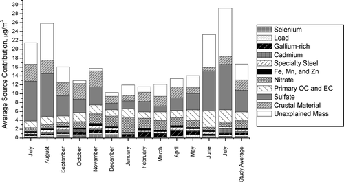
FIG. 5 Monthly average PMF source contributions. Height of the bars corresponds to the monthly average PM_2.5 mass measured with a TEOM. The study average represents the average source contributions from July 11, 2001 through July 31, 2002. The unexplained mass is the difference between the monthly average PM_2.5 mass and the sum of the monthly averaged source contributions from each factor.

A detailed examination of model results and goodness-of-fit were carried out for models with 8–12 solutions. An analysis of the effects of changing the FPEAK value from –0.8 to + 0.8 showed that the change in rotation did not have a very significant effect on the results. A 10-factor model provided the most realistic results. The actual Q value was 8884 as compared to the theoretical value of 8878.

G-space plotting, similar to the edge plots from the Unmix model, involves forming scatter plots of pairs of source contribution factors (Paatero et al. 2005). The solution can be rotated to achieve the optimal solution, which has edges that lie on or parallel to the two axes for all scatter plots. A value of –0.2 was chosen for FPEAK: although the Q-value did not change significantly from the no-rotation solution, several of the edges in the edge plots improved with this slight rotation.

PMF allows inclusion of more species in the model due to the consideration of uncertainties that enables handling of missing and below detection limit data. Species included in the PMF solution are PM_2.5 sulfate, nitrate, OC, EC, Mg, K, Ca, Ti, V, Cr, Mn, Fe, Ni, Cu, Zn, Ga, As, Se, Mo, Cd, Ba, and Pb. We can identify a tracer species for each factor based on the source compositions shown in Figure 1. However, a better indication is the correlation of the species ambient concentration with the PMF-modeled source contribution. A correlation greater than 0.7 is a good indication of a tracer species. Based on the tracer species for each factor, the factors were defined as crustal material (Ca and Ti tracers), sulfate, nitrate, an Fe, Zn, and Mn factor, specialty steel (Mo and Cr tracers), cadmium, a gallium-rich factor, lead, selenium, and primary OC and EC (OC and EC tracers).

Description of PMF Sources

A comparison of compositions and contributions for factors found by both Unmix and PMF are shown in Figure 1 and Figure 2. These source categories include crustal material, sulfate, nitrate, steel production, specialty steel, and cadmium. The factors not found by Unmix but found by PMF are described below, and their source compositions and contributions are also shown in Figure 1 and Figure 2. Figure 5 shows the average PMF source contributions apportioned by average PM_2.5 mass concentration. A total of 22% of the PM_2.5 measured with the TEOM is not apportioned to any source by PMF. This missing mass could be explained by species not included in the model, such as particulate ammonium, or the presence of water in the particles that was measured as PM_2.5. If all of the sulfate is assumed to be ammonium sulfate, the missing mass fraction decreases to 13%. Assuming that all of the nitrate is ammonium nitrate as well decreases the missing mass fraction to 9%.

Gallium-Rich Factor

The gallium-rich factor is mainly composed of 79% sulfate and 6% nitrate, and 92% of the tracer Ga mass is explained by this factor. Ga is not frequently used in source-receptor modeling studies, nor is it measured in many source profiles as it is not an air toxic. Ga is obtained for use as a substrate material for electronics devices by extraction from bauxite and aluminum processing, zinc refinery residues, and coal fly ash (Bautista 2003). Therefore, the Ga in PM_2.5 in Pittsburgh could be emitted from these industries, including coal-fired power plants. Other elements such as As, V, Cu, and Ni show significant fractions in this source category but with correlations less than 0.7. While secondary pollutants from coal combustion, such as sulfate, are significant in their contribution to PM_2.5, this factor, which includes primary and secondary material, contributes only 3% to the PM_2.5 mass.

Lead Factor

The lead factor is composed mostly of sulfate (55%), OC (23%), and EC (11%), and explains 68% of the Pb mass. Due to years of using leaded gasoline, batteries, paint, soldered cans, and other products, lead is ubiquitous in the environment. Resuspension of lead particles, which occurs on a regional scale, is expected to contribute to ambient lead concentrations, resulting in an area source. There are also several point sources of lead emissions in the Pittsburgh region, such as waste incinerators, a battery manufacturing plant, power plants, blast furnaces and steel mills. Overall concentrations of lead are low and therefore this factor makes only a small contribution (2%) to the total PM_2.5 mass.

Selenium Factor

The selenium factor is composed of mostly OC (79%) with some EC (9%) and nitrate (6%), and explains 87% of the Se mass. Ambient Se concentrations have a distinct profile of very low background levels accentuated by occasional large peaks. Selenium is typically associated with coal combustion as there are trace amounts of this element in coal, but selenium is more volatile than some of the other coal constituents. Hence this species behaves differently in the atmosphere, which may be responsible for PMF isolating this element into its own factor. This is a minor category, contributing only 2% to the PM_2.5 mass.

Primary OC and EC Factor

The primary OC and EC factor is composed of OC (88%) and EC (9%). Forty-six percent of the OC mass and 44% of the EC mass is explained by this factor. Primary OC and EC are emitted from many sources including vehicles, mostly from fuel combustion as well as lubricating oil. EC is often used as a tracer for diesel engines. PMF was able to separate a vehicle emissions factor from the combined sulfate/EC/OC factor associated with regional transport as identified from the Unmix analysis. However, PMF did not discern between the diesel and gasoline engines. The source contributions do not show a seasonal trend, with concentrations being somewhat steady throughout the year. Overall, this factor is significant in its contribution to PM_2.5 in Pittsburgh, which is 12% on average.

Discussion

Comparison of Unmix and PMF Results

Agreement between the two models is generally quite good, both in composition of sources and source contribution trends. However, there are a few significant differences. While source contributions track well for the two models, showing similar trends in concentration with time, the magnitude of the contribution does not agree for some factors. Figure 6 shows the results of a linear regression of the Unmix source contributions against the same factors found by PMF. For this comparison, the PMF sulfate and primary OC and EC factors were added together for comparison with the Unmix regional transport factor.

FIG. 6 Linear regression results of PMF and Unmix source contributions.

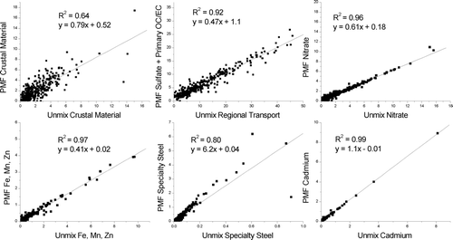
The R² values for all factors are reasonable and statistically significant, ranging from 0.64 for crustal material to 0.99 for the cadmium factor. The slope of the regression line, however, ranges from 0.41 for the Fe, Mn, and Zn factor to 6.2 for the specialty steel factor. The crustal material and the cadmium factors are within 20% in source contribution magnitude, suggesting that results are robust for these factors. PMF apportions more mass to the specialty steel factor due to the inclusion of 2% of the sulfate mass. PMF apportions less mass to the sulfate and primary OC and EC factors, the nitrate factor, and the Fe, Mn, and Zn factor. The apportionment of less mass to the sulfate and primary OC and EC factors by PMF as compared to the Unmix regional transport factor is likely due to Unmix fitting the model to total PM_2.5, while PMF has a significant fraction of unexplained mass. For the nitrate and Fe, Zn, and Mn factors, the difference is due to the apportionment of OC and EC. Unmix apportions 17% of the OC mass and 17% of the EC mass to the nitrate factor whereas PMF apportions 7% OC mass and 5% EC mass to the nitrate factor. For the Fe, Mn, and Zn factor, the apportionment is 12% of the OC mass and 18% of the EC mass explained by Unmix, but only 4% of the OC mass and 7% of the EC mass is explained by the same PMF factor. Results from previous comparisons of PMF and Unmix show similar conclusions: convergence for some factors but poor agreement for others (Poirot et al. 2001; Maykut et al. 2003).

In comparing Figure 3 and Figure 5, the average source contributions as a percent of average PM_2.5 mass are within a few percent for the two models for all factors, with the exception of the Unmix regional transport factor (68%) and the sulfate and primary OC and EC factor for PMF (total 40%). Unmix apportions all the mass, while on average PMF apportions only 78% of the mass, so some discrepancy is expected. PMF is more effective at discerning between primary and secondary OC; Unmix does not distinguish between the two and therefore can only give a large factor that is general regionally transported material and is not very informative from a policy-making perspective.

Adding Individual Organic Markers into Model

In an effort to further identify the sources apportioned by PMF, selected species of OC were added to the dataset. Individual organic compounds have been used as markers for specific sources; for example, hopanes are good tracers for vehicle exhaust, both gasoline and diesel engines (Simoneit 1984; Rogge et al. 1993a; Schauer et al. 1996). Organic molecular markers have been identified through a combination of source testing and analysis of ambient data (see, e.g., Rogge et al. 1996; Schauer et al. 1996; Simoneit 1999, 2002 and references therein). Table 2 lists the organic species included in the PMF model and their major sources (Rogge et al. 1996; Schauer et al. 1996; Robinson et al. 2006a, b, c; Subramanian et al. 2005a, b). These are the set of species most commonly used for chemical mass balance modeling of sources of primary organic aerosol (Schauer et al. 1996; Watson et al. 1998; Schauer and Cass 2000; Schauer et al. 2002a; Zheng et al. 2002; Fraser et al. 2003; Robinson et al. 2006a, b, c; Subramanian et al. 2005a, b). Adding these compounds presents a new level of difficulty, however, since compounds can experience transformations during transport from source to receptor. Schauer et al. (1996) and Rogge et al. (1996) examined issues associated with chemical stability and classified certain compounds as stable in the context of Los Angeles. Here, as in previous source apportionment analysis using molecular markers, we assume that mass is conserved and the chemical transformation of tracer species during transport to the receptor site is minimal. Robinson et al. (2005) examines the Pittsburgh data set for evidence of photochemical oxidation of molecular markers.

TABLE 2 Species of organic carbon that are included in the PMF model. The abbreviations in all capital letters correspond to the x-axis labels in Figure 7

Compound (abbreviation)	Sources	References
n-Nonacosane (NAL09)	Vegetative detritus, road-dust, tire wear	(Simoneit and Mazurek 1982, Rogge et al. 1993b, 1993c)
n-Triacontane (NAL10)	Vegetative detritus, road-dust, tire wear	(Simoneit and Mazurek 1982; Rogge et al. 1993b, 1993c)
n-Hentriacontane (NAL11)	Vegetative detritus, road-dust, tire wear	(Simoneit and Mazurek 1982; Rogge et al. 1993b, 1993c)
n-Dotriacontane (NAL12)	Vegetative detritus, road-dust, tire wear	(Simoneit and Mazurek 1982; Rogge et al. 1993b, 1993c)
n-Tritriacontane (NAL13)	Vegetative detritus, road-dust, tire wear	(Simoneit and Mazurek 1982; Rogge et al. 1993b, 1993c)
Hexadecanoic acid (palmitic acid) (NACD6)	Cooking	(Rogge et al. 1991; Schauer et al. 1999, 2002b)
Octadecanoic acid (stearic acid) (NACD8)	Cooking	(Rogge et al. 1991; Schauer et al. 1999, 2002b)
Pimaric acid, Sandaracopimaric acid, Dehydroabietic acid, and 7-Oxodehydroabietic acid (RSNSM)	Softwood combustion	(Rogge et al. 1998; Simoneit 2002)
Syringaldehyde (SYALD)	Hardwood combustion	(Rogge et al. 1998; Simoneit 2002)
Acetosyringone (ACSYN)	Hardwood combustion	(Rogge et al. 1998; Simoneit 2002)
Syringic Acid (SYNCD)	Hardwood combustion	(Rogge et al. 1998; Simoneit 2002)
Levoglucosan (LEVOG)	Wood combustion (both types)	(Simoneit et al. 1999)
22,29,30-Trisnorneohopane (HOP1)	Vehicular exhaust	(Simoneit 1985; Rogge et al. 1993a)
17@(H),21A(H)-29-Norhopane (HOP2)	Vehicular exhaust	(Simoneit 1985; Rogge et al. 1993a)
17@(H),21A(H)-Hopane (HOP3)	Vehicular exhaust	(Simoneit 1985; Rogge et al. 1993a)
22S+R-17@(H),21A(H)−30-Homohopane (HOP4,5)	Vehicular exhaust	(Simoneit 1985; Rogge et al. 1993a)
22S+R-17@(H),21A(H)-30-Bishomohopane (HOP6,7)	Vehicular exhaust	(Simoneit 1985; Rogge et al. 1993a)
Benzo(e)pyrene (BNZEP)	For Pittsburgh, mainly: Vehicular exhaust, wood combustion, coke-production	(Simoneit 1985; Rogge et al. 1993a; Schauer and Cass 2000; Robinson et al. 2006a, b, c; Subramanian et al. 2005a, b)
Indeno[1,2,3-cd]pyrene (INDCDP)	For Pittsburgh, mainly: Vehicular exhaust, wood combustion, coke-production	(Simoneit 1985; Rogge et al. 1993a; Schauer and Cass 2000; Robinson et al. 2006a, b, c; Subramanian et al. 2005a, b)
Benzo[g,h,i]perylene (BNZGHI)	For Pittsburgh, mainly: Vehicular exhaust, wood combustion, coke-production	(Simoneit 1985; Rogge et al. 1993a; Schauer and Cass 2000; Robinson et al. 2006a, b, c; Subramanian et al. 2005a, b)
Coronene (CORON)	For Pittsburgh, mainly: Vehicular exhaust, wood combustion, coke-production	(Simoneit 1985; Rogge et al. 1993a; Schauer and Cass 2000; Robinson et al. 2006a, b, c; Subramanian et al. 2005a, b)
Benzo(b+j+k)fluoranthenes (BNBJKF)	For Pittsburgh, mainly: Vehicular exhaust, wood combustion, coke-production	(Simoneit 1985; Rogge et al. 1993a; Schauer and Cass 2000; Robinson et al. 2006a, b, c; Subramanian et al. 2005a, b)

For organic compound speciation of PM_2.5, a total of 133 samples, including field handling blanks, were collected using a PM_2.5 sampler (Tisch Environmental, Inc. Model TE-1000 PUF) equipped with an URG cyclone (URG-2000-30AE, URG Corp.) to remove particles with an aerodynamic diameter larger than 2.5 μ m. The particulate matter was collected on a sampling module consisting of a quartz fiber filter (102 mm diameter, Pall Lifesciences, Tissuquartz 2500 QAT-UP) followed by a polyurethane foam (PUF) plug (7.5 cm long, Tisch Environmental, Inc. TE-1010) installed downstream of the filter to trap semi-volatile organic compounds that are associated with particulate matter and volatilize off the filter during the sampling process. The sampler was operated at 145 lpm. Samples were collected for 24-hour periods starting at midnight daily during July 2001 and several days in January 2002, and every sixth day during the baseline study (August 12 to December 26, 2001; January 29 to July 1, 2002). Details of the quartz and PUF plug preparation and the subsequent GC/MS analysis and ambient concentrations of individual organic compounds are reported by Bernardo-Bricker et al. (2005). While the trace element, sulfate, nitrate, OC and EC data are available as daily 24-hour averages for a total of 386 days, the speciated OC sampling and analysis occurred on a more intermittent schedule, with 24-hour averages for a total of only 97 days. However, PMF is capable of providing reasonable results for datasets containing elements with as much as 27–98% of the data missing or below the detection limit (Polissar et al. 2001; Polissar et al. 1998). As with the other species, missing data for the OC species were replaced by the geometric mean concentration and assigned an uncertainty of four times that average. The missing data were assumed to have sufficiently high uncertainty so as not to give weight to the model results.

In including the speciated OC data in the PMF model, groups of similar species, such as the hopanes, were added individually to determine the effect on the model results. With positive results, more species were added and many combinations were tested until an optimum solution was reached. Some species showed very strong correlations with existing PMF-modeled factors. All of the hopane species showed strong correlation with the primary OC and EC factor, further reinforcing the assumption that this factor is related to vehicle emissions. Some species did not add any new information to the model as they did not correlate with any of the 10 existing factors, or did not form a new factor. The cigarette smoke tracers and some food cooking tracers are examples of this situation and therefore they were not included in the model. It is possible that these sources are relatively small as compared to the other identified factors and therefore could not be identified by PMF. It is also possible that with so much missing data, the quality of the data is insufficient to form a recognizable source signature.

The best solution is presented in Figure 7, Figure 8, Figure 9. PMF determined 11 factors in a result that is similar to the solution described by Figure 1, Figure 2, and Figure 5, but with one factor changing significantly. This is the primary OC and EC factor, which has split into two different factors, one associated with vehicles and road dust, and the other associated with wood combustion, cooking, and vegetative detritus. Although there are separate tracers for hardwood and softwood combustion, the model could not separate the two, and therefore the factor is termed “wood combustion.” The partitioning of the OC fraction in the secondary sulfate and nitrate factors changed slightly, with the fraction of OC in the sulfate factor decreasing from 19% to 5%, and the fraction of OC in the nitrate factor decreasing from 7% to 6%. This could suggest that adding the molecular markers to the PMF analysis enables further identification of primary sources in such a manner that the secondary contribution of OC is reduced. Because all other factors are approximately the same as shown in Figure 1, Figure 2, and Figure 5, Figure 7 and Figure 8 only show the results for the wood combustion, cooking, and vegetative detritus factor and the vehicle emissions and road dust factor. The theoretical Q value for this dataset was 17,370 and the actual Q value was 17,711. As was the case for the original solution, the result with speciated OC was not sensitive to rotation, but G-space plotting showed the best solution occurred with FPEAK of –0.2.

Figure 9 is consistent with Figure 5, showing a maximum 5% difference in study average contributions for comparable source categories. Note that the primary OC and EC factor in Figure 5 is now represented by two factors in Figure 9: (1) vehicles and road dust and (2) wood combustion, vegetative detritus, and cooking. These minor differences are mostly due to the distribution of OC and EC in the two models. For example, the OC fraction in the sulfate source went from 25% in the first PMF solution to 19% in the solution that includes molecular markers.

FIG. 7 PMF with speciated OC source composition for the wood combustion, vegetative detritus and cooking factor and the vehicle emissions and road dust factor.

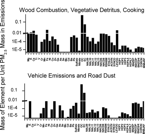
FIG. 8 PMF with speciated OC source contribution for the wood combustion, vegetative detritus and cooking factor and the vehicle emissions and road dust factor.

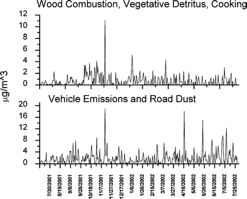
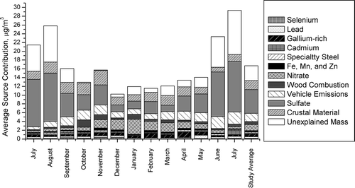
FIG. 9 Monthly average PMF source contributions for the PMF solution containing molecular markers. Height of the bars corresponds to the monthly average PM_2.5 mass measured with a TEOM. The study average represents the average source contributions from July 11, 2001 through July 31, 2002. The unexplained mass is the difference between the monthly average PM_2.5 mass and the sum of the monthly averaged source contributions from each factor.

Vehicles and Road Dust Factor

This factor accounts for 11% of the PM_2.5 mass and is primarily composed of 86% OC and 11% EC. OC, EC, hopanes, PAH's, and n-alkanes are important components of this factor. For OC, EC, hopanes, and PAH's, correlations between species concentrations and source contributions were 0.6 or greater, while the correlations for the larger n-alkanes were 0.4–0.5. These compounds are molecular markers for motor vehicle exhaust (Simoneit 1985; Rogge et al. 1993a, b, c; Simoneit and Mazurek 1982; Schauer and Cass 2000; Robinson et al. 2006a, b, c; Subramanian et al. 2005a, b). The lower correlation for the n-alkanes, less than the 0.7 desired, is likely due to the fact that they are present in emissions from many sources and not just motor vehicles. But their appearance as markers for this factor suggests that a fraction of the larger n-alkanes is attributed to road dust that is redistributed by vehicular traffic. It is assumed that the fraction of the larger n-alkanes in vegetative detritus would be better correlated with wood combustion. No seasonal trend is observed for this factor.

Wood Combustion, Vegetative Detritus and Cooking Factor

Levoglucosan, resin acids, syringols, stearic acid, palmitic acid, and the n-alkanes are important markers for this factor, composed of 75% OC, 11% EC, 3% Levoglucosan, 3% Ca, 3% Fe, and 2% K. These compounds, as listed in Table 2, are markers of wood smoke, vegetative detritus, and cooking and therefore this factor is labeled as a composite of these three sources. Correlations of these species concentrations with source contributions are between 0.5–0.6, with the exception of stearic acid (0.3). The source contribution is highest during the autumn months of October and November, presumably from residential wood burning. Although PAH's can also be markers of wood smoke, these species do not correlate well with this factor, suggesting that PAH emissions in the Pittsburgh region are dominated by other sources listed in Table 2, such as coke production and vehicle exhaust (Robinson et al. 2006a, b, c). Potassium is often considered to be a tracer of biomass combustion. Although there is a significant amount of potassium in this factor (2%), the correlation is low and it is therefore not considered a tracer here.

CONCLUSIONS

With the application of the Unmix and PMF models to the data collected during the PAQS, the contributions of a broad range of sources to the local airborne particles in the region have been determined. Comparison of the two models shows similar source composition and contribution for five factors: crustal material, nitrate, an Fe, Mn, and Zn factor, specialty steel production, and a cadmium factor. PMF found several additional factors: a gallium-rich factor, a lead factor, and a selenium factor assumed to be related to coal combustion. The PMF model found a sulfate factor separate from the OC and EC associated with primary emissions, while Unmix grouped these three species together into a single factor. Comparison between source contributions for the similar factors shows reasonable agreement between the two models. The sulfate factor shows the highest contribution to local PM_2.5 with an annual average contribution of approximately 28% (from PMF). The nitrate, crustal material, and primary OC and EC factors also show significant contributions on the order of 10–14%. The sulfate factor is affected by photochemistry and therefore shows maximum values in summer. The nitrate factor is temperature sensitive due to the volatility of nitrate; maximum values of particulate nitrate occur in winter. The crustal material and vehicle sources somewhat more constant contributions throughout the year. The remaining factors contribute on a smaller scale and are defined by plume events, with peaks in concentration distinctly higher than average concentration.

Adding speciated OC to the existing PMF model separates the primary OC and EC into two factors: vehicle emissions and road dust, and wood combustion, vegetative detritus and cooking. The hopanes, PAH's, and wood smoke tracers, despite a large percentage of missing data, showed good correlations with their respective factors, illustrating the power of PMF to accommodate datasets with large quantities of missing data. The wood combustion, cooking, and vegetative detritus factor contributes a small amount to ambient PM_2.5 in Pittsburgh, approximately 4%. There were several molecular markers considered or used in the model that did not yield a resolved factor based on the source of the molecular marker in Table 2. Meat cooking and cigarette smoking factors were not resolved, and distinctions between hardwood and softwood combustion factors were not made. Some molecular markers may prove better tracers than others and therefore the lack of further resolution of factors may be due to the large amount of missing data.

A future paper will discuss identifying the locations of sources of the observed species, Pekney et al. (2005). The conditional probability function (CPF) and the potential source contribution function (PSCF) will use the modeled source contributions and wind direction data or back trajectories to find most probable location of the sources.

This research was conducted as a part of the Pittsburgh Air Quality Study which was supported by the US Environmental Protection Agency under contract R82806101 and the US Department of Energy National Energy Technology Laboratory under contract DE-FC26-01NT41017. This paper has not been subject to EPA's peer and policy review, and therefore does not necessarily reflect the views of the Agency. No official endorsement should be inferred.

REFERENCES

- American Iron and Steel Institute (AISI) . 2004 . http://www.steel.org
- Anderson , R. , Martello , D. , White , C. , Crist , K. , John , K. , Modey , W. and Eatough , D. J. 2004 . The Regional Nature of PM2.5 Episodes in the Upper Ohio River Valley . J. Air & Waste Manage. Assoc. , 54 : 971 – 984 . [CSA]
- Bautista , R. G. 2003 . Processing to Obtain High-Purity Gallium . JOM. , 55 : 23 – 26 . [CSA]
- Bernardo-Bricker , A. and Rogge , W. 2005 . Ambient Organic PM2.5 at the Pittsburgh Air Quality Study: Seasonal Variations and Regional Contributions . Atmospheric Environment , [CSA]
- Cabada , J. C. , Khlystov , A. , Wittig , E. , Pilinis , C. and Pandis , S. 2004 . Light Scattering by Fine Particles During the Pittsburgh Air Quality Study: Measurements and Modeling . J. Geophys. Res. , 109 : D16S03 [CROSSREF] [CSA]
- Cabada , J. C. , Pandis , S. N. and Robinson , A. L. 2002 . Sources of Atmospheric Carbonaceous Particulate Matter in Pittsburgh, Pennsylvania . J. Air & Waste Manage. Assoc. , 52 : 732 – 741 . [CSA]
- Dockery , D. W. , Pope , C. A. , Xu , X. P. , Spengler , J. D. , Ware , J. H. , Fay , M. E. and Ferris , B. G. 1993 . An Association Between Air Pollution and Mortality in Six United States Cities . New Engl. J. Med. , 329 : 1753 – 1759 . [INFOTRIEVE] [CROSSREF] [CSA]
- Eatough , D. J. , Modey , W. K. , Mangelson , N. F. , Anderson , R. R. and Martello , D. V. 2005 . Apportionment of Ambient Primary and Secondary PM2.5 During a 2001 Summer Study in the NETL Pittsburgh Site Using PMF2 and EPA UNMIX . Aerosol Sci. Technol. , in press[CSA]
- Fraser , M. P. , Yue , Z. W. and Buzcu , B. 2003 . Source Apportionment of Fine Particulate Matter in Houston, TX, Using Organic Molecular Markers . Atmos. Environ. , 37 : 2117 – 2123 . [CROSSREF] [CSA]
- Henry , R. C. 1997 . History and Fundamentals of Multivariate Air Quality Models . Chemometrics and Intelligent Laboratory Systems , 37 : 37 – 42 . [CROSSREF] [CSA]
- Henry , R. C. 2001 . Unmix Version 2.4 Manual. Available with Unmix software [email protected]
- Henry , R. C. Personal communication
- Kim , E. , Hopke , P. K. and Edgerton , E. 2003 . Source Identification of Atlanta Aerosol by Positive Matrix Factorization . J. Air & Waste Manage. Assoc. , 53 : 731 – 739 . [CSA]
- Kim , E. , Hopke , P. K. , Larson , T. V. and Covert , D. S. 2004 . Analysis of Ambient Particle Size Distributions using Unmix and Positive Matrix Factorization . Environ. Sci. Technol. , 38 : 202 – 209 . [INFOTRIEVE] [CROSSREF] [CSA]
- Larsen , R. K. and Baker , J. E. 2003 . Source Apportionment of Polycyclic Aromatic Hydrocarbons in the Urban Atmosphere: A Comparison of Three Methods . Environ. Sci. Technol. , 37 : 1873 – 1881 . [INFOTRIEVE] [CROSSREF] [CSA]
- Lithgow , G. , Robinson , A. and Buckley , S. 2004 . Ambient Measurements of Metal-Containing PM2.5 in an Urban Environment Using Laser-Induced Breakdown Spectroscopy . Atmos. Environ. , 38 : 3319 – 3328 . [CROSSREF] [CSA]
- Maykut , N. , Lewtas , J. , Kim , E. and Larson , T. 2003 . Source Apportionment of PM2.5 at an Urban IMPROVE Site in Seattle, Washington . Environ. Sci. Technol. , 37 : 5135 – 5142 . [INFOTRIEVE] [CROSSREF] [CSA]
- Modey , W. , Eatough , D. J. , Anderson , R. , Martello , D. , Takahama , S. , Lucas , L. and Davidson , C. I. 2005 . Apportionment of Ambient Primary and Secondary Pollutants During a 2001 Summer Study in Pittsburgh Using EPA UNMIX . J. of the Air & Waste Manage. Assoc. , Submitted[CSA]
- NIOSH . 1996 . “ Elemental Carbon (Diesel Exhaust) ” . In NIOSH Manual of Analytical Methods , Cincinnati, OH : National Institute of Occupational Safety and Health .
- Olmez , I. , Sheffield , A. , Gordon , G. , Houck , J. , Pritchett , L. , Cooper , J. , Dzubay , T. and Bennett , R. 1998 . Compositions of Particles from Selected Sources in Philadelphia for Receptor Modeling Applications . JAPCA. , 38 : 1392 – 1402 . [CSA]
- Paatero , P. and Tapper , U. 1993 . Analysis of Different Modes of Factor Analysis as Least Square Fit Problems . Chemometrics and Intelligent Laboratory Systems. , 18 : 183 – 194 . [CROSSREF] [CSA]
- Paatero , P. and Tapper , U. 1994 . Positive Matrix Factorization: A Non-Negative Factor Model with Optimal Utilization of Error Estimates of Data Values . Environmetrics. , 5 : 111 – 126 . [CSA]
- Paatero , P. 1997 . Least Squares Formulation of Robust Non-Negative Factor Analysis . Chemometrics and Intelligent Laboratory Systems. , 37 : 15 – 35 . [CROSSREF] [CSA]
- Paatero , P. , Hopke , P. K. , Begum , B. A. and Biswas , S. K. 2005 . A Graphical Diagnostic Method for Assessing the Rotation in Factor Analytical Models of Atmospheric Pollution . Atmos. Environ. , 39 : 193 – 201 . [CROSSREF] [CSA]
- Parekh , P. 1990 . Study of Manganese from Anthropogenic Emissions at a Rural Site in the Eastern United States . Atmos. Environ. , 24A : 415 – 421 . [CSA]
- Pekney , N. J. and Davidson , C. I. 2005 . Determination of Trace Elements in Ambient Aerosol Samples . Analytica Chimica Acta. , 540 : 269 – 277 . [CROSSREF] [CSA]
- Pekney , N. J. , Davidson , C. I. , Zhou , L. and Hopke , P. K. 2005 . Application of PSCF and CPF to PMF-Modeled Sources of PM2.5 in Pittsburgh . Aerosol Sci. & Technol. , in press[CSA]
- Poirot , R. L. , Wishinski , P. R. , Hopke , P. K. and Polisar , A. V. 2001 . Comparative Application of Multiple Receptor Methods to Identify Aerosol Sources in Northern Vermont . Environ. Sci. Technol. , 35 : 4622 – 4636 . [INFOTRIEVE] [CROSSREF] [CSA]
- Polidori , A. , Turpin , B. , Lim , H. , Totten , L. and Davidson , C. 2005 . Polarity and Molecular Weight/Carbon Weight of the Pittsburgh Organic Aerosol Manuscript in preparation
- Polissar , A. V. , Hopke , P. K. , Malm , W. C. and Sisler , J. F. 1998 . Atmospheric Aerosol over Alaska: 2. Elemental Composition and Sources . J. Geophys. Res. , 103 : 19,045 – 19,057 . [CSA]
- Polissar , A. V. , Hopke , P. K. and Poirot , R. L. 2001 . Atmospheric Aerosol over Vermont: Chemical Composition and Sources . Environ. Sci. Technol. , 35 : 4604 – 4621 . [INFOTRIEVE] [CROSSREF] [CSA]
- Pope , C. A. , Burnett , R. T. , Thun , M. J. , Calle , E. E. , Krewski , D. , Ito , K. and Thurston , G. D. 2002 . Lung Cancer, Cardiopulmonary Mortality and Long-Term Exposure to Fine Particulate Air Pollution . JAMA , 287 : 1132 – 1141 . [INFOTRIEVE] [CROSSREF] [CSA]
- Rees , S. L. , Robinson , A. L. , Khylstov , A. , Stanier , C. O. and Pandis , S. 2004 . Mass Balance Closure and the Federal Reference Method for PM2.5 in Pittsburgh, Pennsylvania . Atmos. Environ. , 38 : 3305 – 3318 . [CROSSREF] [CSA]
- Robinson , A. L. , Donahue , N. M. and Rogge , W. F. 2005 . Photochemical Oxidation and Changes in Molecular Composition of Organic Aerosol in the Regional Context . J. Geophys. Res.-Atmos. , Submitted[CSA]
- Robinson , A. L. , Subramanian , R. , Donahue , N. M. , Bernardo-Bricker , A. and Rogge , W. F. 2006a . Source Apportionment of Molecular Markers and Organic Aerosol—1. Methodology for Visually Comparing Source Profiles and Ambient Data . Environ. Sci. Technol. , Submitted[CSA]
- Robinson , A. L. , Subramanian , R. , Donahue , N. M. , Bernardo-Bricker , A. and Rogge , W. F. 2006b . Source Apportionment of Ambient Organic Aerosol—2. Biomass Smoke . Environ. Sci. Technol. , Submitted[CSA]
- Robinson , A. L. , Subramanian , R. , Donahue , N. M. , Bernardo-Bricker , A. and Rogge , W. F. 2006c . Source Apportionment of Ambient Organic Aerosol—3. Food Cooking Emissions . Environ. Sci. Technol. , Submitted[CSA]
- Rogge , W. F. , Hildemann , L. M. , Mazurek , M. A. , Cass , G. R. and Simoneit , B. R. T. 1993a . Sources of Fine Organic Aerosol 2. Noncatalyst and Catalyst-Equipped Automobiles and Heavy-Duty Diesel Trucks . Environ. Sci. Technol. , 27 : 636 – 651 . [CROSSREF] [CSA]
- Rogge , W. F. , Hildemann , L. M. , Mazurek , M. A. , Cass , G. R. and Simoneit , B. R. T. 1993b . Sources of Fine Organic Aerosol .3. Road Dust, Tire Debris, and Organometallic Brake Lining Dust—Roads as Sources and Sinks . Environ. Sci. Technol. , 27 : 1892 – 1904 . [CROSSREF] [CSA]
- Rogge , W. F. , Hildemann , L. M. , Mazurek , M. A. , Cass , G. R. and Simoneit , B. R. T. 1993c . Sources of Fine Organic Aerosol .4. Particulate Abrasion Products from Leaf Surfaces of Urban Plants . Environ. Sci. Technol. , 27 : 2700 – 2711 . [CROSSREF] [CSA]
- Rogge , W. F. , Hildemann , L. M. , Mazurek , M. A. , Cass , G. R. and Simoneit , B. R. T. 1996 . Mathematical Modeling of Atmospheric Fine Particle-Associated Primary Organic Compound Concentrations . J. Geophys. Res.-Atmospheres. , 101 ( D14 ) : 19379 – 19394 . [CROSSREF] [CSA]
- Rogge , W. F. , Hildemann , L. M. , Mazurek , M. A. , Cass , G. R. and Simonelt , B. R. T. 1991 . Sources of Fine Organic Aerosol .1. Charbroilers and Meat Cooking Operations . Environ. Sci. Technol. , 25 : 1112 – 1125 . [CROSSREF] [CSA]
- Schauer , J. J. and Cass , G. R. 2000 . Source Apportionment of Wintertime Gas-Phase and Particle-Phase air Pollutants Using Organic Compounds as Tracers . Environ. Sci. Technol. , 34 : 1821 – 1832 . [CROSSREF] [CSA]
- Schauer , J. J. , Fraser , M. P. , Cass , G. R. and Simoneit , B. R. T. 2002a . Source Reconciliation of Atmospheric Gas-Phase and Particle-Phase Pollutants During a Severe Photochemical Smog Episode . Environ. Sci. Technol. , 36 : 3806 – 3814 . [INFOTRIEVE] [CROSSREF] [CSA]
- Schauer , J. J. , Kleeman , M. J. , Cass , G. R. and Simoneit , B. R. T. 2002b . Measurement of Emissions from Air Pollution Sources. 4. C-1-C-27 Organic Compounds from Cooking with Seed Oils . Environ. Sci. Technol. , 36 : 567 – 575 . [INFOTRIEVE] [CROSSREF] [CSA]
- Schauer , J. J. , Kleeman , M. J. , Cass , G. R. and Simoneit , B. R. T. 1999 . Measurement of Emissions from Air Pollution Sources. 1. C-1 Through C-29 Organic Compounds from Meat Charbroiling . Environ. Sci. Technol. , 33 : 1566 – 1577 . [CROSSREF] [CSA]
- Schauer , J. J. , Rogge , W. F. , Hildemann , L. M. , Mazurek , M. A. and Cass , G. R. 1996 . Source Apportionment of Airborne Particulate Matter Using Organic Compounds as Tracers . Atmos. Environ. , 30 : 3837 – 3855 . [CROSSREF] [CSA]
- Simoneit , B. R. T. 1984 . Organic-Matter of the Troposphere. 3. Characterization and Sources of Petroleum and Pyrogenic Residues in Aerosols over the Western United-States . Atmos. Environ. , 18 : 51 – 67 . [CROSSREF] [CSA]
- Simoneit , B. R. T. 1985 . Application of Molecular Marker Analysis to Vehicular Exhaust for Source Reconciliations . Int. J. Environ. Anal. Chem. , 22 : 203 – 233 . [CSA]
- Simoneit , B. R. T. 1999 . A Review of Biomarker Compounds as Source Indicators and Tracers for Air Pollution . Environ. Sci. Pollution Res. , 6 : 159 – 169 . [CSA]
- Simoneit , B. R. T. 2002 . Biomass Burning—A Review of Organic Tracers for Smoke from Incomplete Combustion . Appl. Geochem. , 17 : 129 – 162 . [CROSSREF] [CSA]
- Simoneit , B. R. T. and Mazurek , M. A. 1982 . Organic-Matter of the Troposphere. 2. Natural Background of Biogenic Lipid Matter in Aerosols over the Rural Western United-States . Atmos. Environ. , 16 : 2139 – 2159 . [CROSSREF] [CSA]
- Simoneit , B. R. T. , Schauer , J. J. , Nolte , C. G. , Oros , D. R. , Elias , V. O. , Fraser , M. P. , Rogge , W. F. and Cass , G. R. 1999 . Levoglucosan, A Tracer for Cellulose in Biomass Burning and Atmospheric Particles . Atmos. Environ. , 33 : 173 – 182 . [CROSSREF] [CSA]
- Subramanian , R. , Robinson , A. L. , Donahue , N. M. , Bernardo-Bricker , A. and Rogge , W. F. 2005a . Source Apportionment of Gasoline and Diesel Vehicles using the Chemical Mass Balance Model and Molecular Markers . Atmos. Environ. , Submitted[CSA]
- Subramanian , R. , Donahue , N. M. , Bernardo-Bricker , A. , Rogge , W. F. and Robinson , A. L. 2005b . Source Apportionment of Primary Organic Aerosol in Pittsburgh, PA Using Organic Molecular Markers . Atmos. Environ. , Manuscript in preparation, [CSA]
- Subramanian , R. 2004 . Sampling, Analysis, and Source-Apportionment of Ambient Carbonaceous Aerosols , Ph.D Dissertation Pittsburgh, PA : Carnegie Mellon University .
- Subramanian , R. , Khlystov , A. Y. , Cabada , J. C. and Robinson , A. L. 2004 . Positive and Negative Artifacts in Particulate Organic Carbon Measurements with Denuded and Undenuded Sampler Configurations . Aerosol Sci. Technol. , 38 ( S1 ) : 27 – 48 . [CSA]
- Takahama , S. , Wittig , B. , Vayenas , D. , Davidson , C. and Pandis , S. N. 2004 . Modeling the Diurnal Variation of Nitrate During the Pittsburgh Air Quality Study . J. Geophys. Res.—Atmos. , 109 ( D16 ) Art. No. D16S06[CSA]
- Tang , W. , Raymond , T. , Wittig , B. , Davidson , C. I. , Pandis , S. N. , Robinson , A. L. and Crist , K. 2004 . Spatial Variations in PM2.5 During the Pittsburgh Air Quality Study . Aerosol Sci. Technol. , 38 ( S2 ) : 80 – 90 . [CROSSREF] [CSA]
- Turpin , B. and Lim , H. 2001 . Species Contributions to PM2.5 Mass Concentrations: Revisiting Common Assumptions for Estimating Organic Mass . Aerosol Sci. Technol. , 35 : 602 – 610 . [CSA]
- U.S. Department of Energy . 2002 . Energy Information Administration . State Electricity Profiles , http://www.eia.doe.gov/cneaf/electricity/st_profiles/pennsylvania.pdf. Accessed 2004[CSA]
- U.S. Environmental Protection Agency . 1997a . National Ambient Air Quality Standards for Particulate Matter—Final Rule, 40 CFR part 50 . Federal Register , 62 ( 138 ) : 38 651–38,760, July 18[CSA]
- U.S. Environmental Protection Agency . 1997b . Compendium of Methods for the Determination of Inorganic Compounds in Ambient Air EPA/625/R-96/010a. January 1997
- U.S. Environmental Protection Agency . 2002 . “ Toxics Release Inventory Explorer version 4.3 ” . http://www.epa.gov/triexplorer. Accessed 2004
- Watson , J. G. , Fujita , E. M. , Chow , J. C. and Zielinska , B. 1998 . “ Northern Front Range Air Quality Study Final Report and Supplemental Volumes ” . http://www.nfraqs.colostate.edu/nfraqs/index2.html. Accessed 2006
- Watson , J. , Chow , J. and Houck , J. 2001 . PM2.5 Chemical Source Profiles for Vehicle Exhaust, Vegetative Burning, Geological Material, and Coal Burning in Northwestern Colorado During 1995 . Chemosphere. , 43 : 1141 – 1151 . [INFOTRIEVE] [CROSSREF] [CSA]
- Wittig , A. E. , Anderson , N. J. , Khlystov , A. Y. , Pandis , S. N. , Davidson , C. I. and Robinson , A. L. 2004 . Pittsburgh Air Quality Study Overview . Atmos. Environ. , 38 : 3107 – 3125 . [CROSSREF] [CSA]
- Zheng , M. , Cass , G. R. , Shauer , J. J. and Edgerton , E. S. 2002 . Source Apportionment of PM2.5 in the Southeastern United States Using Solvent-Extractable Organic Compounds as Tracers . Environ. Sci. Technol. , 36 : 2361 – 2371 . [INFOTRIEVE] [CROSSREF] [CSA]
- Zhou , L. , Hopke , P. K. , Paatero , P. , Ondov , J. , Pekney , N. and Davidson , C. I. 2004 . Advanced Factor Analysis for Multiple Time Resolution Aerosol Composition Data . Atmos. Environ. , 38 : 4909 – 4920 . [CROSSREF] [CSA]