A Numerical Study of Calm Air Sampling with a Blunt Sampler

The performance of an idealized spherical sampler facing both vertically upwards and downwards in calm air is studied numerically. To describe the air flow around the sampler, both potential and viscous flow models have been adopted. The equations of particle motion are then solved to calculate the aspiration efficiency. The dependence of the aspiration efficiency upon the various parameters of importance in calm air sampling are investigated and compared where possible with the experimental work of Su and Vincent (2003, 2004a, b).

It is found that in the case of upwards sampling the bluntness of the sampler only has a significant effect upon aspiration for large sampling velocities, values that would not generally be physically realistic. In the case of downwards sampling an important non-dimensional quantity, B ² R _C , is identified, where B represents the sampler bluntness and R _C represents the gravitational effects. This quantity determines the physical conditions for which aspiration will not occur and also the limiting values of the aspiration efficiency when aspiration does occur. In the case of low sampling velocities a difference is noted between experimental and numerical results for aspiration efficiency raising the need for more experimental data in this area. For both upwards and downwards sampling the semi-empirical models of Su and Vincent (2004b) have been modified to account for the information gained from the study. This is particularly important in the downwards sampling case where the modified model is found to agree particularly well with the results obtained.

INTRODUCTION

Aerosol samplers are widely used in present-day environmental and health studies to measure the aerosol concentration in the air. However, due to the inertia of the particles moving in the air flow in the vicinity of the sampler, the measured aerosol concentration can differ from the real concentration. The distortion in the value of the concentration can be expressed by the aspiration efficiency, which is defined as the ratio of the measured and real aerosol concentrations. For historical reasons, attention has focussed on samplers operating in moving air where the wind speeds are such that the predominant force bringing particles into the vicinity of the sampler is the drag due to the air motion. Due to the numerous experimental and theoretical studies on this topic the performance of aerosol samplers in moving air is reasonably well understood. A review of much of this earlier work is given by Vincent (1989). However, the performance of samplers operating in calm, or near calm air, is less well understood and in the past has received less attention. This is a topic of importance as indoor air flows are usually characterized by very small velocities, see, Berry and Froude (1989) and Baldwin and Maynard (1998). For such conditions the model of calm air sampling is an accurate description of indoor aerosol sampling conditions.

Past experimental and theoretical studies of the aspiration efficiency for samplers operating in calm air include Davies and Peetz (1954), Kaslow and Emrich (1973, 1974), Yoshida et al. (1978), Belyaev and Kustov (1980), Agarwal and Liu (1980), Grinshpun et al. (1989), Chung and Dunn-Rankin (1993) and Dunnett (2002). Although these earlier works have increased our understanding of how samplers perform when operating in calm air conditions, our knowledge is far from complete. In particular the influence of the sampler body upon performance is not fully understood. Hence, in this work, a study is made of the performance of a blunt sampler operating in calm air. Recently experimental studies were undertaken into the sampling performance of thin-walled, and some simple blunt, samplers by Su and Vincent (2002, 2003, 2004a, 2004b). Such studies are invaluable in furthering our understanding on this topic as experimental data with which to validate numerical models is lacking due to the difficulties in obtaining it. In the case of the thin-walled samplers some numerical work was also undertaken by Su and Vincent (2004a). The experimental method, known as the direct method, involved the direct visual observation of the limiting particle trajectories and hence the results obtained do not include errors due to particle bounce or blow off from the external surface of the sampler. In the work of Su and Vincent, the experimental data is displayed in tabular form making it available to compare with numerical models. The experimental data for both the blunt and thin-walled samplers was used by Su and Vincent (2004b), to develop semi-empirical formula to describe the aspiration efficiency of samplers facing upwards, downwards and horizontally.

In this paper the results of numerical studies of the performance of a spherical sampler facing both vertically upwards and downwards in calm air are presented. In order to validate the models comparisons are made with the experimental data. The studies are based on three different incompressible fluid flow models: an analytical model of potential flow using point sinks, a potential flow model using the Boundary Element Method and a viscous flow model. The different flow models are compared in order to determine their possibilities for modelling the problem of calm air sampling with a blunt sampler.

PROBLEM FORMULATION

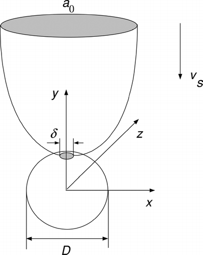
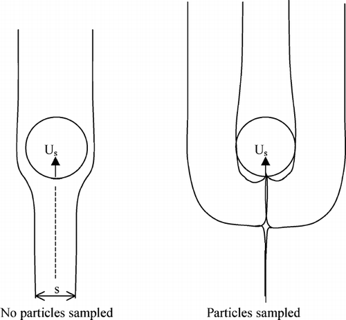
In order to compare with the available experimental data, a blunt spherical sampler with a single circular orifice orientated both vertically upwards and downwards is considered. The sampling orifice diameter δ is smaller than the sampling head diameter D. A schematic of the sampler is shown in Figure 1 for the case when it is orientated vertically upwards. The air is assumed to be stagnant far from the sampler and the particles move due to gravity in the negative y direction. Some of the falling particles are aspirated by suction through the sampling orifice. By tracing the particle paths it is possible to determine the limiting particle trajectory surface at a distance away from the sampler. This is the surface that separates the particles that are sampled from those that are not. An example of such a surface is also shown in Figure 1.

Figure 1 Schematic of sampler considered and limiting particle trajectory surface for the case when the sampler is oriented with the inlet pointing upwards.

The aspiration efficiency A is defined as the ratio of the concentration c of particles passing through the sampler inlet to that, c₀, in the undisturbed air far from the sampler. Using the continuity of particle fluxes inside the limiting particle trajectory surface we have

where v_s is the particle settling velocity, Q the sampling flow rate and a₀ is the horizontal area above the sampler enclosed by the limiting particle trajectory surface. Hence we can write the aspiration efficiency for the calm air sampling in the form

where U_S is the mean velocity across the plane of the sampling orifice.

If the sampler is pointing vertically upwards then a₀ is circular and is defined by its radius r₁. However when the sampler is pointing vertically downwards the sampler body blocks the falling particles. In this case a₀ is an annulus with inner radius r₂ and hence can be written as:

where r₁ and r₂ are the outer and inner radii of the area a₀ respectively. Hence the aspiration efficiency in the two cases considered here is given by:

where ′ denotes non-dimensional quantities, i.e. distances non-dimensionalised with respect to the sampler radius D/2, velocities with respect to sampling velocity U_s. The non-dimensional quantity B is the same as that used by Su and Vincent (2003) and is given by B = .

Hence determining A reduces to calculating the limiting particle trajectories by solving the equations of particle motion in a given velocity field.

FLOW MODELS

The equations of steady motion governing the air motion in sampling situations are the Navier-Stokes equations for incompressible flow which, in their non-dimensional form, are given by

The Reynolds number, Re = , where ν is the kinematic viscosity of the air, is a measure of the relative magnitudes of the inertial and viscous forces of the air.

In the work described here we have used three types of fluid flow models to describe the air flow in the sampler vicinity.

Potential Flow Models

If Re is very large then the viscous forces are negligible and inertial forces dominate. In this case the flow may be assumed to be inviscid and such an assumption greatly simplifies the equations of motion. In this work it has been assumed that the flow is inviscid and two potential models have been developed:

1.	A point sink model where the finite orifice on the sphere is modelled as the sum of a number N of point sinks. The model is described in detail in Galeev and Zaripov (2003). In the results shown here N = 91.
2.	A Boundary Element model where the flow velocities are obtained outside the sampler using the Boundary Element Method (BEM). The method in relation to calm air sampling problems has been described in detail in Dunnett and Wen (2002) and will not be repeated here.

For the sampling system considered Re is usually in the range O(10²)–O(10³) and although Re is large it is possible that within this range viscous effects become important. The inviscid case has been considered here in order to investigate its accuracy for modelling the sampling situation considered. A viscous flow model has also been adopted and results will be compared.

Viscous Flow Model

In this case a laminar flow model has been used to simulate the steady viscous flow for the spherical sampler. The control volume method and the SIMPLE algorithm (Patankar 1980) were employed in order to solve the equations for the air motion. As for the previous potential model, this method in relation to calm air sampling has been described in detail in Dunnett and Wen (2002) and hence is not repeated here.

PARTICLE MOTION

Once the velocity of the air has been obtained analytically or numerically, it is possible to trace the paths of the particles in the flow field. Neglecting the influence of the particles on the air flow, due to their small size and low concentrations, and all forces except the aerodynamic drag force and gravity, we can write the equations of particle motion in non-dimensional form as follows:

where u x ′, u_y′, u_z′ are the non-dimensional particle velocity components in the x′, y′, z′ directions respectively. The Stokes number St_C, representing the particle inertial effect, and the non-dimensional quantity R_C, representing the particle gravitational effect, are the same as those used by Su and Vincent (2003). Namely

where d_p and ρ are the diameter and density of the particle respectively, and μ is the dynamic viscosity of air. The drag coefficient C_D is a function of Re_p and in this work the expressions used are those given by Liu et al. (1989).

In tracing the particle paths the particles were started at a very large distance from the sampler, where the flow was assumed to be undisturbed by the physical presence of the sampler. It was assumed that the particles were then moving with the same velocity as the airflow plus their settling velocity, v_s, where

In the case when Re_p < 1, a condition often met in experiments, this becomes

The particles were then traced and the limiting particle trajectories, i.e., those separating the particles which pass through the sampling inlet from those that do not, were determined. In obtaining the limiting trajectories, it was assumed that any particle which impacted the sampler surface adhered to it and hence the only ones to enter the sampler were those that passed directly across the sampling inlet.

RESULTS

Flow Velocity Results

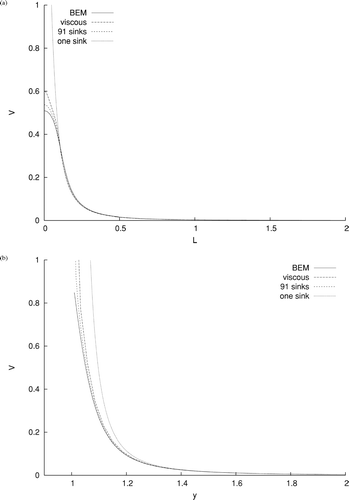
Initially a comparison was made between the flow velocities obtained by the three flow models described. An example of the results is shown in Figure 2 for B = 10. In Figure 2a the velocity along the axis orthogonal to the symmetry axis is shown as a function of the non-dimensional distance away from the symmetry axis, L. In Figure 2 y′ takes the value 1.05. In Figure 2b the velocity along the symmetry axis is shown as a function of the non-dimensional position along the axis. Also shown in the figures are the velocities obtained by modelling the sampling inlet by a single sink. It can be seen that the single sink is a reasonable model except in the region in the vicinity of the sampling inlet. It can also be seen from the figures that the agreement between the potential and viscous models is good.

Figure 2 The distribution of the magnitude of the non-dimensional air velocity, V, for the value of the bluntness parameter B = 10, (a) on the axis orthogonal to the symmetry axis at y′ = 1.05. L is the non-dimensional distance from the symmetry axis. (Sampling inlet at y′ ≈ 0.995); (b) along the symmetry axis. BEM denotes results obtained by the Boundary Element Method.

Sampler Pointing Upwards

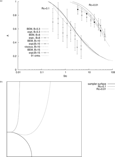
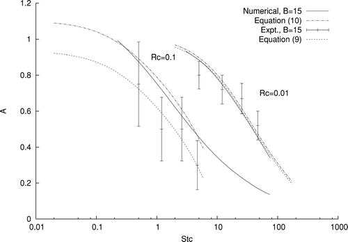
Considering the case where the sampler faces vertically upwards numerical results have initially been obtained to compare with the experimental data of Su and Vincent (2003). In the work of Su and Vincent (2003), results are published for two values of the gravitational parameter R_C, namely 0.1 and 0.01, for samplers such that B took values 5.3, 8, 10, and 15 and various values of the inertial parameter St_C. In Figure 3a, A is shown as a function of St_C for the two values of R_C considered by Su and Vincent (2003). For R_C = 0.1 results are shown for all three flow models described. However for R_C = 0.01 only the results from the BEM model and the viscous model are shown in the figure. This was done in order to make the figure clearer and because there was no discernable difference between the results obtained by the two potential models. As can be seen in Figure 3a all flow models give results that compare well with the experimental data. Although the numerical models do overestimate A in the majority of cases. The predictions of A obtained from the potential flow models, for the values of St_C considered experimentally, lie within experimental error for 50% of the cases. For the viscous flow model this percentage is increased with all results obtained by the model for the values of St_C considered experimentally, in the case of R_C = 0.01, lying within the experimental error bars. In general the viscous results do lie below the potential model results hence in some cases bringing them closer to the experimental range. This is expected as the viscous model is a more accurate description of the flow field in the vicinity of the sampler. It can be seen from the figure that the potential models more accurately predict the experimental results for the smaller value of R_C than they do for the larger values. For the range of conditions shown in Figure 3a a decrease in R_C is caused by an increase in sampling velocity U_S. As U_S increases it is expected that the error in the flow velocities predicted by the potential models due to the neglect of viscosity will not be so significant. This is what is observed here in Figure 3a. Also comparing the results obtained by the potential model for the two values of R_C considered, it can be seen that there is no significant difference in the results for the different values of B for R_C = 0.1 but there is for R_C = 0.01. In the case of R_C = 0.01 the limiting particle trajectories have to move up around the sampler body in order to enter the sampling inlet, see Figure 3b, which is not the case for R_C = 0.1, hence the bluntness of the sampler has more effect for the smaller R_C.

Figure 3 Results for the sampler pointing upwards to compare with the experimental data of Su and Vincent (2003). (a) Aspiration efficiency, A, as a function of Stokes number, St_C, for values of the gravitational parameter R_C = 0.1 and 0.01. BEM denotes results obtained by the Boundary Element Method. (b) limiting particle trajectories for Rc = 0.1 and Rc = 0.01 with bluntness parameter B = 5.3.

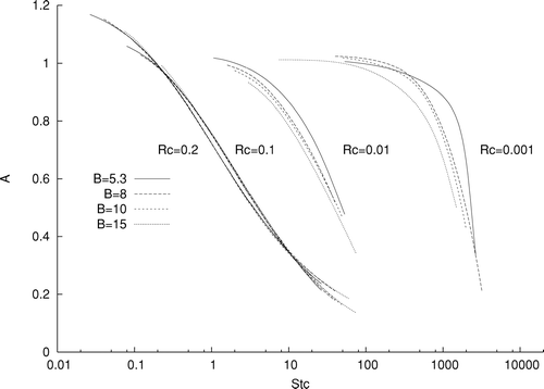
From Figure 3a we can see that although the viscous model is predicting the most accurate results, the potential models do predict values that are in reasonable agreement with the experimental data and the potential models are easier and less computationally expensive to obtain. Hence these models have been used to investigate the behaviour of A outside the range of values of R_C considered experimentally. It was found that the effect of the bluntness of the sampler upon performance became more significant as R_C decreased, though the effect was never great for parameter ranges corresponding to physically realistic situations. This is shown in Figure 4 where A is shown as a function of St_C for R_C = 0.2, 0.1, 0.01, and 0.001. The case of R_C = 0.001 corresponds to large particle sizes and high sampling velocities and is unlikely to occur physically, however it does give us an indication of how sampler bluntness effects change as R_C differs.

Figure 4 Aspiration efficiency, A, as a function of Stokes number, St_C, for values of the gravitational parameter R_C = 0.2, 0.1, 0.01, and 0.001 when the sampler is pointing upwards obtained numerically using the potential flow models.

Over the years attempts have been made to develop semi-empirical models of the aspiration efficiency of samplers. In the case of calm air sampling such models have been restricted by the lack of experimental data with which to validate them Grinshpun et al. (1993) explored a general equation for aspiration efficiency which could be applied to moving and calm air for a thin-walled sampler. In the case of calm air the model was restricted to a sampling orientation of 0 ≤ θ ≤ 90 where θ was the angle the sampler axis made with the vertical. As the model was developed for thin-walled samplers no account was taken for sampler bluntness. More recently, using their comprehensive experimental data, Su and Vincent (2004a) developed empirical formulae for thin-walled and blunt samplers operating in calm air. In the case of a blunt sampler pointing upwards the formula for A is given by:

where

This formula was derived using Levin's (1957) formula for a point sink model as a basis and hence is restricted to small values of the parameter k₁.

When the sampling velocity, U_S, is very low, leading to small St_C, particles may enter the sampling orifice directly by settling without help from the aspiration process. Hence in the limit St_C → 0, A → 1 + R_C. This behavior is independent of the shape of the sampler and hence will be true for thin-walled and blunt samplers. This has been noted previously by, for example, Yoshida et al. (1978) and Agarwal and Liu (1980) and was also found to be the case in the numerical results obtained here.

The experimental results of Su and Vincent (2003) do not appear to be tending to 1 + R_C as St_C becomes small, though if the error bars are taken into consideration it is possible. As noted by Su and Vincent (2003) such experiments are very difficult, and it is possible that for low sampling velocities where any air movement will be very slight, such difficulties are increased. Expression (9), which was developed using the experimental data, has the property that A → 1 − R_C ^3/2(B^1/2 − 1) as St_C → 0. Hence expression (9) will be inaccurate for small St_C and this inaccuracy will increase as R_C increases. Also, in expression (9), B has a greater effect on A as R_C increases. This is contrary to what has been observed here numerically.

An attempt has been made to modify Equation (9) in order to obtain the correct limiting behavior at small St_C. Using Equation (9) as the starting point and altering it to obtain A = 1 + R_C when St_C = 0 expression (10) has been obtained.

As for Equation (9), expression (10) is only valid for k₁ < 1, hence restricting it to the ranges St_C ≤ 8 for R_C = 0.1 and St_C ≤ 250 for R_C = 0.01. The numerical results do not have these restrictions. Equation (10) was found to model well the behavior of A for small k₁, see Figure 5 where the expression is shown for R_C = 0.1 and 0.01. Only one value of B is shown when displaying the numerical results in order to make the figure clearer. It is found that agreement with the numerical results deteriorates as R_C decreases.

Figure 5 Aspiration efficiency, A, as a function of Stokes number, St_C, for values of the bluntness parameter B = 15, R_C = 0.1, and 0.01 when the sampler is pointing upwards, obtained numerically and given by the empirical expression (10).

Although, as shown earlier, A does depend upon B for small R_C it was not found possible to model well this dependence in Equation (10) using the method adopted here. As Equation (10) was obtained by adapting Equation (9) and this was derived from a point sink model, both equations are limited in modelling this dependence upon sampler bluntness. In order to do this it may be necessary to start from a different basis, not the point sink model used by Su and Vincent. It is believed however that Equation (10) is a good estimate for the larger values of R_C considered experimentally but it cannot model the B dependence found at smaller R_C.

Sampler Pointing Downwards

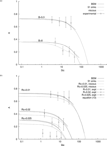
Considering the case when the sampler is pointing vertically downwards. Numerical results have been obtained to compare with the experimental data of Su and Vincent (2003, 2004b) In Figure 6a results are shown for R_C = 0.01 for B = 5.3 and 8. The other values of B considered to compare with the experimental data, namely, B = 10 and 15, were found to give A = 0 for all values of St_C considered. This is due to the fact that for these larger values of B, particles were either collected on the top of the sampler or passed directly by the sampler, none were actually collected through the sampling inlet. This was also found to be the case experimentally by Su and Vincent (2003). As can be seen in the figure all the numerical models predict results which are close to the experimental data. In the case of the potential flow models the results obtained lie within the scatter of the experimental points as shown by their error bars, except for one point. For the viscous flow model all results lie within the experimental error bars. The viscous model does in general, however, predict results which are slightly lower than those predicted by the potential models, especially for B = 8. In Figure 6b results are shown for B = 5.3 for R_C = 0.01, 0.02, and 0.025. As can be seen the potential models predict the experimental results well for R_C = 0.01 but increasingly overpredict the experimental results as R_C increases. This is also the case for the viscous model, where the results for R_C = 0.01 agree very well with the experimental data but for R_C = 0.025 the results are close to the predictions made by the potential models but well above the experimental data. It is unclear why there is such disagreement between the numerical and experimental results for R_C = 0.025. However all three numerical models are in agreement with each other. For this value of R_C conditions are such that the sampling velocities are low and hence air movement minimal making the experiments more difficult. Also, as R_C increases, the measurement of the area enclosed by the limiting particle trajectories is complicated by the fact that the radius of the outer area, r₁, approaches that of the inner area, r₂. More experimental data is necessary to fully understand sampler performance in this parameter range.

Figure 6 Results for the sampler pointing downwards to compare with the experimental data of Su and Vincent (2003, 2004). (a) Aspiration efficiency, A, as a function of Stokes number, St_C, for values of the bluntness parameter B = 8 and 5.3, when the gravitational parameter R_C takes the value 0.01. (b) Aspiration efficiency, A, as a function of Stokes number, St_C, for values of the gravitational parameter R_C = 0.01, 0.02, and 0.025, when the bluntness parameter B takes the value 5.3. BEM denotes results obtained by the Boundary Element Method.

Considering the limiting situation of small St_C when the inertia of the particles can be neglected, it can be shown, see appendix, that no particles will be sampled if B²R_C > 1. If B²R_C < 1, and hence particles are sampled, then as St_C → 0 A → 1 − B²R_C. This explains why A was found to be zero for R_C = 0.01, B = 10 and 15 as discussed earlier. For all cases shown in Figure 6 the numerical results tend towards the predicted value of 1 − B²R_C as St_C → 0.

From Su and Vincent (2003), the reduction in A due to the effect of the blunt sampler body can be expressed as:

Hence the difference in A between a sampler with bluntness parameter B = B₁ and one with bluntness parameter B = B₂ is given by

Therefore the difference between the samplers with values of the bluntness parameter of B = 8 and 5.3 when R_C = 0.01 is approximately 0.36. The numerical results shown in Figure 6a agree with this prediction.

The empirical formula developed by Su and Vincent (2004b) for a blunt sampler pointing downwards is given by:

where k₁ is as given previously in Equation (9). As for the case of pointing upwards this approach is only valid for small values of k₁. Values of this expression are shown in Figure 6b for B = 5.3, R_C = 0.01, 0.02, and 0.025. As can be seen this prediction is also well above the experimental results for R_C = 0.025.

As St_C → 0 in this expression A → 1 − 0.5R_C ^1/2 − R_C (B² − 1) and not 1 − B²R_C as required. Modifying equation (13) to obtain the required limit as St_C → 0 the following expression was obtained.

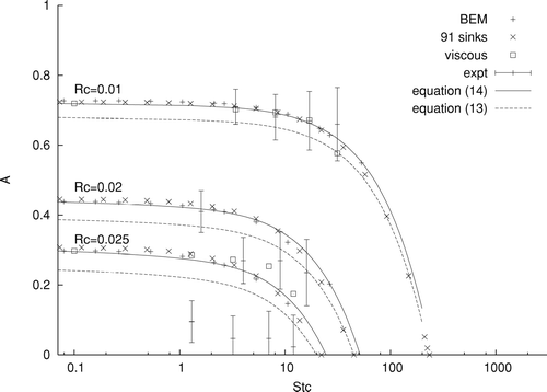
In Figure 7, Equations (13) and (14) are plotted alongside the numerical results, both potential and viscous flow model results, for B = 5.3, R_C = 0.01, 0.02, and 0.025. As can be seen agreement is good between the numerical results and the empirical formula. The agreement does decrease for larger values of St_C but this is expected as the formula is only valid for small k₁ corresponding to small St_C. Similar agreement was found for all results obtained. Agreement is also good between the experimental results and the empirical formula (14) except for R_C = 0.025, where disagreement between experimental and numerical results, and also the earlier empirical formula (13), exists as discussed earlier.

Figure 7 Aspiration efficiency, A, as a function of Stokes number, St_C, for values of the gravitational parameter R_C = 0.01, 0.02, and 0.025 when the bluntness parameter B takes the value 5.3 and the sampler is pointing downwards. Results obtained numerically and experimentally are compared with the 2 empirical expressions (13) and (14). BEM denotes results obtained by the Boundary Element Method.

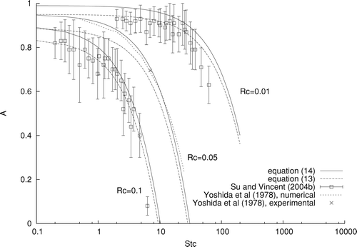
The case of B = 1 corresponds to a thin-walled tube sampler, hence expression (14) has been plotted alongside available numerical and experimental data for this case, in Figure 8. As can be seen agreement is good between the predictions given by Equation (14) and the past work, in particular when comparing with Yoshida et al's (1978) available experimental and numerical data for R_C = 0.05.

Figure 8 Aspiration efficiency, A, as a function of Stokes number, St_C, for values of the gravitational parameter R_C = 0.1, 0.05, and 0.01 when the bluntness parameter B takes the value 1 and the sampler is pointing downwards. Results obtained numerically and experimentally are compared with the 2 empirical expressions (13) and (14).

Numerical calculations were also performed for large values of the parameter B, corresponding to a small sampling orifice relative to the sampler diameter. In these cases it was observed that as well as particle deposition on the sampler head due to gravitational settling, inertial impaction of particles near the suction orifice also occurred. The relative size of the sampling orifice necessary for this effect to be observed was outside the range of values generally taken by real samplers and hence the numerical results have not been shown in this paper.

CONCLUSIONS

From the models developed here, for the case of the sampler oriented with its inlet facing upwards, it is found from the aspiration results and the particle behaviour near the sampler that the bluntness of the sampler has a greater effect upon sampler performance for smaller values of the relative particle settling velocity, R_C. Though for all physically realistic values of R_C the differences in the predicted values of A for different values of B are always small. This is not the case for downwards sampling where the bluntness of the sampler has a bigger effect upon sampler performance. It has been shown here that no aspiration will take place, in this case, if the value of the expression B²R_C is greater than unity. It has also been shown that for small values of the Stokes number, St_C, the aspiration efficiency can be approximated by 1 − B²R_C. A discrepancy was found between the numerical and experimental results for conditions corresponding to low sampling velocities. The numerical results do follow the expected trends and the different numerical models are in agreement. Therefore more experimental data in this region is necessary to understand why this difference occurs and hence better understand sampler performance.

The limiting behavior of A obtained from physical considerations has been used to extend the empirical formulae developed previously for upwards and downwards facing samplers. However these formulae are restricted to a limited range of the parameter involved, a restriction not imposed by the numerical models described here.

Appendix

Limiting case as St_C → 0 for sampler pointing downwards.

Imagine a large sphere, diameter α here α ≫ D, surrounding the sampler. When the sampling rate is Q the number of particles entering this sphere per unit time is

Of these settle on the sampler head, Qc enter the orifice and fall out of the large sphere again, where s is the diameter of the shadow zone below the head.

Hence

c = 0 while s is finite ⇒ π (D² − s²)v_s = 4Q.

Sampling commences when s = 0 ⇒ πD²v_s = 4Q = π δ²U_s

Therefore c > 0, and hence A > 0, for B²R_C < 1, s = 0. In this case

This is for the limiting case of St_C → 0 and hence in the results obtained in this work we would expect that A = 0 for B²R_C > 1 and for situations where B²R_C < 1 as St_C → 0 A → 1 − B²R_C.

REFERENCES

- Agarwal , J. K. and Liu , B. Y. H. 1980 . A Criterion for Accurate Aerosol Sampling in Calm Air . Am. Ind. Hyg. Assoc. J. , 41 : 191 – 197 . [INFOTRIEVE] [CSA]
- Baldwin , P. E. J. and Maynurd , A. O. 1998 . A Survey of Wind Speeds in Indor Workplaces . Ann. Occup. Hyg. , 20 : 303 – 313 . [CSA] [CROSSREF]
- Belyaev , S. P. and Kustov , V. T. 1980 . Sampling from Calm Air . Trudy IEM , 25 : 102 – 108 . (in Russian)[CSA]
- Chung , I. P. and Dunn-Rankin , D. 1993 . The Effects of Bluntness and Orientation on Two-Dimensional Samplers in Calm Air . Aerosol Sci. Technol. , 19 : 371 – 380 . [CSA]
- Davies , C. N. and Peetz , V. 1954 . Dust Shadows Below a Cylinder Containing a Suction Orifice and Deposition of Particles upon the Cylinder . Brit. J. Appl. Phy. , S3 : S17 – 20 . [CSA] [CROSSREF]
- Dunnett , S. J. 2002 . Particle Motion in the Vicinity of a Bulky Sampling Head Operating in Calm Air . Aerosol Sci. Technol. , 36 : 308 – 317 . [CSA] [CROSSREF]
- Dunnett , S. J. and Wen , X. 2002 . A Numerical Study of the Sampling Efficiency of a Tube Sampler Operating in Calm Air Facing Both Vertically Upwards and Downwards . J. Aerosol Sci. , 33 : 1653 – 1665 . [CSA] [CROSSREF]
- Galeev , R. S. and Zaripov , S. K. 2003 . Theoretical Study of Aerosol Sampling by an Idealised Spherical Sampler in Calm Air . J. Aerosol Sci. , 34 : 1135 – 1150 . [CSA] [CROSSREF]
- Grinshpun , S. A. , Lipatov , G. N. and Semonyuk , T. I. 1989 . A Study of Sampling of Aerosol Particles from Calm Air into Thin-Walled Cylindrical Probes . J. Aerosol Sci. , 20 : 1561 – 1564 . [CSA] [CROSSREF]
- Grinshpun , S. A. , Willeke , K. and Kalatoor , S. 1993 . A General Equation for Aerosol Aspiration by Thin-Walled Sampling Probes in Calm and Moving Air . Atmos. Environ. , 27 : 1459 – 1470 . [CSA]
- Kaslow , D. E. and Emrich , R. J. 1973 . Aspirating Flow Pattern and Particle Inertia Effects Near a Blunt Thick-Walled Tube Entrance, Technical Report 23 , PA, USA : Department of Physics, Lehigh Univerisity .
- Kaslow , D. E. and Emrich , R. J. 1974 . Particle Sampling Efficiencies for an Aspirating Blunt Thick-Walled Tube in calm air, Technical report 25 , PA, USA : Department of Physics, Lehigh Univerisity .
- Levin , L. M. 1957 . The Intake of Aerosol Samples . Izvestiya Akademi Naik SSSR Seriya Geofizika. , 7 : 914 – 925 . [CSA]
- Liu , B. Y. H. , Zhang , Z. Q. and Kuehn , T. H. 1989 . A Numerical Study of Inertial Errors in Anisokinetic Sampling . J. Aerosol Sci , 20 : 367 – 380 . [CSA] [CROSSREF]
- Patankar , S. V. 1980 . Numerical Heat Transfer and Fluid Flow, Series in Computational Methods in Mechanics and Thermal Sciences Hemisphere, NY
- Su , W. C. and Vincent , J. H. 2002 . New Experimental Method to Directly Measure Aspiration Efficiencies of Aerosol Samplers in Calm Air . J. Aerosol Sci. , 33 : 103 – 118 . [CSA] [CROSSREF]
- Su , W. C. and Vincent , J. H. 2003 . Experimental Measurements of Aspiration Efficiency for Idealized Spherical Aerosol Samplers in Calm Air . J. Aerosol Sci. , 34 : 1151 – 1165 . [CSA] [CROSSREF]
- Su , W. C. and Vincent , J. H. 2004a . Experimental Measurements and Numerical Calculations of Aspiration Efficiency for Cylindrical Thin-Walled Aerosol Samplers in Perfectly Calm Air . Aerosol Sci. Tech. , 38 : 766 – 781 . [CSA] [CROSSREF]
- Su , W. C. and Vincent , J. H. 2004b . Towards a General Semi-Empirical Model for the Aspiration Efficiencies of Aerosol Samplers in Perfectly Calm Air . J. Aerosol Sci. , 35 : 1119 – 1134 . [CSA] [CROSSREF]
- Vincent , J. H. 1989 . Aerosol Sampling: Science and Practice , Chichester, , UK : John Wiley and Sons .
- Yoshida , H. , Uragami , M. , Hasuda , H. and Iinoya , K. 1978 . Particle Sampling Efficiency in Still Air . Kagaku Kogaku Ronbunshu. , 4 : 123 – 128 . (English translation by the United Kingdom Health and Safety Executive (HSE) translation N 8586)[CSA]