Local and Regional Secondary Organic Aerosol: Insights from a Year of Semi-Continuous Carbon Measurements at Pittsburgh

During the Pittsburgh Air Quality Study (PAQS) an automated semi-continuous thermal-optical transmittance (TOT) carbon analyzer was used to measure 2–4 h average particulate organic (OC) and elemental carbon (EC) concentrations from July 1, 2001 to August 13, 2002. To minimize the adsorption of vapor-phase organics, the sample air was drawn through a multi-channel parallel-plate diffusion denuder placed upstream of the carbon analyzer. Particulate OC and EC in the sample air were then collected on a quartz fiber filter (QFF) mounted inside the carbon analyzer, and analyzed immediately after collection. To account for any remaining organic vapors not retained by the denuder and collected on the sampling filter (positive artifact) a dynamic blank was run every two weeks. An upper-bound estimate of volatilization induced by the presence of the denuder upstream of the sampling filter (negative artifact) was also made. A detailed description of the operating protocol and quality assurance measurements is provided. The contributions of primary and secondary organic aerosol (SOA) to particulate OC were calculated using an “EC tracer method,” which is codified herein. Annual average SOA accounted for 33% of particulate OC. SOA accounted for 30–40% of monthly average OC from June to November in Pittsburgh, similar to previous summertime estimates for Atlanta (Lim and Turpin 2002) and much larger than previous estimates of SOA in the Los Angeles Basin (Turpin and Huntzicke 1995). Examination of concentration dynamics suggests that multi-day formation and regional transport is an important contributor to the higher SOA contributions to OC in Pittsburgh and suggests that SOA is likely to be a particularly important contributor to particulate OC in locations that are recipients of long distance transport, such as the eastern United States.

^†Currently at: Department of Environmental Engineering, Kyungpook National University, Korea.

^††Currently at: Department of Chemical Engineering, Tecnológico de Monterrey, Monterrey, Mexico.

^†††Currently at: Department of Civil and Environmental Engineering, University of Illinois, Urbana-Champaign, IL.

^††††Currently at: Department of Chemical Engineering, University of Patras, Patras, Greece.

INTRODUCTION

Carbonaceous material (total carbon; TC) is a major constituent (10–70%) of atmospheric particulate matter (PM) and a substantial contributor to visibility reduction, climate forcing, and adverse health effects (IPCC 2004; U.S. EPA 2004). Atmospheric carbonaceous PM consists of organic (OC) and elemental carbon (EC) and includes hundreds of organic species with widely varying chemical and physical properties (Turpin et al. 2000)). OC is directly emitted in particulate form (primary) and formed in the atmosphere from semi- and low-volatility products of chemical reactions involving reactive organic gases (secondary; Seinfeld and Pandis 1998; Turpin et al. 2000). EC is produced during incomplete combustion and emitted directly in the particle phase.

Development of effective control strategies for ambient PM requires an understanding of the contributions of primary and secondary OC. Smog chamber experiments have extended our understanding of secondary organic aerosol (SOA) formation mechanisms (Odum et al. 1997; Jang and Kamens 2001). However, there remains a need to estimate primary and secondary OC from field measurements, to test evolving predictive models and to quantify contributions in locations where key model inputs are not available. SOA concentrations have been estimated from measured OC and EC concentrations using EC as a tracer for primary OC (“EC tracer method”; e.g., Turpin and Huntzicker 1995; Strader et al. 1999; Cabada et al. 2004). SOA concentrations have also been predicted using models that couple the formation, transport, and deposition of SOA with atmospheric dynamics (e.g., Strader et al. 1999), and estimated from receptor model results by subtracting the sum of primary source contributions from measured OC concentrations (e.g., Schauer et al. 1996; Schauer and Cass 2000). These three approaches have provided reasonably comparable estimates of SOA in the few locations where comparisons have been made (Turpin and Huntzicker 1995; Strader et al. 1999). However, in most locations outside of southern California the primary and secondary contributions to OC are still largely unknown.

Previous studies have shown that Pittsburgh is a location influenced by SOA production in every period of the year and one where atmospheric conditions and SOA precursor emissions are substantially different from those in southern California (Cabada et al. 2002). This article analyzes in detail semi-continuous OC and EC measurements obtained during the Pittsburgh Air Quality Study (PAQS), provides a codified “EC tracer method,” and uses this method to estimate the primary and secondary contributions to OC at Pittsburgh. Because SOA is best estimated with time-resolved measurements and semi-continuous carbon measurement is only now becoming routine, detailed carbon measurement and quality control protocols are provided and discussed. Concentration dynamics are used to provide insights regarding local and regional sources and atmospheric processing.

EXPERIMENTAL

An automated semi-continuous thermal-optical transmittance (TOT) carbon analyzer (Sunset Laboratory, Beaverton, OR) was used to measure 2–4 h average particulate organic (OC) and elemental (EC) carbon concentrations during the Pittsburgh Air Quality Study (PAQS), from July 1, 2001 to August 13, 2002. This instrument is based on the OGI/Rutgers instrument described elsewhere (Turpin et al. 1990). Instrument performance was previously characterized by Lim et al. (2003a). The field instrument was located inside a climate-controlled trailer on the top of a hill in Schenley Park, near the Carnegie Mellon University campus and about three miles east of downtown Pittsburgh (Wittig et al. 2004). The site was more than 500 m from any major road and was not near any major industrial sources.

During sample collection, ambient air (16.7 L/min) was drawn through a 2.5 μ m aerodynamic diameter cut point cyclone and the flow was isokinetically split between the semi-continuous carbon analyzer (8.7 L/min) and two auxiliary sampling lines, each pulling 4 L/min. During July 2001 each auxiliary sampling line contained a baked 47 mm diameter quartz fiber filter (QFF; QAT-UP, Pall Gelman, Ann Arbor, MI); these were used to conduct volatilization artifact experiments described below. A multi-channel parallel-plate diffusion denuder was placed horizontally upstream of the semi-continuous carbon analyzer to reduce the adsorption of vapor-phase organics on the instrument's sampling filter. The denuder contained 14 strips (8″ × 1.25″) of carbon-impregnated filter (CIF; Schleicher Schuell, Keene, NH) spaced at 2 mm intervals inside an aluminum housing. The semi-continuous carbon analyzer collects particles on a 16 mm diameter QFF punch mounted inside the instrument and analyzes each sample automatically immediately after collection with no sample handling. Eliminating sample handling and storage lowers the instrument detection limits and allows for better time resolution. The carbon analyzer sample collection time was 1.5–3.5 h, yielding collection/analysis cycles of 2–4 h.

Thermal-optical analysis defines OC as the material that volatilizes in the absence of oxygen, whereas EC requires oxygen to combust. Table 1 provides the temperature protocol for semi-continuous carbon analysis during PAQS, and Figure 1 shows a typical thermogram. The protocol was designed to be comparable to the proposed EPA Speciation Trends Network (STN) protocol. The same protocol was used during the Aerosol Characterization Experiment in Asia (ACE-ASIA study; Lim et al. 2003a). In a typical analysis, air is purged and the filter is heated in a helium (He) environment, stepwise, to 870°C to volatilize OC. The main oven temperature is then reduced; the carrier gas is changed to 2% oxygen (O₂) in He, and the temperature is increased stepwise to 880°C to combust EC. In the final step of the analysis, a calibration gas (2% methane in He) is automatically injected for quantitation. All carbon is converted to methane (CH₄) and detected with a flame ionization detector (FID). OC and EC are automatically quantified by dividing their peak areas by the internal calibration peak area and multiplying by the amount of carbon in the calibration peak. After analysis, the QFF is cooled to room temperature and sampling begins again.

FIG. 1 Typical carbon analysis thermogram obtained by the semi-continuous carbon analyzer using the analysis protocol employed during PAQS. Shown are oven temperature (°C), flame ionization detector (FID) signal (shaded area), and laser transmittance. OC, EC, and calibration segments of the FID signal are labeled. The dashed line indicates the introduction of O₂ and the solid vertical line identifies the point at which the laser transmittance regains its pre-pyrolysis value (adjusted for the transit time). Material evolved before this point is considered OC and after, EC.

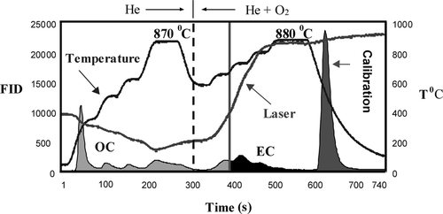
TABLE 1 Temperature protocol used by the semi-continuous carbon analyzer for the analysis of particulate OC and EC during PAQS

Carrier gas	Temperature (°C)	Duration (sec)
He	340	60
He	500	60
He	615	60
He	870	90
He/O2	575	45
He/O2	650	45
He/O2	725	45
He/O2	800	45
He/O2	880	100

While heating a sample in an oxygen-free environment some OC is pyrolitically converted to EC, reducing the transmittance through the filter. Left uncorrected, pyrolysis can lead to substantial bias in OC and EC (but not TC; TC = OC + EC). Therefore a diode laser and photodetector monitor the transmittance of light through the QFF during analysis to correct for the pyrolysis of OC. When oxygen is added, EC evolves increasing the transmittance. The carbon removed to bring the transmittance back to its pre-pyrolysis level is considered to be equal to the pyrolytically-generated EC. Thus, all carbon evolved before this point is reported as OC, and after is EC. The pyrolysis correction assumes either (1) that the original and pyrolytically generated EC have the same absorptivity or (2) that pyrolytically generated EC evolves first. While neither assumption is likely to be completely true, the error introduced is likely to be small relative to the size of the pyrolysis correction.

High purity gases and zero grade air (Matheson Gas Products, Montgomeryville, PA) were used. To remove trace amounts of O₂, the He gas was purified through a series of two O₂ traps (4002, 4004; Alltech, Deerfield, IL) before use. The O₂ trap color indicator showed no color change during the study. All QFFs were pre-baked in a muffle furnace at 550°C for at least 2 h (auxiliary filters) or inside the main oven of the instrument at 870°C for about 4 minutes before collection. The semi-continuous carbon analyzer QFF was replaced every 2–3 days.

QUALITY CONTROL

Quality Control Analyses

Between July 1, 2001 and August 13, 2002 the semi-continuous carbon analyzer was collecting or analyzing samples 80% of the time. (No data were collected September 4–October 11, 2001 due to instrument malfunction and an air traffic moratorium after September 11). Quality control measurements performed during PAQS are summarized in Table 2 and described below.

TABLE 2 Schedule of quality control (QC) activities performed during PAQS

QC activity	Frequency	Duration (min)
Instrument blank	Daily	25
Dynamic blank	Biweekly	35
FID relative response	Biweekly	25
Standard injection	Monthly	25
Filter change	2–3 Days	15
Flow rate check	Monthly	25
Denuder change	4 months	20

An instrument blank was run daily to check for system contamination and any dependence of the laser signal on oven temperature. The instrument blank analytical settings were identical to those used for normal sample analyses, except the instrument was operated with a “zero-second” sampling time. The average instrument blank was 0.1 ± 0.11 (1σ) and 0.01 ± 0.03 μ g C for OC and EC, respectively.

A dynamic blank was run every two weeks to quantify adsorption of any remaining organic vapors (i.e., not retained by the denuder) on the sampling filter (positive artifacts; Turpin et al. 2000)). To collect a dynamic blank, a 47 mm Teflon filter (2 μ m pore, PallGelman, Ann Arbor, MI) was placed upstream of the denuder so that particle-free ambient air was sampled and analyzed (standard analysis protocol) on a 2 or 4 h collection/analysis cycle. Teflon filters employed for the dynamic blank analyses were used as provided by the manufacturer without any pretreatment. The study-average dynamic blank was 0.33 ± 0.11 μ g/m³ (mean ± 1σ), which corresponds to 16% of measured OC. Correction was made for this artifact (see Sampling Artifacts). The denuder material was replaced three times, approximately every four months. No significant change in dynamic blank OC was observed after replacing the denuder material.

To check for variability in the FID response over the course of an analysis a relative response factor analysis was run approximately every 2 weeks. During this analysis a known amount of calibration gas (2% CH₄ in He) is automatically injected upstream of the MnO₂ oven during the He and the He-O₂ analyses segments as well as during the usual calibration segment. The variability of FID sensitivity across an analysis was less than 5% for more than 95% of the study (calibration peak/peak in Helium = 0.97 ± 0.07; calibration peak/peak in He-O₂ = 0.98 ± 0.08). For a small subset of data collected in March 2002, the responses in He and He-O₂ were 90 and 95%, respectively, of the calibration response. These data were corrected for the change in FID response with carrier gas. The quality control measurements above suggest that instrument blank, dynamic blank and relative response factor analyses could have been performed as infrequently as monthly and still meet long term monitoring objectives. However, daily instrument blanks and relative response factor analyses can easily be programmed into the software and performed automatically to provide rapid feedback on instrument performance.

Internal calibration is performed as follows. A certified mixture of CH₄ in He flows continuously through a loop of Teflon tubing inside the analyzer; this loop is switched on line for internal calibration. Therefore, in order to calculate the exact amount of methane injected it is important to know the calibration loop volume. This was measured right before the beginning of PAQS and in advance of the ACE-Asia Study (Lim et al. 2003a) by manually injecting different known volumes of calibration gas (2% CH₄ in He) into the main oven with a 2 ml gas-tight syringe during a standard analysis after “zero-second” collection. The loop volume was calculated by integrating the areas of the resulting peaks and comparing them to the internal calibration peak area. For this instrument the loop volume is 1.63 ml. For a calibration gas containing 2.1% CH₄ in He this corresponds to 17.08 μ g of carbon (μ g C) in the internal calibration peak. Note, efficient conversion of carbon to CO₂ and subsequently to CH₄ is validated on set-up and would have been checked during trouble-shooting if deterioration of peak areas had been observed.

The laser signal responds immediately to the removal of EC from the filter, whereas the FID signal is delayed by the transit time between the sampling filter and the FID detector. Proper alignment of these two signals is essential for the determination of the correct OC-EC split. Changes in an instrument's transit time can occur, for example with replacement of packed columns or changes in plumbing. The transit time was determined prior the beginning of PAQS as the time interval between a rapid increase in optical transmittance with EC evolution and the corresponding increase in the FID signal with arrival of this material (now CH₄) in the FID. The transit time was 5 seconds and did not change perceptibly over the course of the study.

Measurement Uncertainties

A manual injection of calibration gas (2% CH₄ in He, main oven) was performed monthly, and actual and measured carbon mass were always within ± 5% (analytical accuracy). Measurement uncertainty for particulate OC and EC is also impacted by the accuracy of the sampling artifact correction, the accuracy of the pyrolysis correction, and flow rate variability. The flow rates of sample air and analysis gases were checked approximately monthly with a primary flow measurement device (Gilibrator). Measured and actual flow rates were always within 5%. Since each analysis uses the entire sample, determination of the analytical precision by replicate analysis was not possible. However, the analytical precision is expected to be better than that of a laboratory carbon analyzer, which is roughly 4–13% for OC and 6–21% for EC (e.g., Schauer et al. 2003).

During PAQS, the detection limit for OC was 0.43 μ gC (∼ 0.32 μ gC/m³), calculated as three times the standard deviation (3σ) of the dynamic blank OC. Since no dynamic blank EC was ever detected throughout the study, the detection limit for EC was calculated as 3σ of the instrument blank EC, and was 0.15 μ gC (∼ 0.11 μ gC/m³). The OC detection limit for the study is higher than the instrument detection limit, i.e., despite the use of the denuder the detection limit is still dictated by variability in the dynamic blank. The OC detection limit could be reduced further by collecting a dynamic blank concurrently with each sample.

Laser Transmittance

The semi-continuous carbon-analyzer sampling filter is mounted inside the instrument and is typically used for multiple collection-analysis cycles. However, after about 12 hours of operation in Pittsburgh the accumulation of refractory materials such as iron oxide on the filter began to give the filter a red color, decreased the transmittance through the unloaded filter, and caused a temperature-dependent decrease in the transmittance through the filter at the highest temperature steps of the analysis (870 and 880°C). In some samples this temperature-dependent decrease in transmittance caused a delay in the time at which the transmittance regained its pre-pyrolysis value, overestimating the pyrolysis correction and, hence, OC. This phenomenon was also observed during the ACE-Asia study after more than 7 days of continuous operation (Lim et al. 2003a) but not during the Southern California Air Quality Study (SCAQS; Turpin and Huntzicker 1995). During SCAQS deposits of refractory materials were only sufficient to warrant a filter change after approximately one month of continuous operation. To prevent the introduction of errors due to this temperature dependence we normalized the laser signal intensity for each sample analysis (I) by that of the corresponding instrument blank (I_o) and recalculated the OC-EC split for all PAQS measurements (i.e., in accordance with Beer's law). This resulted in an average (± 1σ) correction equivalent to 10 ± 8% of OC when the filter was changed every three days. When analyses were conducted at PAQS with a top OC temperature of 700°C (rather than 870°C), as was done for 40 study days, the temperature dependence was substantially reduced yielding an average OC correction of only 5 ± 7%. Thus, differences in behavior between locations are likely to be due both to differences in the concentration of refractory materials in fine particles and differences in carbon analysis temperature protocols. (The top OC temperature for SCAQS measurements was 700°C.)

A more recent version of the Sunset laboratory calculation program now automatically corrects for the laser temperature dependence (version RT-Calc 114 or newer); PAQS OC and EC data corrected as described above are in excellent agreement with those recalculated using the Sunset laboratory automated correction software (OC: R² = 0.99, Y = 1.01X + 0.02; EC: R² = 0.98, Y = 0.96X − 0.03; where Y is the concentration calculated by RT_Calc114 and X is the concentration calculated manually).

The refractory loading combined with OC analytical temperatures higher than historically used in thermal-optical carbon analysis (i.e., > 700–750°C) also appears to enable some EC to evolve at the highest temperature of the helium analysis segment (870°C), prior to the intentional introduction of oxygen (Chow et al. 2001). The premature evolution of EC could affect the pyrolysis correction and the OC-EC determination, but only if the OC-EC split point were to occur before all OC was able to volatilize or if these conditions somehow affect the accuracy of the pyrolysis assumptions (Subramanian et al. 2006).

Sampling Artifacts

Organic vapors readily adsorb onto QFFs. Unless reduced or corrected for, this positive artifact can cause particulate OC to be substantially overestimated (i.e., 30–40% in urban areas; Turpin et al. 1994, 2000; Mader and Pankow 2001). In this study the adsorption artifact was substantially reduced by placing a denuder upstream of the semi-continuous carbon analyzer. The diffusion of gas-phase material to the denuder carbon strips removes adsorbable vapors but also disturbs the gas-particle equilibrium of semi-volatile species. This could induce volatilization of organic particulate material from the sampling QFF. Therefore, two main issues must be considered: positive artifacts due to denuder breakthrough (estimated by dynamic blank analysis described above) and negative artifacts due to particulate matter volatilization from the sampling QFF. No EC was ever detected in a PAQS dynamic blank analysis (i.e., when sampling particle-free ambient air) ruling out EC contamination from the denuder's carbon strips.

Figure 2 shows the percentage of measured OC that was adsorbed vapor [% of adsorbed vapor = (dynamic blank OC/sample OC) × 100)] for the semi-continuous carbon analyzer measurements made during PAQS, ACE-Asia (Lim et al. 2003a), and the Atlanta supersite study (Lim and Turpin 2002). The use of a denuder upstream of the carbon analyzer during PAQS and ACE-ASIA substantially reduced the adsorption artifact in comparison to the undenuded measurements made in Atlanta. (Note that dynamic blanks were collected concurrently with each sample in Atlanta and subtracted on a sample-by-sample basis to correct for the adsorption artifact.) For both denuded and undenuded systems the adsorption artifact is a larger percentage of measured OC for low OC loadings/concentrations than for high loadings/concentrations. During PAQS, the average adsorption artifact (dynamic blank) was 0.33 ± 0.11 μ g/m³ (1σ) or 16% of the OC measured on the carbon analyzer QFF. It was 33% for the Atlanta study, where an undenuded system was used, even though ambient OC concentrations were higher.

FIG. 2 Percentage of measured OC that is adsorbed vapor (% adsorbed vapor = dynamic blank OC/sample OC) and OC concentrations (μ gC/m³) from the semi-continuous carbon analyzer. Shown are measurements made during the Pittsburgh Air Quality Study (PAQS), Aerosol Characterization Experiment (ACE-Asia), and the Atlanta Supersite study. ACE-Asia and PAQS used a denuder to reduce adsorption.

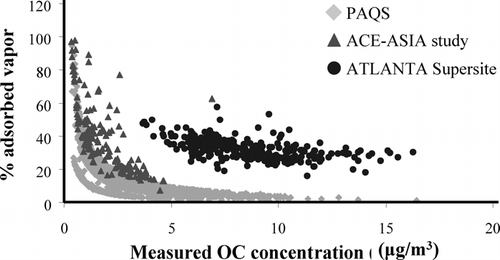
In previous organic artifact experiments conducted without a denuder we have observed an increase in the magnitude of the adsorption artifact with increased loading/concentration of filter-collected OC (e.g., Turpin et al. 1994), even though the percentage of the filter-collected OC that is artifact decreases with increased OC loading/concentration. This makes sense because (1) adsorption is expected to increase with increasing concentrations of organic gases based on equilibrium partitioning and (2) because atmospheric concentrations of organic gases and organic PM are likely to be covariant. However, in this study the magnitude and variability of the adsorption artifact was small and showed no dependence on measured OC. This is presumably because of the use of a denuder that removed adsorbable vapors with high efficiency.

Thus, PAQS OC measurements were corrected for the adsorption artifact to yield particulate OC concentrations as follows. Seasonal average 2 h and 4 h dynamic blank values were subtracted from OC measured on 2 and 4 h sampling/analysis cycles, respectively, to yield particulate OC concentrations. The adsorption estimate for the small number of OC measurements made on a 3 h cycle was estimated by interpolation.

Volatilization of particulate OC from the sampling QFF (negative artifact) could be induced by removal of vapor-phase OC with a denuder. During the first intensive period of PAQS a set of experiments was conducted to provide an upper bound estimate of the magnitude of this type of loss. Six pairs of 24 h integrated samples were collected on QFFs in two auxiliary sampling lines. Six “blow-off” experiments were conducted thereafter by placing a Teflon filter upstream of the denuder inlet, one 47 mm QFF loaded with particulate matter (“loaded” QFF) between the denuder and the semi-continuous carbon analyzer, and operating the instrument in “sampling mode” for 60 to 240 min. The Teflon filter and denuder remove particulate matter and most adsorbable organic vapors present in the sample air, allowing “clean” air to pass through the “loaded” QFF for time periods and at loadings comparable to those used for standard semi-continuous carbon analyzer sample collection. The QFF exposed to “clean” air and the concurrently collected “unexposed” QFF were both analyzed in a laboratory carbon analyzer (Sunset Laboratory, Beaverton, OR). The gaseous OC lost from the “loaded” QFF during these experiments evolved during the first temperature step of the OC-EC analysis (between 25 and 340°C). Volatile losses from the “loaded” QFF were 10 ± 6% (1σ) of the OC loading with no discernable trend with OC loading. Interestingly Subramanian et al. (2004) reported that volatile losses on an integrated denuded PAQS sampler were on the order of 10%. The results from these experiments represent an upper-limit estimate of volatile losses from the semi-continuous carbon analyzer since the loading of particle-phase organics on the carbon analyzer filter normally increases from zero at t = 0, and the amount of OC volatilized from a “loaded” QFF is maximized when the filter is impacted by particle-free air. These findings support the assumption that during PAQS volatilization losses of OC from the semi-continuous carbon analyzer QFF (negative artifacts) were small.

Assessment of Measurement Errors

In summary, the adsorption artifact and the pyrolytic conversion of OC to EC during analysis can introduce substantial errors in the determination of OC and EC by thermal carbon analysis. Optical correction for pyrolysis (thermal-optical carbon analysis) and the use of a denuder reduce these errors substantially. The remaining adsorption artifact at PAQS was 16 ± 13% (0.33 ± 0.11 μ g/m³) and correction for this artifact could easily be made using periodic dynamic blank analyses. Volatile losses appear to be small (< 10 ± 6%) but not well enough quantified to enable correction. Errors introduced into the pyrolysis correction by development of a temperature-dependent laser signal can be large in locations with high concentrations of refractory materials (e.g., Pittsburgh) unless the sample filter is changed every few days. At PAQS this error was reduced from 10 ± 8% (mean ± 1σ) to 5 ± 7% when the top OC analysis temperature was reduced to 700°C. Errors due to flow rate variations and variations in FID response within an analysis can easily be held below 5%. Filter change is the only maintenance activity that requires a technician to visit the site more than monthly.

RESULTS

Organic and Elemental Carbon Concentrations

The study mean OC, EC, and TC concentrations were 2.75 (0.23–15.70), 0.89 (0.20–7.98), and 3.64 (0.43–22.32) μ gC/m³, respectively. Ranges of 2–4 h measurements are given in parentheses. The highest monthly average concentrations were measured in July 2002 (OC = 3.88, EC = 1.13, TC = 5.01 μ gC/m³), while the lowest monthly average concentrations were recorded in January (OC = 1.89, EC = 0.64, TC = 2.53 μ gC/m³) and April 2002 (OC = 1.61, EC = 0.69, TC = 2.30 μ gC/m³). The highest time-resolved OC and TC concentrations measured during PAQS (15.70 and 22.32 μ gC/m³, respectively) were recorded 08 July 2002 (00:00–03:30 EST). The highest EC concentration (7.98 μ gC/m³) was recorded April 17 2002 (04:00–07:30 EST). The concentrations of OC, EC and TC were unexpectedly high in November 2001 and low in April–May 2002.

EC Tracer Method

Using EC as a tracer for primary combustion-generated OC, primary OC (OC_pri) can be described as follows (Turpin and Huntzicker 1995):

where aEC and b are combustion and non-combustion primary OC, respectively. The difference between measured particulate OC (OC_tot) and estimated OC_pri provides an estimate of secondary OC (OC_sec):

An ambient OC to EC ratio that is elevated above the ratio representing the mix of primary combustion sources can result when there is a substantial contribution of secondary OC (SOA) or when EC is very low so that primary non-combustion OC (the intercept, b, in Equation [1]) contributes substantially to the OC to EC ratio.

If a large data set is available and includes times when secondary formation is unlikely, a and b can be determined from a subset of ambient measurements (Turpin and Huntzicker 1995; Strader et al. 1999). The EC tracer method can also be applied to an emission inventory of the principal sources developed for the area of interest (Gray 1986; Cabada et al. 2002). The slope of Equation (1) represents the ratio of primary OC to EC for all contributing combustion sources. It should be noted that primary OC/EC varies with source type. For example the primary OC/EC ratio for biomass burning is much higher than that of diesel PM (Hays et al. 2002). For this reason Equation (1) could vary with location, season, or time of day because of changes in the source mix. Variations in the source mix that have seasonal or diurnal regularity can be identified and accommodated by the EC-tracer method (see below). Occasional irregular contributions from a source with a primary OC to EC ratio vastly different from the usual mix of sources could cause errors in estimated OC_pri and OC_sec during the effected time period(s), but such events are unlikely to affect monthly averages when high frequency measurements are used. If a and b are determined from a data set that is always impacted by SOA, the resulting SOA estimates will be lower bounds.

Estimation of a, b, SOA, and Uncertainties

Time periods when the ambient concentrations of particulate OC were likely to be predominantly primary were identified and used to establish a relationship between primary OC and EC (i.e., to estimate a and b in Equation [1]). For this purpose, hourly concentrations of carbon monoxide (CO) and nitrogen monoxide (NO) were used as indicators of regional and local combustion-related primary emissions, respectively. Hourly ozone (O₃) concentrations and the ratio between nitrogen oxides (NO_x) and NO concentrations were used as indicators of photochemical activity. Time periods were defined as dominated by primary emissions when their 1-h CO and NO concentrations both exceeded the corresponding monthly average and their 1-h O₃ concentration and NO_x/NO concentration ratio were lower than the corresponding monthly averages. Periods with a high probability of SOA formation were defined as times when the 1-h O₃ concentration and NO_x/NO concentration ratio were higher than the corresponding monthly averages. To account for the time necessary for photochemical processes to form SOA, this comparison was made with O₃ and NO_x/NO measurements 0–2 h prior to the time of interest. All other time periods were considered to have a moderate probability of SOA formation. Sampling periods effected by rain were separately identified and were not used in the estimation of a and b because of the possibility of differential wet scavenging (Lim et al. 2003a). (Periods “effected by rain” were identified based on visual observations recorded at the site; “rainy days” means it was raining during sample collection; “after rain” refers to the first sample collected after the rain stopped.)

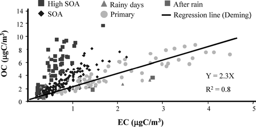
Figure 3 shows particulate OC and EC for all semi-continuous carbon analyzer measurements made during November 2001. Labels segregate data into measurements with a high probability of SOA formation (high SOA), measurements with a moderate probability of SOA formation (SOA), measurements dominated by primary emissions (primary), and measurements impacted by rain events (rainy days; after rain) using the procedure described above. The slope (a) and the intercept (b) in Equation (1) were calculated by regressing OC on EC using only data dominated by primary emissions (circles, Figure 3).

FIG. 3 Particulate OC and EC semi-continuous carbon measurements made during November 2001. High SOA: measurements with a high probability of SOA formation; SOA: measurements with a moderate probability of SOA formation; Primary: measurements dominated by primary emissions; Rainy days and After rain: measurements impacted by rain events. The regression line, equation, and coefficient of determination (R²) were obtained by Deming regression of measurements labeled “Primary.” The intercept was 0 in this case. Similar scatter plots were obtained for each month of PAQS.

To evaluate the impact of different reasonable approaches these regressions were performed on a monthly, seasonal, and annual basis to provide values for a and b in Equation (1). To evaluate whether the primary OC-EC relationship varied because of diurnal variations in the source mix, a and b were also calculated after dividing periods dominated by primary emissions into four different time periods (00:00–06:00; 06:00–12:00; 12:00–18:00; 18:00–00:00 EST). In all cases a Deming linear least-squares regression was used (Deming 1943; Cornbleet and Gochman 1979) and the uncertainties in OC and EC were assumed to be equal. (Conventional linear least-squares regression assumes that there are uncertainties only in the dependent variable.)

Resulting a and b values are provided in Table 3. Month-to-month variations in a and b are not systematic, suggesting that the data could be adequately represented by annually derived values (R² = 0.81). When the data were divided by time-of-day a higher a value (slope) was obtained for the 1200–1800 h time period. This larger value could occur if the mix of primary sources during that time of day typically had a higher primary OC/EC ratio (e.g., due to a reduced contribution from diesel trucks) or if more secondary OC was typically present in the “primary-dominated” data at that time of day. Coefficients of determination (R²) for monthly regressions were all greater than 0.80. Coefficients of determination by season and by time-of-day ranged from 0.74–0.86. Some scatter in primary-dominated data is expected due to variations in the primary source mix. While it is possible that some measurements identified as primary-dominated could have some secondary contribution, selecting the primary ratio based on the lowest OC/EC would ignore the variability in the primary source mix. The fact that the “primary dominated” data resemble a normal distribution around the regression line is reassuring.

TABLE 3 Primary combustion-generated OC/EC (the slope, a, in Equation 1) and primary non-combustion OC (in intercept, b, in Equation 1) calculated by month, season, time-of-day, and annually from a Deming linear least squares regression of OC on EC for data dominated by primary emissions. Shown also are the standard error (SE) of a and b and the coefficient of determination (R²)

Time period	Primary combustion OC/EC (a)	Primary non-combustion OC (b)	R^2	SE (a)	SE (b)
Jul. 2001	2.51	0.00	0.83	0.21	0.36
Aug. 2001	1.64	0.32	0.84	0.13	0.29
Oct. 2001	2.64	0.00	0.82	0.28	0.39
Nov. 2001	2.30	0.00	0.80	0.15	0.34
Dec. 2001	1.89	0.00	0.92	0.07	0.12
Jan. 2002	2.46	0.07	0.85	0.14	0.15
Feb. 2002	2.11	0.18	0.86	0.15	0.23
Mar. 2002	1.81	0.12	0.82	0.13	0.21
Apr. 2002	1.24	0.62	0.88	0.07	0.13
May 2002	1.24	0.66	0.81	0.09	0.15
Jun. 2002	2.38	0.00	0.80	0.20	0.42
Jul. 2002	2.25	0.04	0.85	0.14	0.35
Summer 2001	1.91	0.03	0.79	0.13	0.25
Fall 2001	2.20	0.00	0.86	0.08	0.14
Winter 2002	2.08	0.14	0.81	0.09	0.12
Spring 2002	1.74	0.32	0.74	0.09	0.17
00:00 to 06:00	1.99	0.15	0.76	0.09	0.20
06:00 to 12:00	2.01	0.00	0.85	0.06	0.11
12:00 to 18:00	3.06	0.00	0.75	0.24	0.23
18:00 to 00:00	2.49	0.00	0.82	0.12	0.17
Year	2.07	0.01	0.81	0.04	0.08

Using Equations (1) and (2) and a and b values from each of the 4 approaches in Table 3, primary and secondary OC concentrations were estimated for the duration of PAQS. SOA concentrations estimated from a and b values derived on a monthly, seasonal, annual and time-of-day basis were 0.92 ± 1.11, 1.00 ± 1.16, 1.01 ± 1.14, and 0.85 ± 1.09 μ g/m³ (mean ± 1σ), respectively. The lowest mean SOA concentration was obtained when a and b were calculated separating the data by time-of-day, due to the larger a value obtained for the 1200–1800 h time period. Despite this, the variability in calculated primary and secondary OC concentrations across these four approaches is small, 7% and 11% (pooled coefficient of variation), respectively. This provides confidence in the results and provides one estimate of precision in primary and secondary OC estimates. (This estimate of precision includes “model” uncertainties but does not include measurement uncertainties.) Propagation of error (i.e., including a 10% uncertainty in OC and EC measurements and using the standard error of a and b values) suggests uncertainties in 2–4 h primary and secondary OC estimates are on the order of 10% and 40%, respectively. Below, results using a and b values derived on a monthly basis are reported.

Primary and Secondary OC

The annual average SOA concentration was 0.92 μ g/m³, which represents 33% of the annual average particulate OC. (On a percentage basis 29%, on average, of particulate OC was SOA.) This is in good agreement with the results obtained by Cabada et al. (2002), who developed an emission inventory of primary OC and EC in the Pittsburgh area, applied the EC tracer method to this reconstructed dataset, and concluded that in 1995 the annual SOA contribution to particulate OC was at least 25%. Cabada et al. (2004) independently applied the EC-tracer method to PAQS semi-continuous OC and EC measured from July 1 to August 4, 2001. The same tracers of primary and secondary emissions, but a different decision strategy was used to identify time periods dominated by primary OC. Also Equation (1) was obtained by standard rather than Deming linear least squares regression. For this time period, SOA concentrations of 0.92 ± 0.98 and 1.18 ± 1.05 (mean ± 1σ of time-resolved SOA estimates) were obtained by Cabada et al. (2004) and in the current work, respectively.

During the summer of 2001 and July 2002, SOA was on average 38% of measured OC (SOA = 1.30 μ gC/m³ June–August 2001; 1.44 μ gC/m³ July 2002). This agrees quite well with the contribution of SOA (44%) to particulate OC obtained in Atlanta during August 1999 (Lim and Turpin 2002). The percentage contribution of SOA to particulate OC was much greater for Pittsburgh than for Claremont, CA, where the SOA concentration exceeded 40% of the daily OC concentration only in the afternoon hours of summertime photochemical smog episodes (SCAQS; Turpin and Huntzicker 1995). It should be noted that OC concentrations were much higher in Claremont.

The typical summertime diurnal pattern of carbonaceous species measured/ estimated during PAQS is illustrated in Figure 4. OC and EC peaked between 00:00 and 08:00 EST. Similarly, NO and CO peaked during 00:00–08:00 EST; NO and CO are often used as local and regional combustion tracers. Typically, the summer periods were characterized by high photochemical activity in the afternoon, which resulted in O₃ and SOA concentrations that peaked together between 13:00 and 19:00 EST. This temporal behavior is expected when SOA is formed locally that afternoon. This diurnal pattern was also typical of that observed in the summertime in Atlanta (Supersite; Lim and Turpin 2002). A more pronounced afternoon OC peak was found in Claremont during summertime smog episodes (SCAQS; Turpin and Huntzicker 1995).

FIG. 4 Particulate OC and EC, primary OC (OC_pri), secondary OC (SOA), ozone (O₃), NO, and CO concentrations measured/estimated July 12–19, 2001. This period illustrates typical summertime concentration dynamics.

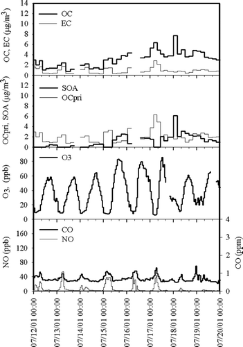
Interestingly, on July 17–19 SOA remained elevated over a 3-day period, even at night. While on previous days the O₃ concentration decreased rapidly at night (perhaps with the aid of NO scavenging), at 00:00 EST, July 18 and July 19 it remained considerably elevated (30 ppb, 45–50% of the peak O₃ concentrations) suggesting either replacement of air from aloft or from upwind. When SOA remains elevated over several days, it is likely that it has been formed through multi-day transport and transformation (i.e., regionally). Regional SOA formation is especially likely aloft where transport distances are great and conditions for photochemistry are favorable. Vertical transport from aloft has been shown to yield elevated nighttime O₃ concentrations (Corsmeier et al. 1997) and would bring SOA formed aloft to ground level as well. Lower nighttime temperatures also contribute to increase the SOA concentration through the favorable partitioning of oxidation products into the particle phase. It was not uncommon for O₃ and SOA concentrations to remain elevated at night. This occurred on approximately 11 nights in the summer and 7 nights in the winter.

A characteristic wintertime period is illustrated in Figure 5. Typically, the concentrations of OC and EC closely tracked those of NO and CO across the day, suggesting that primary combustion sources dominated OC and EC concentrations in the winter. OC and EC concentrations were usually quite low (e.g., February 21–22) but occasionally strong peaks were observed between 02:00 and 08:00 EST, with concentrations substantially higher than those recorded during the summertime, probably because of increased stability and low mixing heights. On February 24, 2002 the OC and EC concentrations peaked between 04:00 and 07:30 EST, reaching values of 8.9 and 4.4 μ gC/m³, respectively, the highest measured winter carbon concentrations.

FIG. 5 Particulate OC and EC, primary OC (OC_pri), secondary OC (SOA), ozone (O₃), NO, and CO concentrations measured/estimated February 21–26, 2002. This period illustrates typical wintertime concentration dynamics.

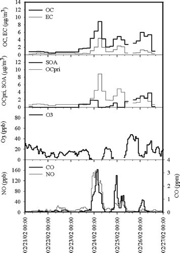
Wintertime SOA and O₃ concentrations measured during PAQS were small compared to the summertime values, but there were times when the EC-tracer method suggested SOA formation. For example, between February 24 and February 26, 2002 peak concentrations of NO, CO, and EC decreased. OC decreased initially and then increased during this period. While the O₃ concentration is still reasonably low, it reached a maximum for this February time period (36 ppb) on February 25, just as the calculated SOA concentration began to increase. It is likely that the elevated ozone peak on February 25 occurs as a result of down-mixing of air from aloft rather than local photochemical formation. This air mass had an elevated OC/EC ratio, suggesting either regional secondary formation or regional transport of a primary carbon source with a high OC/EC ratio (e.g., biomass burning). OC/EC ratios from open burning of biomass can be quite high; transport to Pittsburgh from the southeastern US commonly occurs, and prescribed burning is practiced in the Southeast in the fall/winter (Hays et al. 2002). Thus, the later possibility cannot be ruled out, and illustrates a potential limitation in the EC-tracer method in locations where regional transport is substantial. It should be noted that the decrease in peak CO on February 26 does not support a primary regional combustion origin for the additional OC. The quantity of SOA formed regionally over several days is likely to depend in a complicated way on the integrated exposure of precursors to oxidants (e.g., ozone and hydroxyl radical) during transport (e.g., from the southeastern U.S.). Regional formation could occur as a result of gas-phase, surface, or aqueous-phase reactions in clouds or aerosols (Odum et al. 1997; Jang and Kamens 2001; Lim et al. 2005). On February 26 the calculated primary and secondary OC concentrations were roughly equal. SOA formation was reported to account for 20% of wintertime OC on average with short peaks as great as 60% in the San Joaquin Valley, CA (1995–96; Strader et al. 1999). The average wintertime (2002, Pittsburgh) SOA concentration calculated herein was 24% of measured OC (0.56 μ gC/m³).

Fall 2001 and spring 2002 were characterized by an average SOA concentration of 0.92 and 0.61 μ gC/m³, corresponding to 28 and 20% of OC, respectively. Daily OC and EC concentration dynamics in the fall were more similar to those observed in the summer, but OC, EC, and SOA maxima were generally smaller. Spring concentration dynamics were more similar to those observed in the winter. March–May had many precipitation events (a total of 144 h with greater than 25 mm of rain), which contributed to the low springtime PM concentrations. The lowest monthly mean SOA concentration (0.27 μ gC/m³; 14% of OC) occurred in April, probably as a result of both low photochemical activity and considerable precipitation.

November 2001 had three time periods when EC dropped or remained low while OC increased dramatically. These are shown in Figure 6 as Episodes A, B, and C. Episode A occurred on 01–03 November. During that period O₃ and OC increased and remained elevated for almost 48 h with no increase in the primary combustion tracer, EC. Then, at the onset of precipitation, OC and O₃ decreased rapidly. Episode B occurred on November 14–18, to following 2–3 days of very high concentrations of the primary tracers (EC, CO, and NO), as well as high OC concentrations. Rapid decreases in EC, CO, and NO were followed by a 2–3 day period of continuously elevated O₃ accompanied by a peak and a gradual decrease in OC. Episode C occurred on November 19 and was characterized by increasing OC and O₃ and decreasing EC, CO, and NO.

FIG. 6 (a) Particulate OC and EC, primary OC (OC_pri), secondary OC (SOA), ozone (O₃), NO and CO concentrations measured/estimated October 31–November 30, 2001. High average SOA in November was mostly due to three SOA formation episodes: A (November 1–3), B (November 14–18), and C (November 19). (b) Secondary organic aerosol (SOA; μ gC/m³) and sulfate (μ g/m³), October 31–November 17, 2001. Episode A: November 1–3; Episode B: November 14–18.

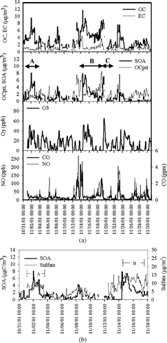
The ozone concentrations during these episodes were not high by summertime standards and might not provide sufficient oxidant concentrations to form SOA locally. Ground level ozone concentrations are often quite low due to titration by primary pollutants, such as NO. The elevated ozone concentrations likely occur because ozone is being mixed down to the surface from aloft (or perhaps transported in from an upwind location). What is apparent in Episodes A and B is that when ozone is replenished it brings an air mass elevated in OC but not in EC. Pollutants can be transported long distances aloft under conditions that are conducive to photochemistry. Thus it is quite plausible that this additional OC is SOA. During Episode A, the EC tracer method calculated SOA concentrations that remained between 4.0 and 8.0 μ gC/m³ (60–85% of OC) over a 24-h period. During Episode B, the calculated SOA maximum was 7.5 μ gC/m³ (79% of OC) and occurred at 00:00–02:00 EST on November 15. During both Episodes A and B, sulfate (a secondary species formed regionally through gas and aqueous phase reactions) also remained elevated (see Figure 6b). SOA and O₃ concentrations that increased and remained elevated over a few days were observed many times during PAQS, during the winter and summer.

It is possible that such concentration dynamics could occur due to the influence of a large primary source with a high OC/EC ratio and no temporal regularity (e.g., wildfires or prescribed burning) located distant from Pittsburgh (e.g., the southeastern U.S.). Down-mixing of these pollutants from aloft could cause a sudden increase in OC without a concurrent increase in EC. OC/EC ratios from biomass burning can be greater than 10 (Hays et al. 2002). The possibility that calculated SOA is really primary OC from biomass combustion cannot be entirely ruled out for these two November episodes. However, the similar SOA and sulfate dynamics supports secondary formation. Additionally, the regional combustion tracer, CO, was highly correlated with primary OC (R² = 0.82) and uncorrelated with calculated SOA.

The largest limitation of the analysis above occurs because of the potential for confounding by biomass burning. While we did not identify any local or more distant prescribed burns that would bias the assessment of SOA, it would be quite difficult to rule out such confounding based on emissions information, which is rarely complete. However, tracer compounds can provide useful insights. Molecular source tracers, including biomass smoke tracers (i.e., levoglucosan, syringols, and resin acids) were measured at PAQS daily in July and every 6th day the remainder of the year. An upper limit of 2%, 14.5%, and 10% of OC was attributed to biomass burning during the summer, fall and winter, respectively, when molecular source tracers were used in chemical mass balance source apportionment (Robinson et al. 2006). Biomass smoke tracer concentrations were quite low during July. Using the average levoglucosan concentration (10 ng/m³) during the July 12–20 time period (Figure 4) and the levoglucosan to OC ratio (0.094) of Lee et al. (2005), biomass smoke contributed only 0.1 μ gC/m³, with a peak of 0.17 μ gC/m³ on 17 July. The highest biomass smoke marker concentrations were measured in October and November, with levoglucosan reaching 73 and 192 ng/m³ on November 2 and 14, respectively. This corresponds to roughly 0.7 and 2.0 μ gC/m³ of biomass OC (SOA ranged from 4–8 μ gC/m³ on these days). Thus, biomass burning could contribute to, but does not appear to explain completely, the elevated OC concentrations observed in November. Biomass markers were not measured during the February 24–26 period, although the PAQS molecular marker data show surprisingly little influence of biomass smoke in the winter (Robinson et al. 2006).

CONCLUSIONS

During the Pittsburgh summertime, SOA was a much more substantial contributor to particulate OC than in the Los Angeles Basin (Claremont, CA; 1987 SCAQS; Turpin and Huntzicker 1995), although Claremont concentrations were greater. In Claremont, SOA only exceeded 40% of OC during the afternoon hours of summertime photochemical smog episodes. In contrast, the summertime average SOA contribution was nearly that great in Pittsburgh (38% of particulate OC). Summer periods in Pittsburgh were often characterized by early morning peaks in OC and EC and late afternoon peaks in O₃ and SOA. This pattern is consistent with local formation of SOA. However, the EC tracer method produced the highest SOA concentration estimates at times when O₃ and OC increased and remained elevated over several days. This ozone pattern suggests down-mixing of ozone and other species from aloft, where pollutants can be transported long distances and are exposed to conditions conducive to photochemistry. The elevated OC relative to EC combined with low CO and complementary sulfate dynamics during these episodes is consistent with multi-day regional SOA formation, although regional transport of primary OC from biomass combustion cannot be completely ruled out.

These findings suggest that SOA could be an important contributor to particulate OC in locations that are recipients of long distance transport (e.g., the eastern United States) and regional sulfate formation. Neither in-cloud formation (Ervens et al. 2004; Lim et al. 2005) nor acid-catalyzed surface reactions (Jang and Kamens 2001) are currently included in predictive models and are likely to contribute to regional SOA formation.

We gratefully acknowledge the hospitality and assistance of our Carnegie Mellon University hosts. We appreciated the encouragement of PAQS' neighbor, Mr. Fred Rogers, and wish to thank David Smith and Bob Cary at Sunset Labs for their continued assistance. This work was supported in part by the US Department of Energy, US Environmental Protection Agency, and the NJ Agricultural Experiment Station. This research has not been subjected to Agency review and therefore does not necessarily reflect the views of DOE or EPA; no official endorsement should be inferred.

Notes

^†Currently at: Department of Environmental Engineering, Kyungpook National University, Korea.

^††Currently at: Department of Chemical Engineering, Tecnológico de Monterrey, Monterrey, Mexico.

^†††Currently at: Department of Civil and Environmental Engineering, University of Illinois, Urbana-Champaign, IL.

^††††Currently at: Department of Chemical Engineering, University of Patras, Patras, Greece.

REFERENCES

- Cabada , J. C. , Pandis , S. N. and Robinson , A. L. 2002 . Sources of atmospheric carbonaceous particulate matter in Pittsburgh, Pennsylvania . J. Air Waste Manag. Assoc. , 52 : 732 – 741 . [INFOTRIEVE] [CSA]
- Cabada , J. C. , Pandis , S. N. , Subramanian , R. , Robinson , A. L. , Polidori , A. and Turpin , B. J. 2004 . Estimating the secondary organic aerosol contribution to PM2.5 using the EC tracer method . Aerosol Sci. Technol. , 38 : 140 – 155 . [CROSSREF] [CSA]
- Chow , J. C. , Watson , J. G. , Crow , D. , Lowenthal , D. H. and Merrifield , T. 2001 . Comparison of IMPROVE and NIOSH carbon measurements . Aerosol Sci. Technol. , 34 : 23 – 34 . [CSA]
- Cornbleet , P. J. and Gochman , N. 1979 . Incorrect least-squares regression coefficients in method-comparison analysis . Clin. Chem. , 25 : 432 – 438 . [INFOTRIEVE] [CSA]
- Corsmeier , U. , Kalthoff , N. , Kolle , O. , Kotzian , M. and Fiedler , F. 1997 . Ozone concentration jump in the stable nocturnal boundary layer during a LLJ-event . Atmos. Environ. , 31 : 1977 – 1989 . [CROSSREF] [CSA]
- Deming , W. E. 1943 . Statistical Adjustment of Data , New York, NY : Wiley .
- Ervens , B. , Feingold , G. , Frost , G. J. and Kreidenweis , S. M. 2004 . A modeling study of aqueous production of dicarboxylic acids: 1. Chemical pathways and speciated organic mass production . J. Geophys. Res. , 109 doi:10.1029/2003JD004387[CSA]
- Gray , H. A. 1986 . Control of atmospheric fine primary carbon particle concentrations , EQL Report No. 23 103 – 108 . Pasadena, California : Environmental Quality Laboratory, California Institute of Technology .
- Hays , M. D. , Geron , C. D. , Linna , K. J. , Smith , N. D. and Schauer , J. J. 2002 . Speciation of Gas-Phase and Fine Particle Emissions from Burning of Foliar Fuels . Environ. Sci. Technol. , 36 : 2281 – 2295 . [INFOTRIEVE] [CROSSREF] [CSA]
- Intergovernmental Panel on Climate Change (IPCC) . 2001 . Climate Change 2001: The Scientific Basis , 944 UK : Cambridge University Press .
- Jang , M. S. and Kamens , R. M. 2001 . Atmospheric secondary aerosol formation by heterogeneous reactions of aldehydes in the presence of a sulfuric acid aerosol catalyst . Environ. Sci. Technol. , 24 : 4758 – 4766 . [CROSSREF] [CSA]
- Lee , S. , Baumann , K. , Schauer , J. J. , Sheesley , R. J. , Naeher , L. P. , Meinardi , S. , Blake , D. R. , Edgerton , E. S. , Russell , A. G. and Clements , M. 2005 . Gaseous and particulate emissions from prescribed burning in Georgia . Environ. Sci. Technol. , 39 : 9049 – 9056 . [INFOTRIEVE] [CROSSREF] [CSA]
- Lim , H. J. , Carlton , A. G. and Turpin , B. J. 2005 . Isoprene forms secondary organic aerosols through cloud processing: Model simulations . Environ. Sci. Technol. , 39 : 4441 – 4446 . [INFOTRIEVE] [CROSSREF] [CSA]
- Lim , H. J. and Turpin , B. J. 2002 . Origins of primary and secondary organic aerosol in Atlanta: Results of time-resolved measurements during the Atlanta supersite experiment . Environ. Sci. Technol. , 36 : 4489 – 4496 . [INFOTRIEVE] [CROSSREF] [CSA]
- Lim , H. J. , Turpin , B. J. , Russell , L. M. and Bates , T. S. 2003a . Organic and elemental carbon measurements during ACE-Asia suggest a longer atmospheric lifetime for elemental carbon . Environ. Sci. Technol. , 14 : 3055 – 3061 . [CROSSREF] [CSA]
- Lim , H. J. , Turpin , B. J. , Edgerton , E. , Hering , S. V. , Allen , G. , Maring , H. and Solomon , P. 2003b . Semicontinuous aerosol carbon measurements: Comparison of Atlanta Supersite measurements . J. Geophys. Res. , 108 ( D7 ) Art. No. 8419[CROSSREF] [CSA]
- Mader , B. T. and Pankow , J. F. 2001 . Gas/solid partitioning of semivolatile organic compounds (SOCs) to air filters. 3. An analysis of gas adsorption artifacts in measurements of atmospheric SOCs and organic carbon (OC) when using Teflon membrane filters and quartz fiber filters . Environ. Sci. Technol. , 35 : 3422 – 3432 . [INFOTRIEVE] [CROSSREF] [CSA]
- Odum , J. R. , Jungkamp , T. P. W. , Griffin , R. J. , Flagan , R. C. and Seinfeld , J. H. 1997 . The atmospheric aerosol-forming potential of whole gasoline vapor . Science , 276 : 96 – 99 . [INFOTRIEVE] [CROSSREF] [CSA]
- Robinson , A. L. , Subramanian , R. , Donahue , N. M. , Bernardo-Bricker , A. and Rogge , W. F. 2006 . Source apportionment of molecular markers and organic aerosol—2. Biomass smoke . Environ. Sci. Technol. , submitted[CSA]
- Schauer , J. J. , Rogge , W. F. , Hildemann , L. M. , Mazurek , M. A. and Cass , G. R. 1996 . Source apportionment of airborne particulate matter using organic compounds as tracers . Atmos. Environ. , 30 : 3837 – 3855 . [CROSSREF] [CSA]
- Schauer , J. J. and Cass , G. R. 2000 . Source apportionment of wintertime gas-phase and particle-phase air pollutants using organic compounds as tracers . Environ. Sci. Technol. , 34 : 1821 – 1832 . [CROSSREF] [CSA]
- Schauer , J. J. , Mader , B. T. , Deminter , J. T. , Heidemann , G. , Bae , M. S. , Seinfeld , J. H. , Flagan , R. C. , Cary , R. A. , Smith , D. , Huebert , B. J. , Bertram , T. , Howell , S. , Quinn , P. , Bates , T. , Turpin , B. , Lim , H. J. , Yu , J. and Yang , C. H. 2003 . ACE-Asia intercomparison of a thermal-optical method for the determination of particle-phase organic and elemental carbon . J. Geophys. Res. , 37 : 993 – 1001 . [CSA]
- Seinfeld , J. H. and Pandis , S. N. 1998 . Atmospheric Chemistry and Physics: From Air Pollution to Global Change , New York : John Wiley and Sons Inc. .
- Strader , R. L. , Lurmann , F. and Pandis , S. N. 1999 . Evaluation of secondary organic aerosol formation in winter . Atmos. Environ. , 33 : 4849 – 4863 . [CROSSREF] [CSA]
- Subramanian , R. , Khlystov , A. Y. , Cabada , J. C. and Robinson , A. L. 2004 . Positive and negative artifacts in particulate organic carbon measurements with denuded and undenuded sampler configurations . Aerosol Sci. Technol. , 38 : 27 – 48 . [CROSSREF] [CSA]
- Subramanian , R. , Khlystov , A. Y. and Robinson , A. L. 2006 . Effect of peak inert-mode temperature on elemental carbon using thermal-optical transmittance . Aerosol Sci. Technol. , in press[CSA]
- Turner , J. R. and Hering , S. V. 1994 . The additivity and stability of carbon signatures obtained by evolved gas analysis . Aerosol Sci. Technol. , 21 : 294 – 305 . [CSA]
- Turpin , B. J. , Cary , R. A. and Huntzicker , J. J. 1990 . An in situ, time-resolved analyzer for aerosol organic and elemental carbon . Aerosol Sci. Technol. , 12 : 161 – 171 . [CSA]
- Turpin , B. J. , Huntzicker , J. J. and Hering , S. V. 1994 . Investigation of organic aerosol sampling artifacts in the Los Angeles basin . Atmos. Environ. , 28 : 3061 – 3071 . [CROSSREF] [CSA]
- Turpin , B. J. and Huntzicker , J. J. 1995 . Identification of secondary organic aerosol episodes and quantification of primary and secondary organic aerosol concentration during SCAQS . Atmos. Environ. , 29 : 3527 – 3544 . [CROSSREF] [CSA]
- Turpin , B. J. , Saxena , P. and Andrews , E. 2000 . Measuring and simulating particulate organics in the atmosphere: problems and prospects . Atmos. Environ. , 34 : 2983 – 3013 . [CROSSREF] [CSA]
- U.S. Environmental Protection Agency [U.S. EPA] . 2004 . Air Quality Criteria for Particulate Matter , Vols. 1 and 2 , Research Triangle Park, NC : Office of Research and Development .
- Wittig , A. E. , Anderson , N. , Khlystov , A. Y. , Pandis , S. N. , Davidson , C. and Robinson , A. L. 2004 . Pittsburgh air quality study overview . Atmos. Environ. , 38 : 3107 – 3125 . [CROSSREF] [CSA]