Unipolar Field and Diffusion Charging in the Transition Regime—Part II: Charging Experiments

Abstract

Unipolar charging of narrowly distributed 30–100 nm DEHS aerosols in air is investigated, in order to determine the influence of the external electric field (E ₀ ≤ 5 kV/cm) and high charging intensities (n·t ≤ 5 · 10 ¹⁴ s/m ³ ) on the charging efficiency. The results are compared with a combined diffusion and field charging model based on the limiting-sphere concept described in Part I.

The experiments were carried out in a wire corona charger under conditions of complete radial turbulent mixing, which makes the determination of charging history straightforward and very accurate. The state of mixing was verified on the basis of the Deutsch model, by separate measurements of particle losses.

For positive charging, the agreement between measured and predicted mean charge was generally better than 5% for particles larger than 45 nm, which typically carried more than 4 unit charges; for 30 nm particles and relatively low charge levels the uncertainties in the model lead to deviations up to 30%.

In case of negative charging, the observed charge levels progressively exceeded those predicted on the basis of mean ion mobilities by factors up to 2 as the charging intensity increased, and there was evidence of additional charging by free electrons.

1. INTRODUCTION

Efficient unipolar charging of aerosols under 100 nm is important for many practical reasons ranging from improved measurement techniques to more efficient electrostatic precipitation. It was shown theoretically in Part I that the application of an additional external electric field is indeed a promising way to enhance ion diffusion charging in the transition regime, thereby allowing higher charge levels and reduced charging times.

While there are numerous theoretical studies dedicated to diffusion charging in the transition regime which are well validated by measurements (e.g., Kirsch and Zagnit'ko 1981; Adachi et al. 1985; Pui et al. 1988; Romay and Pui 1992; Biskos et al. 2005), the combination of field and diffusion charging in the transition regime has hardly been investigated at all. Due to this lack of theoretical and experimental investigations, the literature has remained controversial regarding the benefit of an external field in the transition regime (see Part I). For example the experiments of Kirsch and Zagnit'ko (1981) with sub-100 nm particles do not show an effect of electric fields up to 6.5 kV/cm. Later field charging studies have dealt only with particles larger than 100 nm (e.g., Kirsch and Zagnit'ko 1990)—a size range which ceases to belong to the transition regime under conditions of STP. A very good compilation of these (mostly) continuum field charging experiments is given by Lawless (1996).

As discussed in Part I, the theoretical difficulties lie in the treatment of the complete electrostatic potential function, which destroys the spherical symmetry of the problem. A new 2-D limiting-sphere model was presented there, which indeed predicts a significant influence of the external field on the charging process. This second paper provides the necessary experimental validation of these predictions.

An electrical field in the charging zone invariably leads to significant particle transport and fluid mixing, and thereby to particle losses as well as to the movement of particles between regions of different field and ion densities. Any experimental study therefore has to create the appropriate environment where the data can be interpreted unambiguously with regard to particle charging history (needed for a comparison with theory) and particle losses (which must not alter the mean exit charge relative to the intrinsic charge level). The conventional wisdom is to minimize losses by establishing laminar flow in the charging zone; this also ensures that the particles follow streamlines of defined n· t product. In a recent study however, Marquard, Meyer, and Kasper (2006a, 2006b) have pointed out that this approach is not necessarily the best for very small particles. The high ion densities required for efficient charging tend to produce a strong ion wind which disrupts the laminar flow and tends to increase particle losses, which are already significant due to the high particle mobilities combined with longer residence times. For nanoaerosols this problem arises for pure diffusion charging, and a strong external electric field will increase the losses even further. The concept of providing undisturbed laminar flow conditions, low E₀-values and homogenous ion distributions within the charger (for pure diffusion charging experiments) thus needs to be revisited for field charging experiments with nanoaerosols.

In Section 2 we present a suitable experimental strategy for providing well-defined charging conditions in electric fields (here up to 5 kV/cm) and ion concentrations (here up to 5 · 10¹⁵ m^{− 3})—a regime which is both technically relevant and easily attainable. Particular attention is given to determination of the charging conditions (Section 3), and in Section 4 to the verification of the mixing state of the particles, which is crucial for a well-defined charging history. The data on particle charge and loss data are compared with model predictions in Sections 5 and 6.

2. EXPERIMENTAL STRATEGY, SET-UP, AND PROCEDURES

The overall experimental strategy is based on the fact that it is impossible to create an experimental environment, which combines low particle losses with strong electric fields and high ion concentrations on one hand and well-defined charging conditions on the other hand (the latter are essential for charging model validation). The idea therefore is to accept particle losses and non-uniform electric conditions within the charger, but to make sure nonetheless that the sampled particles have representative average charging histories. One way to do this is to ensure that the particles within the charger are radially well mixed, for example by turbulent flow. Under conditions of ideal mixing one can accept a charger with a radial ion concentration profile without requiring complicated analyses to determine the n· t-product. The n· t-product can simply be calculated from independent averages of residence time t and ion concentration n_i. This strategy further makes use of the fact that the ion space charge flattens out the radial E-Field so that one can work with a quasi-constant field E₀ in the charging zone (compare Part I).

A note of caution is required nevertheless regarding the above strategy: Generally, in case of spatially distributed charging conditions a more complex treatment would be required (see, e.g., Marquard et al. 2006b). This means here, if the E-field in the charging zone has a pronounced profile (in the simplest case as one-dimensional radial profile E₀(r)), and if this external E-field has a non-linear effect on the charging process, then working with average values of E₀ would be inadmissible.

We will show later on, that the charger design chosen here—a wire-tube electrostatic precipitator (ESP) depicted in Figure 1—fulfills the requirements devised above. It consists of a cylindrical tube (L = 26 cm, Ø_tube = 4 cm, or 2.5 cm) with a coaxial tungsten wire (Ø_wire = 0.1 mm). In this “direct corona” arrangement ions are generated and mixed with particles within the same chamber. The length of the corona discharge region was adjusted to L_c = 24 cm or 5 cm by shielding the ends of the wire, while at the same time eliminating undefined end effects in the charging zone of the chamber. The average carrier gas flow velocity was varied between 0.55 m/s and 3.9 m/s, covering tube Reynolds numbers from 1500 to 7000.

FIG. 1 Corona charger (wire-tube ESP design). Flow direction and sampling positions 1 to 6 as indicated, with Pos. 3 to 6 optional. Active corona length L_c limited by shielding tubes of different lengths at both ends (bold: L_c = 24 cm; open: L_c = 5 cm). Light gray areas: insulating material (PVC); dark gray: metal.

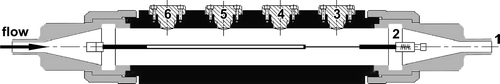
The charger shown in Figure 1 had various sampling ports numbered 1 to 6. For charge measurements, sampling was mostly done from Port 2 (outlet cone removed), because Port 1 was found to produce additional losses caused by the local field between wire mount and insulator wall surface (see also Section 4 for an analysis of particle losses). The ports numbered 3 to 6 were optional in order to vary the residence time as required.

The experimental set-up for generating and characterizing the aerosol uses rather conventional techniques. The monodisperse aerosol generation part consists of an evaporation/condensation process followed by classification and neutralizing steps employing radioactive sources, DMA and a “passive” ESP (air gap plate capacitor). So, the resulting test aerosol comprised of uncharged DEHS droplets (ϵ_P = 4) with narrow size distribution (σ_g ≤ 1.15) dispersed in dry, filtered air. Low particle concentrations (c = 10⁴ cm^{− 3}) and particle sizes between 30 and 100 nm were chosen to meet the assumptions of the charging model to be validated as closely as possible, i.e., negligible particle space charge and spherical particles in a size range where diffusion losses are negligible; the smallest particle diameter covers the lower size limit for the Fuchs theory; charging of isolated particles (for more details see Marquard et al. 2006b).

The techniques and procedures for measuring the mean particle charge can also be considered standard: Particle losses were determined by simultaneously measuring particle number concentrations at inlet and outlet of the charger (by means of a condensation particle counter CPC 3010, TSI Inc); average charges were measured by means of an aerosol faraday cup electrometer (FCE, own design) in addition to the concentration measurements; particle size distributions were checked by a scanning mobility particle sizer (SMPS 3934, TSI Inc.). The measured variables include the exit average charge q _exit and the total particle loss as defined by Marquard et al. (2006a).

In order to minimize experimental errors, all measurements were calibrated carefully. Particle size measurements were carried out with different SMPS systems (DMA operation with 1 l/min sample flow and 10 l/min sheath air flow). The error with regard to particle size was quantified to be less than 3%. For the charge calibration measurement samples were taken from the outlet of the classifier. Here, particles are expected to carry one elementary charge. Since the monodisperse aerosol always was selected at the peak of the adjusted polydisperse raw aerosol size distribution (lognormal distributed, σ _g ≈ 1.5), or closely at the right hand side of the peak, the existence of multiply charged particles could be neglected (additional size distribution measurements of the monodisperse [more precisely: monomobile] aerosol showed the fraction of particles with higher electric mobility always being less than 5%). The error of q _exit values was found from the calibration experiments to be less than ± 5%. This value results from observed deviations of average charge values at the DMA outlet, which were measured before and after measurement series (with two minute averaging time for a single charge value).

3. DETERMINATION OF CHARGING CONDITIONS

In order to model particle charging in the corona charger as described in Part I, one needs to know the radial profiles of ion concentration and electric field, n_i(r) and E₀(r), as well as the residence time t of the particles in the charging zone.

Based on the assumption of plug flow in the charger region (which will be substantiated in the following section), the residence time t is simply the ratio of charger volume V and volumetric flow rate Q.

In order to determine the radial profiles of ion concentration and electric field, a few remarks on corona modeling are required. Corona systems are modeled along two different routes. The more general approach is based on the concept of effective ionization coefficients by Townsend (1915) (see, e.g., Gallimberti, 1979, 1998) and covers arbitrary electrode geometries. Simpler approaches for wire-plane (e.g., Sigmond 1986; Jones 1992) or wire-tube coronas (e.g., Jones et al. 1988) use the Kaptzov-condition (Kaptzov 1947) and apply the Peek-formula (Peek 1929; Hartmann 1984). Mostly a discrete radius for the corona zone is assumed, which divides regions with bipolar and unipolar charge carriers.

We chose a simplified approach of the latter route, which is also quite common: Since the active corona zone is usually very small (here, according to Jones et al. 1988, it is estimated to fill out less than 0.1% of the total charger cross section), it was neglected, effectively treating the entire geometrical cross section starting from the wire surface as unipolar with appropriately chosen boundary conditions obtained by simultaneous measurements of corona voltage and current. (For a closer analysis regarding the treatment of the active corona zone see Jones et al. 1988.)

Within the unipolar zone the profiles for E₀ and n_i are solutions of the electrostatic equations (Poisson equation, Equation [1], and equation of current continuity Equation [3]), which lead to a PDE system for the electrostatic potential and the ion concentration n_i (= space charge density ρ _i /elementary charge unit e). For negligible particle space charge ρ _P , (which is admissible in this paper) in Equation (1) and Equation (4) the total space charge ρ = ρ_i+ ρ_P can be set to ρ _i . Since we have neglected the corona region, we can choose Dirichlet conditions for ϕ on all boundaries and a fixed ion flux j _i (Equation [3]) from the corona electrode. Mathematically the problem is well posed (uniqueness shown by Sheng et al. 1988).

Inserting the Nernst-Townsend-Smoluchowski-Einstein relation

into Equation (3) and Equation (4), assuming Z_i to be constant and neglecting the convective contribution to ion transport gives the simplified continuity equation for the mobility specific ion flux j:

The common assumption of constant Z_i (i.e., constant ion mass) is of course a very rough simplification for a direct corona, given that ion clustering and aging probably take place in the charger during the entire ion lifetime of a few hundreds of microseconds (e.g., Mohnen, 1974). Unfortunately, cold plasma processes (e.g., Capitelli 2000; Hippler 2001; Brown 2004) and their relationship to the impurities in the carrier gas are not understood well enough to provide valid ion aging data for practical aerosol applications, even when using bottled air. Using constants for Z_i is therefore still the most reasonable way to evaluate the electric conditions within a corona charger. (Z_i-profiles would add terms to Equation [4] and Equation [6], and thus alter the electric charging conditions significantly, e.g., Marquard 2006.) The concept of using average ion data finally brakes down in the presence of free electrons (e.g., Romay and Pui 1992a; Wiedensohler and Fissan 1988).

As described above, the charger design and operating parameters were chosen to permit the use of averages for E₀, n_i, and charging time t in calculating the n· t product (with an average charging time t). Both the area weighed means of n_i and E₀ (Equation [7] and Equation [8]) follow from the solutions of the electrostatic equations (Equation [1] and Equation [3]) for the radial profiles. The solution process on the basis of a 2-dimensional FEM scheme is described elsewhere (Marquard et al. 2005).

Sample profiles of calculated electrostatic parameters n_i(r) and E₀(r) are shown in Figure 2 and Figure 3 for selected current-voltage pairs (Figure 3; for two operating points with/without space charge). The curves illustrate how space charge and field strength interact with increasing corona intensity to produce a steeper ion distribution but a more uniform E-field profile. This is typical for the cylindrical ESP geometry. For example at 400 μ A, n_i covers approximately one decade, whereas E₀ is fairly constant from r = 1 mm to the wall at 20 mm.

FIG. 2 Radial ion concentration profiles n _i (r) in the core zone (L_core ≈ 22 cm) of the charger calculated for three pairs of corona current and voltage (L_c = 24 cm, R_tube = 2 cm; R_wire = 0.05 cm; ion mobility Z_i = 1.4 · 10^{− 4} m²/Vs).

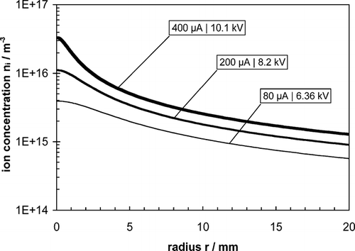
FIG. 3 Radial profiles of the electric field E₀(r) with and without the effect of space charge, calculated for two pairs of corona current and voltage in the core zone (L_core≈ 22 cm) of the charger (L_c = 24 cm; R_tube = 2 cm; R_wire = 0.05 cm; ion mobility Z_i = 1.4 · 10^{− 4} m²/Vs).

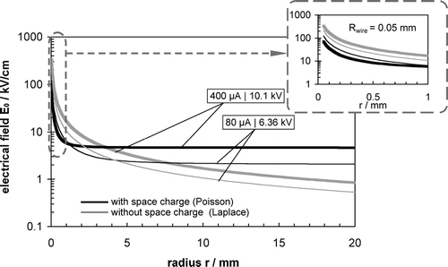
Zooming into the E-field near the corona electrode, Figure 3 shows different values of E₀ on the electrode surface (r_wire = 0.05 mm) for each set of calculations. This is not in agreement with the physically more reasonable assumption of a constant value around 150 kV/cm (the so-called Peek value; Hartmann 1984). The over-all error in the n_i-and E₀ averages for our experiments is estimated to be less than 3% (according to limiting case consideration of Jones et al. 1988: cases without unipolar space charge in corona zone and with maximum unipolar space charge in corona zone, respectively). This uncertainty is small compared to the error induced by the much less reliable ion mobility value Z_i, which can easily exceed 10% (e.g., Zebouddj and Hartmann 1999).

4. DETERMINATION OF THE MIXING STATE OF THE AEROSOL

The state of mixing of the aerosol was evaluated indirectly by comparing measured particle losses in the charger with model predictions. There are two theoretical limiting cases for particle deposition, one described by the Deutsch-model for the wire-tube ESP (Deutsch 1922), which assumes perfect radial particle mixing except for the boundary layer (the spatial analogy of a CSTR); the other case is for laminar plug flow with no particle mixing at all. As will be shown below, most experimental cases were found to be in excellent agreement with the Deutsch model. The aerosol was therefore sufficiently well mixed to assume that each particle had the same charging history described by the average electrical conditions calculated in the preceding section, and that the aerosol sampled at the charger outlet was representative for the entire charger, despite high particle losses.

For our application the original Deutsch model has to be modified with respect to the assumption that particles are fully charged at the charger inlet. This is no longer the case for nanoaerosols because charging happens much slower than in case of super-micron particles. Instead of the final charge level a certain average charge must be used (see below). The other assumptions made by Deutsch should hold equal or even better for nanoaerosols than for classical ESP-applications with large particles, namely that the flow is turbulent except in the boundary layer; that particles completely follow the gas flow; that particles in the laminar boundary layer will not reenter the turbulent core flow; and that within the laminar boundary layer particles move with the migration velocity w (average velocity ).

The modification of the Deutsch model formally refers only to the effective migration velocity (see below). We thus use the unchanged expressions for the size dependent loss T (T is the “grade efficiency”) derived by Deutsch:

where De is the non-dimensional Deutsch number

For a concentric cylindrical wire-tube geometry De becomes

with particle concentration c, surface of the deposition zone A, gas velocity u, tube radius R, and length of the (cylindrical) deposition zone L_dep.

For the second limiting case of a completely unmixed plug flow profile in a cylindrical tube, the loss function (Equation [12]) is derived in Appendix A:

For both limiting cases the effective migration velocity can be calculated from local radially averaged velocities (different values in axial direction; radial averaging of the particle charging conditions is admissible according to the central assumption of our experimental strategy; see Section 2). Thus, the effective migration velocity results as an overall average according to

A closer inspection of this equation reveals an intrinsic complication: evaluating the integral requires a-priori knowledge of the complete charging kinetic, q_P as a function of n· t, which is of course what we want to determine in the first place. In other words, proving the representativeness of our charge analysis requires validation of the particle transport hypothesis (particle losses), but validation of the transport hypothesis calls for representative charge measurements. We have therefore resorted to first measuring the charging kinetics, and then using it to verify the ideal mixing hypothesis a posteriori. If the loss data then match the Deutsch formula, we can conclude also that the charge measurements were representative. The plausibility of the mixing assumption is supported however by tube Reynolds numbers up to 7000 (Re = Ø_tube u _gas /ν).

In the next two sections, we will first discuss the charge measurements and compare them to charging theory from Part I. The justification of the mixing assumption via the particle transport hypothesis will be delayed to the end of the article.

5. EXPERIMENTAL CHARGE DATA VS. MODEL PREDICTIONS

This section presents charging data and compares them to theoretical predictions based on the models discussed in Part I. For the ion properties we use the widely accepted values Z₊ = 1.4 · 10^{− 4} m²/Vs, Z₋ = 1.9 · 10⁻⁴ m²/Vs, m₊ = 0.109 kg/mol, m₊ = 0.050 kg/mol (e.g., Adachi et al. 1985; Biskos et al. 2005).

5.1. Charging Kinetics

Figure 4 plots the measured average particle charge q_exit (measured at the charger outlet) versus the n· t product for five particle sizes between 30 and 100 nm, and compares these values to q_P as predicted by the Fuchs model for pure diffusion charging. The n·t product was varied by changing the corona intensity (i.e., current and voltage). The average E₀ values corresponding to each n· t are shown on the second ordinate. The second ordinate also underlines the fact that ion concentration and electric field are always coupled in this series of measurements.

FIG. 4 Average charge versus n· t product for different particle sizes and E-fields. Here n· t is varied only via the corona intensity and the E-field. Solid lines represent the Fuchs diffusion charging model (q_P); data points are measured values q_exit.

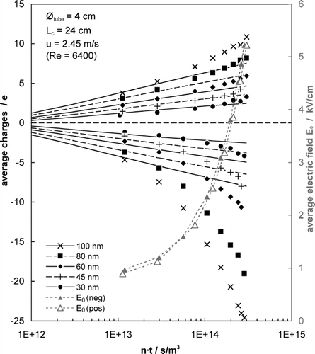
As expected from any model, the particles become more charged with increasing particle size and n· t value. For n· t values below 2· 10¹³ s/m³ (and corresponding electric fields of less than 1 kV/cm) the experimental points match the Fuchs prediction well, whereas above they begin to surpass the theoretical values significantly. The extent of this deviation differs with particle size and polarity and apparently becomes most pronounced for negative charging.

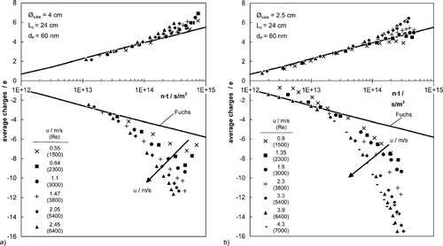
Figure 5 depicts similar data, however for only one particle size but different Reynolds numbers between 1500 and 7000, and hence also for different states of mixing. Re was varied with flow velocity and diameter of the charger (Figure 5a: Ø_tube = 4 cm and Figure 5b: Ø_tube = 2.5 cm, both with L_c = 24 cm). In all cases the deviations between measured and predicted charge increase above n· t ∼ 2· 10¹³ s/m³ (negative polarity) and 10¹⁴ s/m³ (positive polarity), respectively. For the larger tube diameter (4 cm) even the points corresponding to the lowest Reynolds number surpass the values predicted by diffusion charging theory, whereas for the thinner tube (2.5 cm) only the data with Re ≥ 5400 follow this trend. It is reasonable to assume that the aerosol was no longer well mixed at the lowest Re number. (This will of course be discussed in more detail in Section 6.)

FIG. 5 Average charge vs. n· t product for a fixed particle size of 60 nm and two different charger diameters (left 4 cm and right 2.5 cm). Here n· t is varied via the corona intensity and the flow velocity. Solid lines represent the Fuchs diffusion charging model (q_P); data points are measured values q_exit.

Next, we investigate the more central aspect of this article, namely, the effect of the electric field on charging. Figure 6 presents the charging kinetics of 60 nm aerosols obtained in various series of measurements with different geometries, and compares them with predictions by the 2-D limiting sphere model from Part I. We recall that this model now accounts for diffusion charging as well as the effect of the external field. In addition to the two charger geometries discussed so far, we have included further experiments with a shortened active corona wire (L_c = 5 cm, Ø_tube = 4 cm). The point in shortening the wire is that a higher field is required to achieve the same value of n· t. All data shown in Figure 6 were obtained at the high Reynolds number (Re = 6400), which can be considered the most “robust” condition in terms of mixing.

FIG. 6 Average charge vs. n· t product for 60 nm particles size at fixed flow Re number. Here n· t is varied via corona intensity. Thin lines are q_p/e calculated according to the field-diffusion charging model described in Part I; data points are measured values q_exit.

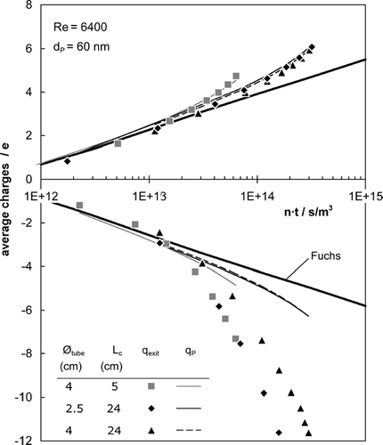
We see from Figure 6 that agreement between model and experiment is generally very good for positive charge carrier polarity. The theoretical treatment of the electric field presented in Part I apparently suffices to explain the deviations from the pure diffusion charging model (the thick “Fuchs line”), including also the more significant deviations of the shortened active corona zone (light gray symbols) which starts at lower n· t products.

In contrast to the positive corona polarity, the measurements obtained for negative polarity do not match up well with the new model, even though the agreement at lower n· t values (and thus lower corona intensities) is somewhat improved over pure diffusion charging. In the next section we shall try to show that the best explanation for this polarity specific discrepancy between data and model is to assume that free electrons participate in the charging process.

5.2. Arguments in Support of Charging by Free Electrons in the Negative Corona

For electropositive gases, charging by free electrons at STP is indeed known to be more efficient than by negative ions (e.g., Romay and Pui 1992a). In an electronegative atmosphere such as air however, the lifetime of free electrons is greatly reduced and ionic charging should be the dominating mechanism. There are only few and indirect reports of free electron charging in air, mainly from electrostatic precipitation experiments at elevated temperature by Penney and Lynch (1957), Crynack and Penney (1974), Jack et al. (1980), and Mizuno (1982). Their conclusions are based on experiments with particle sizes much larger than 100 nm, and by corona current-voltage analysis, by the observed grade efficiencies and partly by particle charge measurements. Direct experimental proof for electron charging in air is lacking, because there are no appropriate methods available.

Although our data offer no direct proof either that free electrons participate in the charging process, the following strong argument can be made in favor of this hypothesis: The two data sets for L_c = 24 cm & Ø_tube = 4 cm and L_c = 24 cm & Ø_tube = 2.5 cm are equal with regard to the positive charging kinetics, but differ significantly in the negative kinetics. Usually, only the passive corona zone is regarded for the charging process. Now, if free electrons contribute significantly to the particle charging (which is only to be expected for the negative corona), this must be limited to the electron-rich area close to the wire.

Even though the two chargers have different tube diameters, the absolute dimensions of the corona zones must be preserved, as the conditions close to the corona electrode (including the corona zone!) are equal with respect to wire diameter and field strength. However, for the thinner charger tube this area is more than twice as large compared to the total charger cross section. Hence, for the thinner tube free electron charging will make a stronger contribution to the total particle charge, and this is what the measurements actually show.

The above argument based on charging zones with more or less effective charge carriers (electrons vs. ions) can also be used to explain qualitatively, why the negative charging data in Figure 5a are so broadly fanned out for different aerosol flow rates through the charger, and why the data obtained at higher flow velocities show higher particle charges: the increased gas turbulence at higher flow rates may be responsible for pushing particles back more deeply into the electron rich zone near the wire. (This hydrodynamic transport is of course counteracted by the electrostatic forces, which limit this remixing close to the wire, due to the steep increase in the electric field—see Figure 3.)

5.3. Further Assessment of the Charging Model

In order to assess the predictive quality of the new model more thoroughly, further results are shown in Figure 7 and Figure 8 for the case of positive charging.

FIG. 7 Charging kinetics of 60 nm aerosol at fixed electric conditions; n· t-variation via charging time (sampling at different wall positions; lines calculated according to combined field and diffusion charging theory (model from Part I).

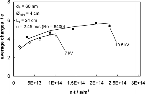
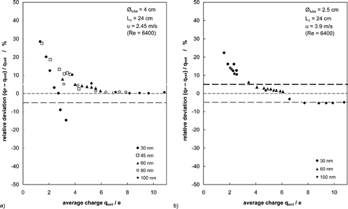
FIG. 8 Relative deviation between predicted (q_P) and measured (q_exit) charge versus measured particle charge for different particle size; n· t is varied only via the corona intensity. The model is calculated according to Part I. Gray dashed lines: range of estimated experimental error. (a) Large charger tube Ø_tube = 4 cm. (b) Small charger tube Ø_tube = 2.5 cm.

Figure 7 shows measurements for a fixed particle size of 60 nm, charging at a constant electric field and constant Re (i.e., constant hydrodynamic conditions, disregarding disturbances by sampling at the wall positions). n· t was varied only via the residence time in the charger. For the two cases at 7 kV and 10.5 kV (E₀≈ 2.5 kV/cm and 4.9 kV/cm, respectively) shown, there is very good agreement between experiment and theory.

For selected data from the same two charger geometries and at fixed Re, we have further plotted the percentage difference between measured and predicted charge (Figure 8a and Figure 8b). The data show both the effect of the actual charge level q_exit and the particle diameter on the deviations. The estimated experimental error of 5% is also indicated in the figure by parallel dashed lines.

Both diagrams show similar trends for smaller particles and lower charge levels, where the model tends to overpredict the charge. Above a level of about four elementary charges, model and data agree within the experimental error. Before analyzing Figure 8 in more detail it should be emphasized that all recording and processing of the experimental data was done and validated very carefully. Since the role of particle loss and sampling as a significant source of deviations can be ruled out—as discussed in the next section—the two major causes left to explain the remaining discrepancies must be related to the ion properties and/or the model itself.

The ion mass and mobility are required both for evaluating the charging conditions (requires electrical mobility Z_i) and as model input (requires Z_i, m_i). Reliable ion data for the own corona system will be difficult to obtain. On one hand currently available techniques based on average time-of-ion-flight measurements in a charger with triode arrangement (e.g., Hewitt-charger type; Kirsch and Zagnit'ko 1981 and 1990, Büscher et al. 1994) cannot be transferred to the given direct corona. (Conversely, a triode configuration makes it very hard to realize the desired high n· t products and electric fields with acceptable particle losses, and thus cannot be applied here.) On the other hand the alternative technique to gather ion data provided by time-of-flight ion mass spectrometers (TOFM, e.g., Nagato and Ogawa 1998) does not offer the time resolution required for the crucial lifetime window of ions (below 1 ms) in the given charger.

Unfortunately, the substantial computational effort required for model calculations makes it difficult to prepare a comprehensive sensitivity analysis with respect to ion mobility and ion mass. We performed a limited number of model computations (see Appendix of Part I, also Marquard 2006), where the ion parameters were varied. The result of a complete re-evaluation of the data from Figure 8a with higher ion mobility (increased by 20%) is given in Appendix B. It exemplarily illustrates that none of the checked parameter combinations produced a significantly better agreement between model and experiment than the one found above. As a matter of fact, it appears unlikely that better ion data would change much in the way of agreement between data and model and thus the commonly used ion data seem to be a very reasonable choice, since they applied well to the majority of cases considered here.

A further assessment of the model follows from looking at limitations in the model itself or its evaluation . As already discussed in Part I, these are first of all the same restrictions as for the original Fuchs model. In particular, neither model accounts for the ion velocity distribution, which becomes increasingly important for smaller and/or higher charged particles and a correspondingly higher electrostatic potential barrier. Therefore all Fuchs-based models tend to underestimate the particle charge below about 30 nm or even larger particles with higher charge levels (Filippov 1993). Figure 8 indeed reflects such an expected decrease of predicted charge for each particle size with increasing charge level; surprisingly however, the weakly charged 30 nm particles are overestimated by up to 30%, whereas for higher charges the predictions approach the measured values.

It may again appear obvious to blame incorrect ion data (see above) or flaws in the calculation of the ion-particle collision coefficients α for the observed discrepancy in the 30 nm (and 45 nm) data. However, the general procedure for calculating α was assessed in Part I and found to be reasonably good. With respect to the experiments with particle sizes below 45 nm the over estimation of the weakly charged particles cannot be explained by the neglect of ion velocity distribution. From the sensitivity analysis (Appendix Part I) it is known that possible effects of incorrect ion data on the model are quite independent of particle size, which also is contrary to our findings.

We were able to identify only one potential error source which is size-dependent, which is reduced by increasing particle charge, and could lead to some degree of overprediction of the charge for small and weakly charged particles: The model calculations were based on a simplified (but very common) expression for the image potential, which causes the resulting potential barriers to be lower than in case of the exact expression by Lushnikov and Kulmala (2005). As mentioned in Part I, all model calculations here were carried out with the simpler image force approximation, and the impact of this simplification on the charging results could not be checked (because the specific integral in Equation [2], Part I, cannot be implemented into a Comsol 3.2 scheme).

6. ASSESSMENT OF THE EFFECT OF PARTICLE LOSSES ON CHARGING DATA

The assessment of particle losses is necessary in order to legitimate the procedure of evaluating the charging conditions. The functional dependence of particle losses on the residence time in the charger will be used as the key argument to support the complete mixing hypothesis, which is in turn required for “representative sampling.” (In this work the term “representative sampling” is used for the case that the analyzed particles have known charging histories.) This legitimacy is all the more important, because it allows to base the charge determination on an average value derived from sampling a significant portion of the channel cross section, while the ion concentration inside the charger varies radially by up to one order of magnitude (Figure 2).

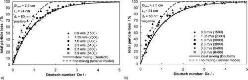
In the following, we compare the measured particle losses (y-axis) for positive and negative corona with the two limiting case models for ideal mixing and no mixing respectively (see Section 4). The Deutsch numbers (x-axis) are based on the measured charging kinetics from Section 5 and calculated according to Equations (11) and (13). We use data for a fixed particle size (60 nm) and the two charger diameters of 2.5 and 4 cm, as shown in Figure 9a, Figure 9b and Figure 10a, Figure 10b. The different symbols refer to measurements at different flow velocities.

FIG. 9 Particle losses in the charger for positive and negative corona, compared to theoretical limiting cases for complete radial mixing (Deutsch model) and laminar flow (charger tube Ø_tube = 4 cm). (a) Positive and (b) negative polarity.

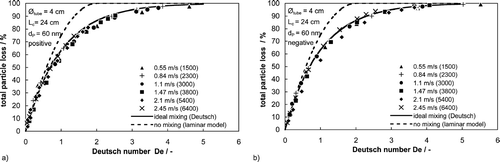
FIG. 10 Particle losses in the charger for positive and negative corona, compared to theoretical limiting cases for complete radial mixing (Deutsch model) and laminar flow (charger tube Ø_tube = 2.5 cm). (a) Positive and (b) negative polarity.

In case of the larger diameter charger (Figure 9) all measurements fall closely around the Deutsch curve with surprisingly low scattering for both positive and negative charging. (Scattering was greatly reduced by sampling from Port 2 instead of Port 1 in Figure 1.) Complete radial particle mixing can therefore be assumed for all gas flows, even for seemingly laminar conditions. Obviously, the additional turbulence induced by ion winds inside the charging region contributed to the remixing process. With regard to the great similarity of agreement of positive and negative data it has to be noted again that here, no charging model but measured charging kinetics are used. This allows for the validation of the Deutsch assumptions independent of any charging model assumptions.

For the thinner charger (Figure 10), only the measurements at the highest Reynolds number (Re = 6400) follow the Deutsch curve for complete mixing, while the others tend progressively toward the laminar curve. The series up to Re = 3000 even lie partially to the left of the curve of the laminar case—outside the reasonable domain. This means, that the charge measurements obtained at those lower flow rates were not completely representative for the comparison with the model, and that the lost particles presumably carried higher charges than the particles analyzed. This finding agrees well with what was discussed in Section 5, Figure 5b concerning the charging kinetics. Therefore only the data at high Reynolds numbers were used for quantitative comparisons with the charging model.

A final analysis of the data concerns the relationship between attained particle charge versus particle losses in the charger used here. Marquard et al. (2006a, 2006b) have shown that this is an important practical criterion in evaluating effective chargers. It was pointed out there in particular, that an AC electric field is not as beneficial as often believed for a good compromise between efficient charging and low losses. Furthermore, rapid charging (i.e., high ion concentrations and low residence times) tends to reduce the particle losses for a given particle charge. Here, this conclusion can be refined and extended with selected data for the lowest and the highest Reynolds number investigated (Figure 11).

FIG. 11 Particle losses versus particle charge attained in the charger for two series with low and high Reynolds number.

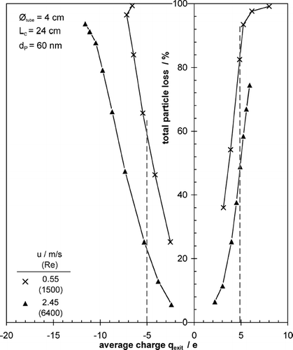
The diagram clearly illustrates the advantage of a residence time reduction (here by a factor of 4.5) at a desired level of charge. For equal charging results, higher Re numbers support lower particle losses, which however is observed to a different extent for both polarities. This means not only the residence time, but also the flow turbulence significantly affects the charge loss relation. This more subtle point can be made when comparing the two polarities: One sees that the curves on the positive side are closer together than at the negative side, e.g., at q_exit = ± 5 e which is marked in the figure. As concluded above, the degree of flow turbulence causes the depth of particle penetration into the electron enriched volume close to the corona.

Thus, greater loss reduction potential for a “well-mixed” charger operated with negative polarity comes into play with the presence of free electrons as discussed earlier.

7. CONCLUSIONS AND OUTLOOK

A new strategy has been applied to the investigation of combined field and diffusion charging of sub-100 nm aerosols under conditions of intense charging. The experiments cover n· t products up to 5· 10¹⁴ s/m³ and average electric fields up to 5.5 kV/cm. The average particle charge and particle losses measured in a wire-tube corona charger were compared to model calculations for charging and particle transport in the charger.

The functional relationship between measured particle losses and Deutsch number leads to the conclusion that the strategy of using a well-mixed and turbulent charger is effective in assuring representative data and a well-defined charging environment.

The charge data were used to validate a 2-dimensional limiting-sphere model for combined charging by diffusion and an external electric field. It is shown that agreement between model calculations and experiments is very good for the case of positive charging. At the same time, these experiments demonstrate the relevance of an external electric field for particle charging by ions in the transition regime.

Further refinement of the model (e.g., inclusions of the ion velocity distribution, use of the exact image potential) should improve matching with experimental data also for smaller particles (d_P ≤ 45 nm) and lower charge levels (q_P ≤ 4 e).

The existence of aerosol charging by free electrons in case of a negative corona polarity at ambient temperature has been inferred. This finding brings electron charging into play as purposeful mechanism for new and simple aerosol chargers with low particle losses. In order to deepen the understandings, this point could be investigated further by additional experiments with gas atmospheres containing different amounts of electronegative and electropositive gas species. Finally, the model could be extended for the case of electron charging. For that purpose well-known work on aerosol charging by free electrons (e.g., Romay and Pui 1992a; Wiedensohler and Fissan 1988) might provide useful support.

It would be helpful to develop a simple empirical formula on the basis of the model described in Part I, in order to shorten the computational process of charge prediction in the transition regime. As shown in Part I, the according continuum regime model by Lawless (1996) could serve for that goal at high n· t-products (n· t > 10¹³ s/m³), despite physical inconsistencies.

Whether the new 2-D limiting sphere model (described in Part I) or the Lawless model are better able to describe low intensity charging in the transition regime, cannot be proven with the data presented here, since it is hard to establish n· t-products < 10¹² s/m³ with the given direct corona charger. (Experiments with voltages close to the corona onset result in unstable and non-uniform corona currents accompanied with low electric fields; higher throughputs and shorter corona lengths have their own practical limitations.)

NOMENCLATURE

Greek Symbols

ϵ	=	permittivity, C/Vm
ϵP, ϵr	=	specific permittivity of particle and gas, respectively—
ϵ0	=	dielectric constant, 8.854· 10− 12 C/Vm
ϕ	=	electrostatic potential, V
ν	=	kinematic viscosity, m2/s
ρ	=	space charge density, C/m3
σg	=	geometric standard deviation,—

Latin Symbols

A	=	cross section area, m2
c	=	particle concentration, 1/m3
C	=	slip correction,—
ci	=	thermal ion velocity, m/s
c	=	particle concentration, 1/m3
De	=	Deutsch number,—
Di	=	diffusion coefficient of ions, m2/s
dP	=	particle diameter, m
e	=	elementary charge unit, 1.602· 10− 19 C
E	=	electric field, V/m
E0	=	external electric field (compare Part I), V/m
j i	=	ion current density, A/m2
k	=	Boltzmann constant, 1.381· 10− 23 J/K
l	=	length coordinate, m
L	=	length of charging chamber, m
Ldep	=	length of deposition zone, m
loss	=	particle loss,—
m	=	molar mass, kg/mol
n	=	concentration, 1/m3
N	=	particle rate, 1/s
n· t	=	product of ion concentration and charging time, s/m3
Ø	=	diameter, m
Q	=	flow rate, m3/s
qexit	=	average particle charge measured at charger outlet, C
qP	=	theoretical average particle charge, C
r	=	radial coordinate, m
r*	=	critical radial inlet position, m
r, R	=	radius, m
Re	=	Reynolds number,—
t	=	time, s
T	=	temperature, K
T	=	loss function (grade efficiency),—
u	=	gas velocity, m/s
V	=	volume, m3
w	=	migration velocity, m/s
x	=	length coordinate, m
Zi	=	ion mobility, m2/Vs

Subscripts

c	=	corona
core	=	core zone
dep	=	deposition zone
i	=	ion
P	=	particle
wire	=	corona wire
tube	=	charger tube wall
in	=	at inlet
out	=	at outlet

Abbreviations

PVC	=	poly vinyl chloride
ESP	=	electrostatic precipitator
FEM	=	finite element method
CSTR	=	continuously stirred tank reactor
TOFM	=	time of flight mass spectrometer
PDE	=	partial differential equation
FCE	=	faraday cup electrometer
DMA	=	differential mobility analyzer
CPC	=	condensation particle counter
DEHS	=	di-ethyl hexyl sebacate

APPENDIX A: LOSS PREDICTION OF PARTICLES IN A WIRE-TUBE ESP FOR LAMINAR FLOW WITHOUT PARTICLE REMIXING

The considered case implies ideal gas plug flow with non-crossing streamlines in a (concentric) wire-tube arrangement (length L and tube radius R). The aerosol particles are uniformly distributed at the inlet. They follow the gas without inertia in flow direction (velocity u). Perpendicular to the gas flow the charged particles move with the migration velocity w towards the wall of the tube. All particles starting outside an inner cross section with the critical radius r* will be deposited at the wall; all particles starting at r < r* will penetrate through the charger.

The loss (i.e., grade efficiency) is then given by the area ratio of the outer annular gap (r* < r < R_tube) to the total cross section.

Equating the residence times in flow direction and in wall direction gives the critical radius r* :

Inserting (A-2) together with the Deutsch number (Equation [11]) into (A-1) gives the expression in demand (Equation [12])

APPENDIX B: RE-EVALUATION OF EXPERIMENTAL DATA AND MODEL PREDICTIONS WITH DIFFERENT ION MOBILITY DATA

In Figure 12 the experiments shown in Figure 8a are again compared to model predictions, now assuming 20% higher ion mobilities (Z_i = 1.68· 10^{− 4} V/m²s; molar ion mass kept at M_i = 0.109 kg/mol) for determination of the charging conditions and for the model calculations.

FIG. 12 Relative deviation between predicted (q_P) and measured (q_exit) charge vs. measured particle charge for different particle size; n· t is varied only via the corona intensity. Evaluation contrary to Figure 8a here with an ion mobility of Z_i = 1.68 m²/Vs. Gray dashed lines: range of estimated experimental error.

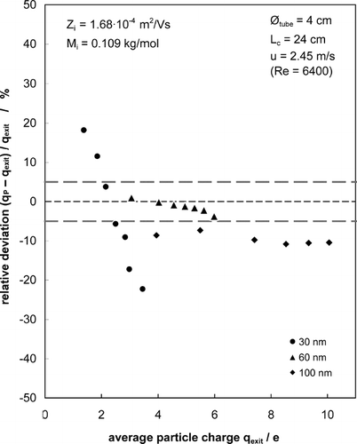
Compared to Figure 8a the agreement between measured and predicted data is worse. The higher mobility reduces the predicted values nearly independent of particle size, even though one might expect increased charging (see Figure 11, Appendix, Part I). This effect is in fact included in the result, but it is obviously overcompensated by the decrease of average ion concentration (i.e., lower n· t-product) due to faster moving ions at constant corona current.

Acknowledgments

Financial support by the German Science Foundation Deutsche Forschungsgesellschaft (DFG) and by the Elstatik foundation of Sylvia & Günter Lüttgens is gratefully acknowledged.

REFERENCES

- Adachi , M. , Kousaka , Y. and Okuyama , K. 1985 . Unipolar and Bipolar Diffusion Charging of Ultrafine Aerosol Particles . J. Aerosol Sci. , 16 : 109 – 123 .
- Biskos , G. , Reavell , K. and Collings , N. 2005a . Unipolar Diffusion Charging of Aerosol Particles in the Transition Regime . J. Aerosol Sci. , 36 : 247 – 265 .
- Brown , G. 2004 . The Physics and Technology of Ion Sources , Weinheim : John Wiley .
- Buescher , P. , Schmidt-Ott , A. and Wiedensohler , A. 1994 . Performance of a Unipolar “Square Wave” Diffusion Charger with Variable nt-Product . Journal of Aerosol Science , 25 : 651 – 663 .
- Capitelli , M. 2000 . Plasma Kinetics in Atmospheric Gases , Heidelberg : Springer .
- Crynack , R. R. and Penney , G. W. 1974 . Charging of Fine Particles in Negative Corona Near Sparkover . IEEE Transactions on Industry Applications , IA-10 : 524 – 530 .
- Deutsch , W. 1922 . Bewegung und Ladung der Elektrizitätsträger im Zylinderkondensator . Annalen der Physik [IV] , 68 : 335 – 344 .
- Gallimberti , I. 1979 . The Mechanism of the Long Spark Formation . Journal de Physique , Colloque C7, Supplément 7, Tome 40, C7-194-250
- Gallimberti , I. 1998 . Recent Advancements in the Physical Modelling of Electrostatic Precipitators . Journal of Electrostatics , 43 : 219 – 247 .
- Hartmann , G. 1984 . Theoretical Evaluation of Peek's Law . IEEE Transactions on Industry Applications , IA-20 : 1647 – 1651 .
- Hippler , R. , Pfau , S. , Schmidt , M. and Schoenbach , K. H. 2001 . Low Temperature Plasma Physics , Weinheim : John Wiley .
- Jack , R. , McDonald , J. R. , Anderson , M. H. , Mosley , R. B. and Sparks , L. E. 1980 . Charge Measurements on Individual Particles Exiting Laboratory Precipitators with Positive and Negative Corona at Various Temperatures . J. Appl. Phys. , 51 : 3632 – 3643 .
- Jones , J. E. 1992 . On the Drift of Gaseous Ions . J. Electrostat. , 27 : 283 – 318 .
- Jones , J. E. , Dupuy , J. , Schreiber , G. O. S. and Waters , R. T. 1988 . Boundary Conditions for the Positive Direct-Current Corona in a Coaxial System . J. Physics D: Applied Physics , 21 : 322 – 333 .
- Kaptzov , N. A. 1947 . Elektricheskie Invulentiia v Gazakh I Vakuumme . OGIZ Moskau , : 587 – 630 .
- Kirsch , A. A. and Zagnit'ko , A. V. 1981 . Diffusion Charging of Submicrometer Aerosol Particles by Unipolar Ions . J. Coll. Interface Sci. , 80 : 111 – 117 .
- Kirsch , A. A. and Zagnit'ko , A. V. 1990 . Field Charging of Fine Aerosol Particles by Unipolar Ions . Aerosol Sci. Technol. , 12 : 465 – 470 .
- Lawless , P. A. 1996 . Particle Charging Bounds, Symmetry Relations and an Analytic Rate Model for the Continuum Regime . J. Aerosol Sci. , 27 : 191 – 215 .
- Lushnikov , A. A. and Kulmala , M. 2005 . A Kinetic Theory of Particle Charging in the Free-Molecule Regime . J. Aerosol Sci. , 36 : 1069 – 1088 .
- Marquard , A. 2006 . Unipolare Aufladung nanoskaliger Aerosolpartikeln bei hohen Ladungsträgerdichten , Dissertation Universität Karlsruhe (TH) .
- Marquard , A. , Kasper , M. , Meyer , J. and Kasper , G. 2005 . Nanoparticle Charging Efficiencies and Related Charging Conditions in a Wire-Tube ESP at DC Energization . J. Electrostat. , 63 : 693 – 698 .
- Marquard , A. , Meyer , J. and Kasper , G. 2006a . Characterization of Unipolar Electrical Aerosol Chargers—Part I: A Review of Charger Performance Criteria . J. Aerosol Sci. , 37 : 1052 – 1068 .
- Marquard , A. , Meyer , J. and Kasper , G. 2006b . Characterization of Unipolar Electrical Aerosol Chargers—Part II: Application of Comparison Criteria to Various Types of Nanoaerosol Charging Devices . J. Aerosol Sci. , 37 : 1069 – 1080 .
- Mizuno , A. Review of Particle Charging Research . Proceedings of the 1st International Conference on Electrostatic Precipitation . Pittsburgh. pp. 304 – 325 .
- Mohnen , V. A. Formation, Nature and Mobility of Ions of Atmospheric Importance . Proceedings of the 5th International Conference on Atmospheric Electricity . Garmisch-Patenkirchen. pp. 1 – 17 .
- Nagato , K. and Ogawa , T. 1998 . Evolution of Tropospheric Ions Observed by an Ion Mobility Spectrometer with a Drift Tube . Journal of Geophysical Research , 103 : 13.912 – 13.925 .
- Peek , F. W. 1929 . Dielectric Phenomena in H. V. Engineering , 25 – 80 . McGraw Hill .
- Penney , G. W. and Lynch , R. D. 1957 . Measurements of Charge Imparted to Fine Particles by a Corona Discharge . AIEE Transactions , 76 : 294 – 299 .
- Pui , D. Y. H. , Fruin , S. and McMurry , P. H. 1988 . Unipolar Diffusion Charging of Ultrafine Aerosols . Aerosol Sci. Technol. , 8 : 173 – 187 .
- Romay , F. J. and Pui , D. Y. H. 1992 . On the Combination Coefficient of Positive Ions with Ultrafine Neutral Particles in the Transition and Free-Molecule Regimes . Aerosol Sci. Technol. , 17 : 134 – 137 .
- Romay , F. J. and Pui , D. Y. H. 1992a . Free Electron Charging of Ultrafine Aerosol Particles . J. Aerosol Sci. , 23 : 679 – 692 .
- Sheng , J. N. , Yan , Z. , Qin , B. L. and Gela , G. 1988 . DC Ion Flow Fields: Uniqueness of Solution and Application of the Charge Simulation Method . Journal of the Franklin Institute , 325 : 315 – 334 .
- Sigmond , R. S. 1986 . The Unipolar Space Charge Flow Problem . J. Electrostat. , 18 : 249 – 272 .
- Townsend . 1915 . Electricity in Gases , Berkeley : University of California Press .
- Wiedensohler , A. and Fissan , H. J. 1988 . Aerosol Charging in High Purity Gases . J. Aerosol Sci. , 19 : 867 – 870 .
- Zebboudj , Y. and Hartmann , G. 1999 . Current and Electric Field Measurements in Coaxial System During the Positive DC Corona in Humid Air . Euro. Phys. J. Appl. Phys. , 7 : 167 – 176 .