Simultaneous Measurements of PM₁₀ and PM₁ using a single TEOM^#

Abstract

A time sharing, sequential scanning inlet system has been developed for a tapered element oscillating microbalance (TEOM) particulate matter (PM) mass measurement instrument, allowing quasi simultaneous measurement of ambient PM₁₀ and PM₁. Compared to running two separate instruments this approach eliminates systematic biases between the PM₁₀ and PM₁ data due to slightly different response functions of separate instruments. Furthermore, this approach reduces the costs of the measurements considerably. The system has been successfully tested during the winter 2005/2006 in Zurich, Switzerland and 24-hour average data have been compared to ambient concentrations measured with reference high volume sampler systems of the Swiss national air pollution monitoring network (NABEL) showing an excellent correlation. We demonstrate the use of our instrument for characterizing PM by showing the significant differences between PM₁₀ and PM₁ in their respective diurnal variation patterns as well as the increase in their concentrations during events of air stagnation.

INTRODUCTION

Recently, Ayers (2004) suggested the use of a single Tapered Element Oscillating Microbalance (TEOM) (Patashnick and Rupprecht 1991), with sequential scanning across separate PM₁₀, PM_2.5, and PM₁ size selective inlets for determining three particle mass measures. He showed by numerically degrading the resolution of a time series of TEOM data measured in Melbourne, Australia in December 2001, that little was lost for that data set in terms of accuracy and precision of hourly and daily data when compared to data obtained with three separate instruments. He concluded that the fractional error for the hourly averages of an instrument with two time shared inlets is mostly between ± 3%. The errors for 24 hours averages in the numerical study stayed below ± 1% in all but one day of the eight–day time series considered. Besides saving costs this approach would eliminate systematic biases between different instruments, providing the additional advantage that the ratios of particle mass measures of different sizes should of high accuracy, even when only averaged over short periods of time. Such consistent data may for example help in characterizing air masses of different origins or allow the study of the aging.

Here, we report on a realization of this idea for two size selective inlets, PM₁₀ and PM₁, detailing the mechanical design, electronic control and data processing. The instrument was tested in the winter 2005/2006 in Zurich. This time period was characterized by several events of air stagnation affecting the whole Swiss plateau with PM₁₀ concentrations exceeding the national standard for air quality of Switzerland (50 μ g/m³, 24-hour average with no more than one exceedence per year). Comparisons with reference measurements were possible, allowing us first to characterize and verify the operational concept of the instrument, and second to illustrate the feasibility of the time sharing approach by analyzing the diurnal variation and the gradual increase in PM concentration during the stagnation events.

MECHANICAL DESIGN

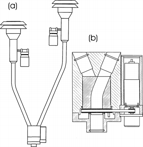
To facilitate sequential scanning we built a special motor driven valve as shown in Figure 1. It basically consists of a gear-belt-driven cylinder with an inner curved smooth cylindrical groove to avoid particle deposition within the valve. The cylinder is assembled from two halves with a curved groove milled into each half. It has a length of 90 millimeters and a diameter of 70 millimeters. By rotating the cylinder 180^ˆ the flow is switched from one inlet to the other. A switching period lasts for about 7 seconds, meaning that there are flow-switching transients during this time which have to be taken into account by the data processing, see below. Two electrical switches are mounted to the cylinder so that one of them closes when the opening is aligned with either input. They are wired in series with the DC motor driving the valve, thus the motor stops automatically when the opening is aligned to the other inlet. The whole valve can be simply mounted on one end onto the inlet tube of the TEOM and two different standard size selective inlets with their tubing can be mounted on the two inlets of the valve as shown in Figure 1. Sealing is achieved with O-rings, both between the inlets and the block holding the cylinder, and between the block and the inlet tube of the TEOM. These sealings were all leak tested. To avoid crosstalk between the two inlets, the upper surface of the cylinder and its counterpart are made from precision machined aluminum that is hardened by anodization. The remaining gap thickness is, at most, of the order of a few micrometers, which will lead to a crosstalk flow rate substantially below 1:10,000. The resulting crosstalk error in mass concentration is negligible compared to overall measurement error. We used a standard PM₁₀ inlet (D50 particle cut point at 10 μ m, Rupprecht & Patashnick Co.) and a PM₁ inlet with pre-separation of PM₁₀ followed by a sharp cut cyclone inlet (Rupprecht & Patashnick Co.).

FIG. 1 Schematic of the setup: (a) Overview of the valve together with the size selective inlets. (b) More detailed view of the valve with the attached motor.

ELECTRONIC CONTROL AND DATA PROCESSING

A personal computer with a graphical programming environment (Agilent VEE) is used to control the scanning valve and read in the raw frequency data via the serial interface of the TEOM control unit. The digital outputs of the TEOM control unit toggle between the inlets by switching a relay every 5 minutes which bypasses the mechanical switches inside the valve for about 1 s. This way the DC Motor runs until it is stopped by the next mechanical switch, selecting the other inlet. The aerosol mass weighting principle used in the TEOM is described by Patashnick (1975), Patashnick and Rupprecht (1979), and Patashnick and Rupprecht (1991). In brief, a hollow tube with a replaceable filter installed at one end is clamped on the other end and oscillates precisely at its natural frequency. The flow through the filter and the amplitude of the oscillation are both maintained by electronic feedback. Any particles collected on the filter shifts the natural frequency of the system from which the deposited mass can be determined. The inlet above the mass transducer and the filter are heated to 50°C to reduce biases due to condensation or evaporation of water from the particles (Patashnick and Rupprecht 1991), that could otherwise lead to substantial noise in the mass signal. This heating, however, also causes loss of semivolatile material (see discussion below).

We sample the raw frequency data every 2 seconds and average them over 10 seconds to reduce noise. Linear regression is used to determine the frequency change within each 5-minute time interval, from which the corresponding PM mass concentrations are calculated using the factory calibrated “spring” constant of the TEOM and the measured flow rates. The valve then switches to the other inlet and the procedure is repeated.

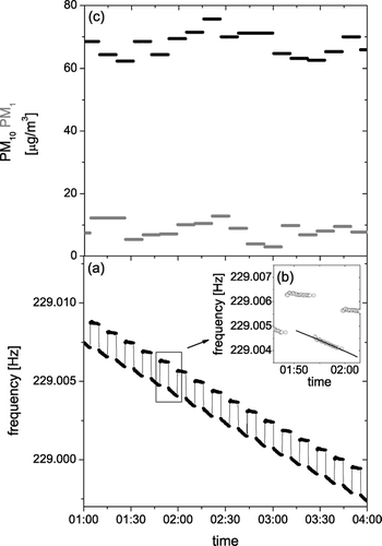
Figure 2 shows an example of the raw data and the corresponding mass concentrations. The dependence on the selected inlet is clearly visible as a difference in the frequency change with time between successive 5-minute intervals. From Figure 2b a small offset immediately after switching the inlets can be recognized, probably due to a slight difference in total pressure at the microbalance with a PM₁₀ inlet compared to a PM₁ inlet while maintaining the absolute flow rate. The TEOM always measures a higher absolute frequency with the PM₁ inlet than with the PM₁₀ inlet. We eliminate any effect of this offset on the mass retrieval by excluding the first six data points after switching when performing the linear regression calculation.

FIG. 2 General principle of operation. (a) Raw frequency data of the TEOM for a period of 3 hours on January 14, 2006. Clearly visible are the 5-minute switching cycles and the different slopes of frequency change with time for the different inlets, see text. (b) A 15-minute cutout of the data of panel (a) illustrating the linear regression used to determine the frequency change with time. (c) Masses for PM₁ (grey) and PM₁₀ (black) retrieved from the data of panel (a).

COMPARISON WITH REFERENCE DATA

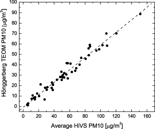
During the winter 2005/2006 the instrument was placed in a container together with instruments for measuring gas phase air pollutant concentrations and meteorological parameters on a hill 110 meters above the city center of Zurich and close to its border (at the campus of ETH at Hönggerberg). The site sits in a meadow approximately 150 meters away from a forest and about 500 meters from the nearest street. The 2005/2006 winter was characterized by several stagnation events with strong inversions affecting the whole Swiss plateau and allowing the accumulation of air pollutants to concentrations exceeding the Swiss air quality limits for PM₁₀ and NO₂. Figure 3 shows the daily averaged PM₁₀ concentrations measured at a number of stations in Zurich and its vicinity from both high volume sampler reference instruments and the PM₁₀ data with our inlet–time–sharing instrument. The reference stations use a Digitel DAH-80 High Volume Sampler at a flow rate of 30 m³·h⁻¹ with a single stage impactor for measuring PM₁₀ and a double stage impactor for measuring PM₁. Clearly there is a strong correlation between hi-vol measurements at all stations and our measurements, but in addition the reference instruments at all stations except Härkingen which is located in immediate vicinity of a national motorway show almost identical concentrations both during stagnation periods and during cleaner periods. This allows us to compare the average concentration measured with the reference method at all stations (excluding Härkingen) with our measurements as shown in Figure 4. In agreement with Ayers (2004), the present analysis demonstrates the time-sharing concept does not limit precision, as indicated by the high correlation (R² = 0.96) of the datasets. The deviation from the averaged concentrations of all reference stations to our measurement does not exceed that of any individual station from that average. Reduced major axis regression analysis (Ayers 2001; Bohonak and van der Linde 2004) reveals a slope of 0.61showing substantial loss of our PM₁₀ mass compared to that determined with the reference method. The small slope is not unexpected since we used the TEOM in its basic heated configuration with the temperature of the filter and inlet of the microbalance heated to 50°C. Numerous previous studies have observed this artifact (especially pronounced during the winter months) and attributed it to the loss of volatile and semivolatile components of the PM, particularly ammonium nitrate, numerous organics compounds and particle–bound water. For example, in a long-term study for urban and rural New York State locations for the winter months, Schwab et al. (2004) find an average slope of 0.66, with variation ranging from 0.58 to 0.82 depending on specific month and location for PM_2.5 standard TEOM data. Charron et al. (2004) find a slope of 0.52 for a rural UK site for PM₁₀ TEOM compared to PM₁₀ gravimetric (Partisol) data, and show that adding calculated particulate ammonium nitrate to the PM₁₀ TEOM improves the relationship significantly. Similar results were obtained by Chung et al. (2001) during the winter in California, yielding a slope of only 0.37 between PM₁₀ TEOM and reference high volume PM₁₀. They also concluded that the difference between both methods is due mainly to the loss of volatile ammonium nitrate. Cyrys et al. (2001) finds a slope of 0.69 for spring time PM_2.5 data in Germany. When they heated the reference high volume sampler to 50°C they found the same losses occur for it and the 50°C TEOM.

FIG. 3 Daily averaged concentrations of PM₁₀ (high volume sampler reference measurements) for a number of Swiss plateau stations (open symbols, dotted lines) during winter 2005/2006. Left scale:circles—Zurich-Stampfenbachstrasse, squares—Tänikon, upward triangles—Dübendorf (EMPA), downward triangles—Zurich-Kaserne, diamonds—Härkingen, rightward triangles—Opfikon. Right scale: daily averaged PM₁₀ concentrations measured with the inlet time sharing instrument at Zurich-Hönggerberg (filled circles, solid line). Corrosion of the original switches of the instrument caused some extensive maintenance time, being the cause for the data gaps in our series.

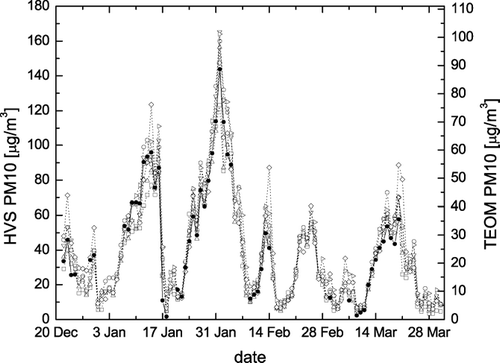
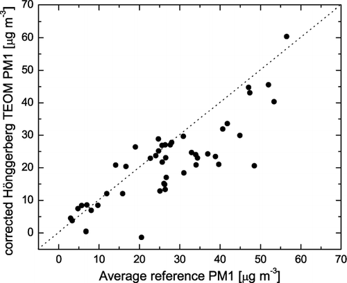
FIG. 4 Scatter plot of 24-h PM₁₀ mean concentrations of our measurements versus the average 24-h PM₁₀ mean concentrations of the five Swiss plateau reference stations shown in Figure 3 without the Härkingen data. Reduced major axis regression analysis leads to an offset of (–0.9 ± 1.0) μ g/m³ and a slope of (0.61 ± 0.02) with a high correlation (R² = 0.96).

Comparing our PM₁ data to those from the reference stations is not as straightforward as in the case of PM₁₀ because fewer reference stations are available for data comparison. Reduced major axis regression analysis yields a slope of (0.55 ± 0.05) and an offset of (−3.2 ± 1.4 μ g/m³) for PM₁ with a smaller correlation than in the PM₁₀ comparison (R² = 0.67). Since the slope is not significantly smaller with PM₁ compared to PM₁₀, we corrected our raw PM₁ data with the factor derived above for PM₁₀ and compare it to the average of two PM₁ data sets measured in the framework of the Swiss national air quality network (NABEL) at Basel-Binningen and Härkingen. Figure 5 shows this comparison. While about half the data scatter closely around the 1:1 ratio line, the other half of our data are approximately 10 μ g/m³ lower than those of the reference station, showing no systematic lower slope. At this time we can only speculate whether this is due to generally higher concentrations at the Basel and Härkingen sites compared to our less exposed site or due to different compositions on certain days of PM₁ compared to the PM₁₀ we used to derive the correction factor for volatile losses, or both. For example, consider the data point showing negative mass (–1.3 μ g/m³) at our site and 20.5 μ g/m³ average at the reference station. It dates from January 17, 2006 (see Figure 3), when a front passed our station after a prolonged stagnation period. The air was very clean on this day at our site but considerable mass had been collected on the filter during the days preceding the front. First, this shows the negative artifact due to evaporation of accumulated mass from the filter. Second, the breakup of the stagnation might have occurred at slightly different times at the different sites leading to a poor correlation.

FIG. 5 Scatter plot of 24-h PM₁ mean concentrations of our measurements versus the average of two reference PM₁ datasets measured at Basel-Binnigen and Härkingen. The dotted line marks the 1:1 ratio.

Our overall conclusion based on these observations is that the TEOM with time sharing inlets works as intended, namely as two instruments with separate inlets would do, without introducing additional artifacts.

STAGNATION EVENTS IN WINTER 2005/2006

It is obvious from Figure 3 that a wide-spread, regional pollution of PM over the Swiss plateau existed for extended periods of several days each during winter 2005/2006, resulting in rather homogeneous PM concentrations independent of the specific site location. In the following we discuss the diurnal variation as well as the gradual increase in PM concentrations at our site in order to illustrate the utility of data from the inlet-time-sharing TEOM instrument.

Figure 6 shows the diurnal variation at the Hönggerberg site. Panel (a) shows that PM₁₀ and PM₁ do not follow a similar pattern, but are distinctly different. This contrasts to the trends observed during winter 2000/2001 in Austria (Gomišček et al. 2004). The PM₁₀ concentrations show high values during night and lower values during the day with a decrease by roughly 10% (∼ 5 μ g/m³) at early afternoon compared to the maximum night concentrations. The daytime evolution follows approximately the inverse pattern of the solar radiation, but perturbed by a morning peak that coincides with the peak in NO _x at the same site. This behavior has been observed in Zurich previously for PM₁₀ (Fisseha et al. 2006) and can be qualitatively understood: primary pollutants are diluted by the increase in the height of the stagnation layer during the day. There is superimposed on this diurnal variation the emissions peak in the morning and, to a lesser degree, one in the early evening hours. Both emission peaks may arrive at our site slightly late because of its elevated location at the city border.

FIG. 6 Average diurnal variation of key meteorological parameters and pollution concentrations (hourly averages) at Hönggerberg during the period shown in Figure 3(a). Particulate matter concentration:solid circles—PM₁₀ concentrations corrected for loss of volatile compounds by means of the functional dependence given in Figure 4, solid squares—PM₁ concentrations corrected with the same function; open circles—for comparison PM₁₀ concentrations at Härkingen averaged over the same time period; open squares—corresponding PM₁ concentrations at Härkingen. These half hour averaged data measured with either a beta-gauge or TEOM instrument are linked to the gravimetric reference data as described by Gehrig et al. (2005). (b) NO _x concentration. (c) Left axis (solid circles)—temperature evolution during the day; right axis (line)—corresponding solar radiation.

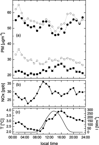
Interestingly, the PM₁ concentrations do not follow this pattern at all. Instead, they behave almost inversely, following the evolution of the temperature with a maximum in the early afternoon. There is no clearly discernible morning peak. Such diurnal variation may be attributed to secondary pollutants whose concentrations increase during daytime because a greater volume of the atmosphere is available to produce secondary material that can reach the ground level as particulate and possibly some photochemical reactions increasing the secondary material as well (Herner et al. 2006). An alternate explanation of the diurnal pattern of PM₁ could be a shrinkage of PM₁₀ particles into the PM₁ range during daytime due to higher temperatures and solar radiation. Coagulation (see below) could then grow the particles back above 1 μ m as the sun sets and the temperature drops. This could also explain why the PM₁ concentration decreases during that time of day, even though the boundary layer height decreases which should lead to an increase in concentration if no exchange between size classes happens over the day.

It is also interesting to note that a site located directly at a national highway (Härkingen) shows similar diurnal pattern shape and absolute concentrations (slightly higher) suggesting that sources for PM₁₀ are more regional than local in these locations. For most of the day, the pattern of PM₁ concentrations at Härkingen is also similar to that at the ETH site, but they exhibit a much more pronounced maximum in the hours around midnight and are generally about 20% higher than those at the ETH site.

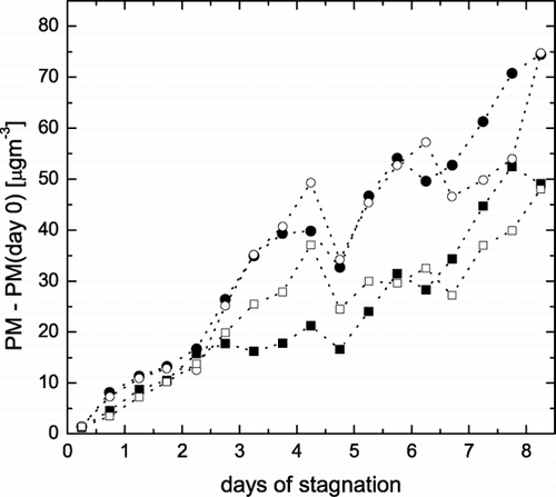
In analyzing the increase in PM concentration during stagnation events, we have selected the periods by three simple criteria: the daily mean concentration in PM₁₀ increases by more than 2 μ g/m³ on each of at least two consecutive days, the initial concentration of PM₁₀ is lower than 30 μ g/m³, and the mean hourly windspeed stays below 1.2 m/s. Figure 7 shows the increase in PM concentration for two of these stagnation events, one in January and one in early March. During the first two days of these stagnation events, the concentration increase in PM₁₀ is almost completely due to the increase in PM₁, whereas at later times the PM₁₀ increases faster than the PM₁ leading to a clear separation of the PM₁ and PM₁₀ data in Figure 7. In the March event a steady state concentration of PM₁ is reached and is by about 20 μ g/m³ higher than at the beginning of the stagnation event. Figure 7c shows the ratio of PM₁ to PM₁₀ for the March event (plotted in Fig. 7a). This general pattern becomes more pronounced when we average over all four stagnation events during which data were collected, as shown in Figure 8: the increase during the first 2½ days is almost entirely accounted for by PM₁ alone, but the later increase is substantially higher for PM₁₀ than PM₁. There is no indication that a steady state is reached in either size class; however the change in slope for PM₁ after ca. 2½ days indicates that these high concentrations and long periods, coagulation might become an important loss mechanism for PM₁ and a corresponding gain mechanism for the PM₁₀. For a rough, order of magnitude estimate, we may take the coagulation coefficient k for the coagulation of two particles with 0.5 μ m diameter as 10^{− 9}cm³·s^{− 1}, and assume the concentration of particles n ₀ being 20,000 cm^{− 3} and that 10 coagulation events are needed to shift a particle from PM₁ to PM₁₀. Then the time t necessary for halving the number concentration will be given by t = 10/(k·n ₀) = 5·10⁵ s which is less than 6 days. This time estimate corresponds well with the measured ratio change with time of Figure 7(c). There are no significant differences in growth behavior of either class at the different sites considered, showing again that the increase is mostly due to secondary material that occurs regionally and not only close to the emission source.

FIG. 7 Increase in PM concentration during stagnation events. (a) Period from the morning of March 11 to the morning of March 18. (b) Period from the evening of January 21 to the morning of January 30. Filled circles: corrected PM₁₀ concentrations; open circles: corresponding PM₁ concentrations. Panel (c) shows the ratio of the PM₁ to PM₁₀ concentrations during the March event (panel (a)).

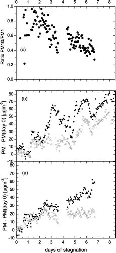
FIG. 8 Twelve hour averaged increase of PM during four stagnation events in 2005/2006. Filled circles:Hönggerberg corrected PM₁₀ concentrations measured with the inlet sharing instrument. Filled squares: corresponding PM₁ concentrations. Open circles: PM₁₀ concentrations over the same time periods at Härkingen. Open squares: corresponding PM₁ concentrations at Härkingen. Linear regression for the entire time period of 8½ days yields the following growth rates: PM₁₀ (our site) = (8.7 ± 0.2) μ g· m^{− 3}· day^{− 1}, PM₁₀ (Härkingen) = (8.3 ± 0.4) μ g· m^{− 3}· day^{− 1}, PM₁ (our site) = (5.5 ± 0.2) μ g· m^{− 3}· day^{− 1}, and PM₁ (Härkingen) = (5.5 ± 0.3) μ g· m^{− 3}· day^{− 1}.

CONCLUSIONS AND OUTLOOK

This work demonstrates that the inlet-time-sharing concept of Ayers (2004) is indeed operationally feasible and advantageous. The instrument behaves as two separate TEOM instruments with different inlets would, as long as hourly (or longer) time averages are considered. It allows—in a very cost effective way—to measure mass concentrations of different size classes and to determine their diurnal and seasonal variation, which can help in characterizing sources and aging of the pollutant particulate matter.

It now appears even possible to further improve the present instrumentation for characterizing PM by taking advantage of a concept described first by Patashnick et al. (2001): one could remove the aerosol particles from the sample stream during short periods by adding an electrostatic precipitator in front of the TEOM mass sensor which is switched on for brief periods after each measurement of the two inlets. Volatilization of previously collected particles on the filter of the TEOM are however continuing, resulting in a frequency increase during these periods, which allows to estimate the mass of the semivolatile fraction under the assumption that the aerosol load in the sampled air do not change during the period and thus to correct the previous mass measurement. The result of a recent field evaluation (Jaques et al. 2004) of this concept with a single inlet yielded very promising results, warranting a field trial of an instrument with time sharing inlets and an electrostatic precipitator.

Acknowledgments

We are grateful to Uwe Weers for technical advice. We thank the EMPA team for providing us with the data of the National Air Pollution Monitoring Network (NABEL). Also, we would like to thank an anonymous reviewer for very helpful comments and for providing an alternative explanation of the diurnal pattern of PM₁.

REFERENCES

- Ayers , G. P. 2001 . Comment on Regression Analysis of Air Quality Data . Atmos. Env. , 35 : 2423 – 2425 .
- Ayers , G. P. 2004 . Potential for Simultaneous Measurement of PM10, PM2.5 and PM1 for Air Quality Monitoring Purposes Using a Single TEOM . Atmos. Env. , 38 : 3453 – 3458 .
- Bohonak , A. J. and van der Linde , K. 2004 . RMA: Software for Reduced Major Axis Regression, Java Version http://www.kimvdlinde.com/professional/rma.htmlWebsite
- Charron , A. , Harrison , R. M. , Moorcroft , S. and Booker , J. 2004 . Quantitative Interpretation of Divergence Between PM10 and PM2.5 Mass Measurement by TEOM and Gravimetric (Partisol) Instruments . Atmos. Env. , 38 : 415 – 423 .
- Chung , A. , Chang , D. P. Y. , Kleeman , M. J. , Perry , K. D. , Cahill , T. A. , Dutcher , D. , McDougall , E. M. and Stroud , K. 2001 . Comparison of Real-Time Instruments to Monitor Airborne Particulate Matter . J. Air Waste Manage. Assoc. , 51 : 109 – 120 .
- Cyrys , J. , Dietrich , G. , Kreyling , W. , Tuch , T. and Heinrich , J. 2001 . PM2.5 Measurements in Ambient Aerosol: Comparison Between Harvard Impactor (HI) and the Tapered Element Oscillating Microbalance (TEOM) System . Science Total Environ. , 278 : 191 – 197 .
- Fisseha , R. , Dommen , J. , Gutzwiller , L. , Weingartner , E. , Gysel , M. , Emmenegger , C. , Kalberer , M. and Baltensperger , U. 2006 . Seasonal and Diurnal Characteristics of Water Soluble Inorganic Compounds in the Gas and Aerosol Phase in the Zurich Area . Atmos. Chem. Phys. , 6 : 1895 – 1904 .
- Gehrig , R. , Hueglin , C. , Schwarzenbach , B. , Seitz , T. and Buchmann , B. 2005 . A New Method to Link PM10 Concentrations from Automatic Monitors to the Manual Gravimetric Reference Method According to EN12341 . Atmos. Env. , 39 : 2213 – 2223 .
- Gomišček , B. , Hauck , H. , Stopper , S. and Preining , O. 2004 . Spatial and Temporal Variations of PM1, PM2.5, PM10 and Particle Number Concentration During the AUPHEP—Project . Atmos. Env. , 38 : 3917 – 3934 .
- Herner , J. D. , Ying , Q. , Aw , J. , Gao , O. , Chang , D. P. Y. and Kleeman , M. J. 2006 . Dominant Mechanisms that Shape the Airborne Particle Size and Composition Distribution in Central California . Aerosol Sci. Technol. , 40 : 827 – 844 .
- Jaques , P. A. , Ambs , J. L. , Grant , W. L. and Sioutas , C. 2004 . Field Evaluation of the Differential TEOM Monitor for Continuous PM2.5 Mass Concentrations . Aerosol Sci. Technol. , 38 : 49 – 59 .
- Patashnik , H. US Patent 3,926,271 . 1975 .
- Patashnick , H. and Rupprecht , E. G. 1979 . A New Real Time Aerosol Mass Monitoring Instrument: The TEOM in Proceedings: Advances in Particulate Sampling and Measurement (Daytona Beach, FL) , Edited by: Smith , W. Washington, D.C. : U.S. Environmental Protection Agency . EPA/600/9-80/004
- Patashnick , H. and Rupprecht , E. G. 1991 . Continuous PM-10 Measurements Using the Tapered Element Oscillating Microbalance . J. Air Waste Manage. Assoc. , 41 : 1079 – 1083 .
- Patashnick , H. , Rupprecht , E. G. , Ambs , J. L. and Meyer , M. B. 2001 . Development of a Reference Standard for Particulate Matter Mass in Ambient Air . Aerosol Sci. Technol. , 34 : 42 – 45 .
- Schwab , J. J. , Spicer , J. , Demerjian , K. L. , Ambs , J. L. and Felton , H. D. 2004 . Long-Term Field Characterization of Tapered Element Oscillating Microbalance and Modified Tapered Element Oscillating Microbalance Samplers in Urban and Rural New York State Locations . J. Air Waste Manage. Assoc. , 54 : 1264 – 1280 .