Asymmetrical Aerosol Deposition in an Idealized Mouth with a DPI Mouthpiece Inlet

Abstract

Monodisperse aerosol deposition in an idealized mouth geometry with a dry powder inhaler (DPI) mouthpiece inlet is studied numerically using a standard Large Eddy Simulation (LES). A steady inhalation flow rate of Q = 90 L/min is used. Ten thousand of particles (4.1 μ m diameter and 953.0 kg/m³ density) are released individually in the computational domain and aerosol deposition is determined. Total aerosol deposition results for the present idealized mouth are in good agreement when compared with measured data obtained in separate experiments, showing improvement over the standard Reynolds Averaged Navier-Stokes/Eddy Interaction Model (RANS/EIM) approach (without near-wall corrections).

INTRODUCTION

Turbulent multiphase flows play an important role in the chemical, pharmaceutical, food, and petroleum industries. Aerosol drug delivery into the lungs through the oral cavity has become an established method in the treatment of lung diseases and has great potential for other non-lung diseases (Finlay 2001). The drug is normally generated in the form of solid or liquid particles from devices such as nebulizers, pressurized metered dose inhalers, pMDIs or “puffers,” and Dry Powder Inhalers, DPIs. Similarly to nebulizers and pMDIs, DPIs (see Borgström 2001) have complex outlet flows (including swirling flows, grid turbulence, jets, and impinging jets), which undesirably will increase particle deposition in the mouth cavity. This outlet complexity comes from the need for DPIs to deagglomerate and disperse medication, since dry powder particles tend to adhere to each other and any surrounding surfaces. On the other hand, DPIs have the advantage of depending only on the inhalation effort of the patient, as opposed to the commonly used pMDIs, which require actuation–inhalation coordination. Although the final target is the lung, part of the dose is usually lost due to deposition in the mouth cavity.

Some insight into undesired mouth deposition can be made using numerical simulation and aerosol deposition experiments. In aerosol deposition simulations involving complex geometries, it is common practice to use Reynolds Averaged Navier-Stokes (RANS) equations combined with standard turbulence models such as k − ϵ, k − ω, or Shear Stress Transport (SST) turbulence models to solve the primary flow and Lagrangian random-walk eddy interaction models (EIMs) to track individual particles in the computational domain. Since RANS simulations give the mean values of flow velocity, turbulence kinetic energy and dissipation, EIMs provide, through modeling, the instantaneous flow velocity values at the particle location. See also Elgobashi (1994) for more details concerning Lagrangian particle tracking simulation techniques.

Previous simulations using standard RANS with Lagrangian random-walk eddy-interaction models (EIM) to track individual particles in the computational domain have shown poor agreement with experimental data on deposition in an idealized mouth–throat region Stapleton et al. (2000). The poor agreement is mainly caused by the fact that particle deposition is dominated by the fluctuation component normal to the wall, which is much smaller than the streamwise and the spanwise fluctuation components in the near-wall region, but assumption of isotropy is normally used in the standard RANS/EIM, causing over prediction of deposition for relatively small particles. More recently, a near-wall correction in the EIM was proposed, yielding significant improvement over previous results, but still falling short from the desired accuracy (Matida et al. 2004a, 2003). Overall, the RANS/EIM results may indicate that the model is not capturing relevant features of the flow, especially near the wall. Other recent numerical investigations using RANS/EIM include studies of aerosol deposition in extrathoracic airways (Xi and Longest 2007; Sosnowski et al. 2006), lung bifurcations (Longest and Vinchurkar 2007), near-wall corrections (Tian and Ahmadi 2007), and investigations of the effect of design on the performance of a Dry Powder Inhaler (Coates et al. 2004).

Considering that particle trajectories can be calculated without eddy interaction modeling as in the RANS/EIM approach, Large Eddy Simulation (LES) is adopted in the present study of deposition of particles in an idealized mouth geometry with a DPI mouthpiece inlet, which generates a swirling flow. Simulated particle deposition results are compared with experimental data obtained in separate work (Matida et al. 2004b). Although much more computationally expensive, LES is known to be more accurate than standard RANS in the simulation of single-phase swirling flows (Pierce and Moin 1998, for LES and Guo et al. 2001, for RANS). In addition, LES has been used to simulate accurately the monodisperse aerosol deposition in channel flows (Wang et al. 1997), pipe flows (Uijttewaal and Oliemans 1996), and 90° bend flows (Breuer et al. 2006b). Prediction of aerosol deposition using LES in an idealized mouth with a small circular inlet (3.18 mm inlet diameter, Matida et al. 2006) was significantly improved over the standard RANS/EIM approach (without near-wall corrections). Although the present approach is applied to aerosol drug delivery, it could be extended to other industrial applications involving one-way coupled aerosol deposition (in which particles do not affect the fluid motion), which is justifiable when the particle concentration in the fluid is low.

Idealized Geometry and Meshing

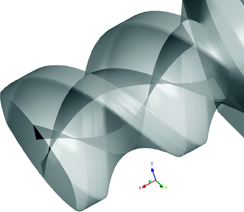
In the present work, an idealized mouth geometry having a commercial DPI (Turbuhaler®, AstraZeneca, Inc.) mouthpiece is used. The DPI mouthpiece consists of a double-helical structure (two internal guide walls) rotating 300 degrees over 13.5 mm of length, which generates a turbulent swirling flow, see Figure 1. The guide vanes are disposed in concurrent planes along the interior of the device as seen in Figure 1.

FIG. 1 Details of the mouthpiece inlet with external walls and internal guide vanes. The twisting angle and the twisting length of the guide vanes cause the highly swirling flow at the outlet of the DPI devise. The design of the mouthpiece geometry not only generates the swirling flow at the outlet but also high vorticity of the flow inside of the device.

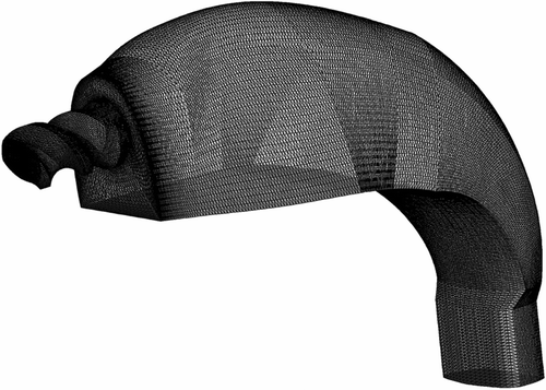
The present idealized geometry is identical to the experimental configuration of the separate aerosol deposition measurements (Matida et al. 2004b). This geometry is an average model for adults based on information available in the literature, supplemented with separate measurements using computer tomography (CT) scans of patients (n = 10) with no visible airway abnormalities and by the observation of living subjects (n = 5). An IGES Initial Graphics Exchange Specification (IGES) mouth geometry file is imported and an unstructured grid having 120 blocks is created using ICEM CFD 5.1 (Ansys, Inc.). The unstructured grid contains approximately 6,000,000 tetrahedral elements (see Figure 2), with biased accumulation of nodes towards the wall and the core of the domain following the mouthpiece inlet jet. Grid convergence analysis for aerosol deposition using the same mouth geometry but different inlet mouthpiece (Matida et al. 2006) has indicated the grid resolution to be adequate. A value of Courant–Friedrich-Levy (CFL) number smaller than unity throughout the computational domain assures the time advancement stability and accuracy, requiring a time step of 1.0 μ s.

FIG. 2 View of grid mesh at the surface of the 3D geometry.

Single-Phase Flow

LES Initial Conditions using a RANS Simulation

The time averaged governing equations of fluid motion (RANS) are solved numerically for the idealized mouth geometry using CFX-10.0 (ANSYS Inc.) software. The Shear Stress Transport (SST) turbulence model along with a second order discretization scheme is used. SST turbulence model is a blending between a k-ϵ turbulence model, which is less sensitive to inlet conditions (when compared against the k-ω turbulence model), and a k-ω turbulence model, which performs well in the near wall region. A steady flow rate of 90 L/min (same as in the experiments by Matida et al. 2004b), turbulence intensity of 10% of the mean velocity and a turbulence length scale of 10% of the inlet diameter defines the inlet conditions. A zero gauge pressure condition was applied at the outlet. A random fluctuation velocity distribution (having an RMS of 5% of the inlet velocity) is added onto the RANS velocity field and is used in the initialization of the LES. In addition to the LES initialization, it is interesting to compare the RANS simulation to the presumably more accurate LES results.

Large Eddy Simulation (LES)

The fluid field is solved using the filtered Navier–Stokes equations along with a standard subgrid scale model and van-Driest wall damping, using CFX-10.0 (ANSYS Inc.) software. Large Eddy Simulation is a result of a space averaging operation applied to Navier–Stokes equations. The filtered Navier–Stokes equations are:

where τ _ij is the subgrid scale (SGS) stress tensor given by

and is modeled. In the present work the SGS stress tensor model proposed by Smagorinsky and Lilly is used. The SGS stresses are related to the strain rate tensor by SGS viscosity, ν _T :

The SGS viscosity ν _T is given by:

where C _s is the Smagorinsky constant (C _s = 0.1 in the present work), D _wall represents the van-Driest wall damping factor, Δ is the filter width and || represents the magnitude of the large-scale strain-rate tensor.

The use of the Smagorinsky model with van-Driest wall damping has proved to be efficient in the simulation of particle deposition on the internal walls of vertical pipe flows (Uijttewaal and Oliemans 1996). More complex SGS stress tensor models have appeared in the literature (for example, the dynamic SGS eddy viscosity models by Germano et al. 1991), but they are beyond the scope of the present work.

A converged RANS velocity field is used to initialize the LES simulation. A central difference advection scheme is used, while for the time marching a second order accurate backward Euler formula is used. A transient start-up period of 25,000 time steps is used to ensure that the effect of the initial conditions has decayed. An additional 8,000 time steps is used in the particle deposition simulation. Calculations were performed on a Pentium IV cluster having 20 nodes, requiring 328 CPU hours.

RANS/Eddy Interaction Model

When the RANS equations are used, the instantaneous quantities are composed of a mean part and a fluctuating component

where U _i +u′ _i will substitute u _i in Equation (7).

When using the mean flow velocities obtained from RANS simulation, the local fluctuating velocities must be obtained through modeling (EIMs, eddy interaction models or random walk models). In the present work, RANS particle simulations without modeling (artificially assuming fluid flow fluctuation velocities to be zero) will be denoted as “mean flow tracking” and particle simulations with EIM modeling will be referred to as “turbulent tracking.”

In EIMs, one particle is allowed to interact successively with various eddies. Each eddy has a characteristic lifetime, length, and velocity scales. The end of interaction between the particle and one eddy occurs when the lifetime of the eddy is over or when the particle crosses the eddy. At this instant, a new interaction with the particle and a new eddy is started. For the simple EIMs used here, the local fluctuating velocities are obtained by multiplying the root-mean square (RMS) fluid fluctuating velocity

by random numbers (N _u , N _v , N _w ) generated from a Gaussian probability density function of zero mean and unity standard deviation at the start of eddy-particle interaction. The length, time, and velocity scale of fluid eddies can be obtained from:

where C _μ = 0.09, k is the turbulence kinetic energy and ϵ is the dissipation.

Particulate Phase

Particle Equation of Motion

The particle-laden flow is predicted by an Eulerian-Lagrangian approach. The continuous phase is determined by LES in the Eulerian frame of reference whereas the dispersed phase is determined in the Lagrangian frame of reference by simultaneously tracking a large number of individual particles through the continuous flow field. A large number of particles (10,000) with a diameter of 4.1 μ m and density of 953 kg/m³ are released in the calculated flow domain and particle depositions are recorded. Simulations with 20,000 particles show 10,000 particles to be adequate when particle deposition is concerned, since deposition differed by less than 1.1% between the two cases. The volume fraction of the particles is small (V _fraction = 8.744 × 10⁻⁷) and hence only one-way coupling is taken into account. The particles are assumed to be rigid and spherical and no Brownian motion of the particles is taken into account since the size of the particles is large enough to neglect its effect.

For the case of small particles (2.5–5 μ m) with low density ratios ρ _f /ρ _p ≪ 1 and taking into account only viscous drag and gravity, the three-dimensional Lagrangian equation that describes the motion of particles in Cartesian coordinate system is given by

where v _i corresponds to the particle velocity components, u _i to the instantaneous fluid flow components at the particle location, g _i to the gravitational components, and α is a drag correction factor that extends the validity of the Stokes flow regime for higher particle Reynolds numbers (Schiller and Naumann 1933). For the case of LES, u _i corresponds to ū _i or the filtered velocity components. The term

represents the effect of the drag force exerted on the particle. The particle relaxation time is given by

and

In Equation (10), Re _p represents the particle Reynolds number. The drag force on the particle is based on Stokes flow around a sphere, i.e., C _D = α 24/Re _p where α is a correction factor used to extend the validity of the relation for high particle Reynolds number (0 < Re _p < 800). Integrating Newton's second law leads to the particle velocity. Using the definition of the particle velocity, the actual position of the particle can be determined by a second integration.

Particles are released in a “frozen” computational domain at a given time step (after 25,000 initial time steps, to ensure that the initialization effects are vanished). “Frozen-domain” in this manuscript represents a snapshot of the 3-D fluid flow containing the instantaneous values of the velocity field at a particular time step. Breuer et al. (2006a) recently performed particle tracking simulations in an idealized mouth with a small inlet, using both “frozen-domain” and dynamic LES (where different groups of particles are released at different time steps and tracked over time). They found that the “frozen-domain” and “dynamic” particle tracking approaches gave similar results and both were in good agreement when compared with experimental data. Although dynamic particle tracking could also be used, it would be prohibitively expensive computationally in the present simulation and the “frozen-domain” particle tracking is adopted. Initial particle velocities are set equal to the fluid velocity.

RESULTS AND DISCUSSION

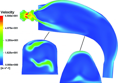
Figure 3 shows the magnitude of mean velocities from the RANS simulation at the midplane of the idealized mouth at a steady inhalation flow rate, Q = 90 L/min. In addition, the velocities at two cross-sections are also shown in the figure.

FIG. 3 Magnitude of mean velocities (0–65 m/s range, RANS simulation).

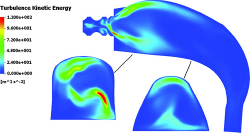
Similar plots for turbulence kinetic energy, k, are shown in Figure 4.

FIG. 4 Turbulence kinetic energy (0–120 m²/s² range, RANS simulation).

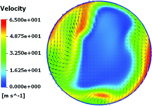
Figure 5 shows the magnitude of mean velocities superimposed by a 2-D vector plot (velocity vectors at the cross sectional plane without the streamwise component) at the exit of the mouthpiece (or inlet of the mouth cavity).

FIG. 5 Magnitude of mean velocities and 2-D velocity plot at the exit of mouthpiece (from RANS simulation).

Figure 6 shows the magnitude of instantaneous velocity from LES after 25,000 time steps superimposed by a 2-D vector plot at the exit of the mouthpiece.

FIG. 6 Magnitude of instantaneous velocities and 2-D velocity plot at the exit of mouthpiece (from LES simulation).

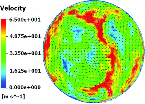
From Figure 5 and Figure 6, it can be seen that LES captures small fluid eddy structures (determined by grid size) and provides a better description of the fluid flow behavior than RANS. Examining Figure 5 and Figure 6, although near the wall region both RANS and LES seem to predict similar swirling tendencies of the flow, in the core of the domain, RANS differs considerably from the LES flow field. The high values of velocity magnitude in the core of the domain in Figure 6 are due to the two helically guiding vanes, which generate the swirling flow at the exit of mouthpiece.

Figure 7 shows the magnitude of instantaneous velocity from LES after 25,000 time steps at the same midplane as in Figure 3.

FIG. 7 LES instantaneous magnitude of velocities after 25,000 time steps.

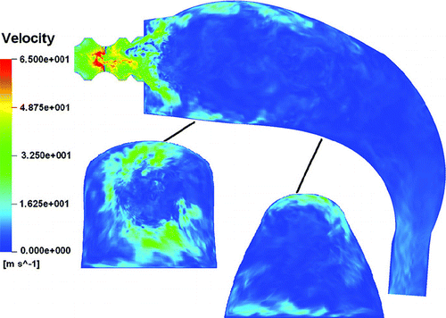
The supremacy of LES over RANS can be seen by comparing Figure 7 and Figure 3, with LES providing more complete information (eddy and vortical structures) about flow field behavior. After the mouthpiece, the swirling flow spreads rapidly towards the wall of the mouth. Note that the inlet swirling flow has a non-symmetrical preferential path on one side of the mouth with localized and partial impingement of the inlet swirling jet on the anterior part of the mouth with relatively high levels of turbulence kinetic energy distribution. It is clearly shown from Figure 5 and Figure 6 that the swirling flow is already non-symmetrical at this location, anterior to the idealized mouth.

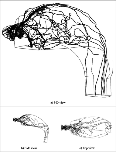
For particle deposition, ten thousand particles having a diameter of 4.1 μ m are released in the “frozen” LES computational domain as described in the previous section and aerosol deposition results are recorded. An example of particle trajectories is depicted in Figure 8 for 50 particles (4.1 μ m) released randomly at the inlet of the mouthpiece and followed until they deposit on the walls or leave the computational domain at the outlet. Particles are seen to be preferentially thrown to the sides of the oral cavity upon entry, with their resulting proximity to the walls resulting in significant deposition. The total deposition of particles is obtained from the ratio of the number of particles that deposited on the walls to the total number of particles that were released in the computational domain from the inlet.

FIG. 8 Visualization of 50 trajectories of 4.1 μ m diameter particles in the mouth cavity with a DPI mouthpiece inlet; LES simulation.

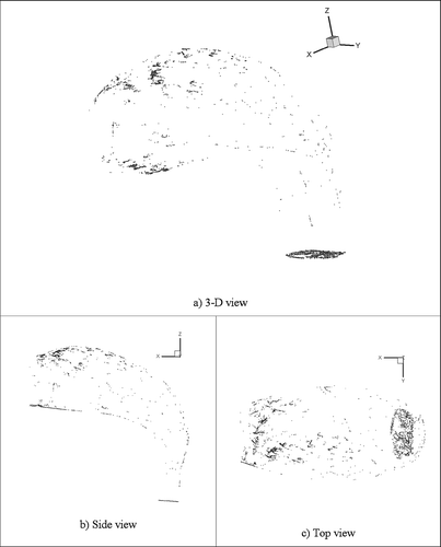
Figure 9 shows the particle deposition distribution on the surface and the outlet of the idealized geometry for 10,000 released particles. Simulated deposition patterns show non-uniform deposition characteristics (particles deposited more on the anterior part of the mouth, particularly on the patient's left side) due to the non-symmetric swirling flow coming out of the DPI mouthpiece. The numerical simulation results show that 43.3% of the total particles deposit on the right side while 56.7% of the particles deposit on the left side.

FIG. 9 Particle deposition distribution (at the surface of geometry) from LES.

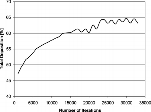
Figure 10 shows the total deposition as a function of the number of iterations (i.e., time steps). It can be seen that the total deposition (T.D.) of particles oscillates around an asymptotic average value (T.D. = 63%) after 25,000 time steps.

FIG. 10 Total aerosol deposition using LES.

It is shown in Figure 11 that this average total deposition using LES (T.D. = 63%) agrees well with the experimental value (T.D. = 67%, Matida et al. 2004b), for particles with a diameter of 4.1 μ m, whereas the RANS/EIM “turbulent tracking” (T.D. = 76%) shows over-prediction and the RANS/EIM “mean flow tracking” (T.D. = 43%) shows a considerable under-prediction. The “mean flow tracking” represents aerosol deposition by inertial impaction, and “turbulent tracking” adds aerosol deposition by modeled turbulent dispersion. The percentage errors against the experimental value of deposition are calculated for each approach (“turbulent tracking,” LES, and “mean flow tracking”) and shown in Table 1.

FIG. 11 Numerical and experimental (Matida et al. 2004b) results of total particle deposition for a particle size (d _p = 4.1 μ m). “Turbulent Tracking” and “Mean Flow Tracking” are from RANS/EIM simulations.

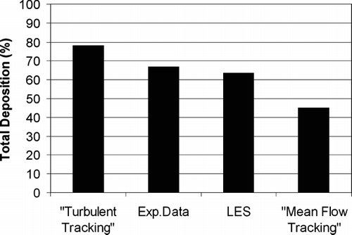
TABLE 1 Percentage error in Total Deposition for each numerical approach compared to experimental values

Numerical approach	RANS Mean Flow Tracking	RANS Turbulent Tracking	LES
Total Deposition (%)	43	76	63
Percentage error (%)	35.82	13.43	5.97

The percentage errors against the experimental value of deposition are calculated for each approach (“turbulent tracking,” LES, and “mean flow tracking”) and shown in Table 1.

CONCLUSION

The present work shows that a standard LES (Smagorinsky/Lilly subgrid scale model with a van-Driest wall damping function) with particle tracking in a “frozen” flow can be used in the prediction of the deposition of particles in an idealized mouth with a DPI mouthpiece inlet for a particle size of 4.1 μ m, relevant to pharmaceutical aerosols, and an inhalation flow rate of 90 L/min. The deposition pattern in the mouth proved to be asymmetrical for this particular DPI inhaler for the present fluid flow and particle size conditions. LES seems to capture relevant features of the flow that standard RANS/EIM does not reproduce, mainly in the wake of the mouthpiece inlet jet and in the near-wall region. Total deposition simulation results with LES show good agreement when compared with measured data obtained in separate experiments (Matida et al. 2004b), giving an improvement over the standard RANS/EIM approach, but increasing computational requirements significantly. It is conjectured here that the small discrepancies between the LES and the experiments might be reduced by the introduction of higher grid resolutions; dynamic particle tracking (where effects on aerosol deposition by turbulent structures with larger length or time scales could be a factor) and/or alternative SGS stress tensor modeling. It should be emphasized that a LES using the same geometry and grid size, but having a realistic inhalation cycle (not a steady flow rate at the inlet as in the present simulation) would require an impractical computational time for the computational resources available in the present work, stressing the need for further developments regarding the RANS/EIM approach (probably using near-wall corrections).

REFERENCES

- Borgström , L. 2001 . On the Use of Dry Powder Inhalers in Situations Perceived as Constrained . J. Aerosol Med. , 14 ( 3 ) : 281 – 287 .
- Breuer , M. , Durmus , G. , Matida , E. A. and Finlay , W. H. LES and an Efficient Lagrangian Tracking Method for Predicting Aerosol Deposition in Turbulent Flows . Fifth Int. Symposium on Turbulence, Heat and Mass Transfer (THMT-5) . Dubrovnik, Croatia.
- Breuer , M. , Baytekin , H. T. and Matida , E. A. 2006b . Prediction of Aerosol Deposition in Bends Using LES and an Efficient Tracking Method . J. Aerosol Sci. , 37 ( 11 ) : 1407 – 1428 .
- Coates , M. S. , Fletcher , D. F. , Chan , H.-K. and Raper , J. A. 2004 . Effect of Design on the Performance of a Dry Powder Inhaler Using Computational Fluid Dynamics. Part 1: Grid Structure and Mouthpiece Length . J. Pharma. Sci. , 93 ( 11 ) : 2863 – 2876 .
- Elgobashi , S. 1994 . On Predicting Particle-Laden Turbulent Flows . Appl. Sci. Res. , 52 : 309 – 329 .
- Finlay , W. H. 2001 . The Mechanics of Inhaled Pharmaceutical Aerosols: An Introduction , London : Academic Press .
- Germano , M. , Piomelli , U. , Moin , P. and Cabot , W. H. 1991 . A Dynamic Subgrid-Scale Eddy Viscosity Model . Physics of Fluids A , 3 ( 7 ) : 1760 – 1765 .
- Guo , B. , Lnangrish , T. and Fletcher , D. 2001 . Simulation of Turbulent Swirl Flow in an Axisymmetric Sudden Expansion . AIAA J. , 41 ( 1 ) : 96 – 102 .
- Longest , P. W. and Vinchurkar , S. 2007 . Effects of Mesh Style and Grid Convergence on Particle Deposition in Bifurcating Airway Models with Comparisons to Experimental Data . Medical Engineering and Physics , 29 ( 3 ) : 350 – 366 .
- Matida , E. A. , Finlay , W. H. , Breuer , M. and Lange , C. F. 2006 . Improving Prediction of Aerosol Deposition in an Idealized Mouth Using Large Eddy Simulation . J. Aerosol Med. , 19 ( 3 ) : 290 – 300 .
- Matida , E. A. , Finlay , W. H. , Lange , C. F. and Grgic , B. 2004a . Improved Numerical Simulation of Aerosol Deposition in an Idealized Mouth-Throat . J. Aerosol Sci. , 35 : 1 – 19 .
- Matida , E. A. , Rimkus , M. , Grgic , B. , Lange , C. F. and Finlay , W. H. 2004b . A New Add-On Spacer Design Concept for Dry-Powder Inhalers . J. Aerosol Sci. , 35 : 823 – 833 .
- Matida , E. A. , DeHaan , W. H. , Finlay , W. H. and Lange , C. F. 2003 . Simulation of Particle Deposition in an Idealized Mouth with Different Small Diameter Inlets . Aerosol Sci. Technol. , 37 : 924 – 932 .
- Menter , F. R. 1994 . Two-Equation Eddy-Viscosity Turbulence Models for Engineering Applications . AIAA J , 32 ( 8 ) : 1598 – 1605 .
- Pierce , C. D. and Moin , P. 1998 . Method for Generating Equilibrium Swirling in Flow Conditions . AIAA J , 36 ( 7 ) : 1325 – 1327 .
- Stapleton , K. W. , Guentsch , E. , Hoskinson , M. K. and Finlay , W. H. 2000 . On the Suitability of k −ϵ Turbulence Modeling for Aerosol Deposition in the Mouth and Throat: A Comparison with Experiment . J. Aerosol Sci. , 31 ( 6 ) : 739 – 749 .
- Schiller , L. and Naumann , A. 1933 . A Drag Coefficient Correlation . VDI Zeitschrift , 77 : 318 – 320 .
- Sosnowski , T. R. , Moskal , A. and Grandon , L. 2006 . Dynamics of Oropharyngeal Aerosol Transport and Deposition with the Realistic Flow Pattern . Inhal. Toxicol. , 18 ( 10 ) : 773 – 780 .
- Tian , L. and Ahmadi , G. 2007 . Particle Deposition in Turbulent Duct Flows-Comparisons of Different Model Predictions . Aerosol Sci. , 38 : 377 – 397 .
- Uijttewaal , W. S. J. and Oliemans , R. V. A. 1996 . Particle Dispersion and Deposition in Direct Numerical and Large Eddy Simulations of Vertical Flows . Physics of Fluids , 8 ( 10 ) : 2590 – 2604 .
- Wang , Q. , Squires , K. D. , Chen , M. and McLaughlin , J. B. 1997 . On the Role of the Lift Force in Turbulence Simulations of Particle Deposition . Intl. J. Multiphase Flow , 23 ( 4 ) : 749 – 763 .
- Xi , J. and Longest , P. W. 2007 . Transport and Deposition of Micro-Aerosols in Realistic and Simplified Models of the Oral Airway . Annals of Biomedical Engineering , 35 ( 4 ) : 560 – 581 .