Airborne Phase Doppler Interferometry for Cloud Microphysical Measurements

Abstract

Conducting accurate cloud microphysical measurements from airborne platforms poses a number of challenges. The technique of phase Doppler interferometry (PDI) confers numerous advantages relative to traditional light-scattering techniques for measurement of the cloud drop size distribution, and, in addition, yields drop velocity information. Here, we describe PDI for the purposes of aiding atmospheric scientists in understanding the technique fundamentals, advantages, and limitations in measuring cloud microphysical properties. The performance of the Artium Flight PDI, an instrument specifically designed for airborne cloud measurements, is studied. Drop size distributions, liquid water content, and velocity distributions are compared with those measured by other airborne instruments.

NOMENCLATURE

A	=	amplitude of the Doppler burst signal
ρ d	=	droplet density
u d	=	droplet incoming velocity
ν	=	fluid kinematic viscosity
ƒ r	=	fluid oscillation frequency
u ƒ	=	fluid velocity
η	=	Kolmogorov length scale
σ n	=	measurement noise (including detector shot noise, etc.)
N	=	number of data points sampled by the instrument within each burst
ƒ s	=	sampling frequency
ϵ	=	turbulent kinetic energy dissipation rate
ρƒ	=	fluid density
τ c	=	noise correlation time scale
d	=	drop diameter
D beam	=	effective diameter of the laser beams (is a function of d)
D transit	=	maximum transit length
F	=	focal length of the front focusing lens
F/PDI	=	flight PDI
ƒ D	=	Doppler frequency
ƒ g	=	characteristic gravitational settling frequency
K 0, K 1	=	fitting constants
l	=	the average spacing between sampled droplets
L aperture	=	length of view volume defined by aperture, and is labeled
l transit	=	transit distance through the view volume
LWC	=	total liquid water content
n	=	cloud drop number density
P	=	probability distribution function
PDI	=	phase Doppler interferometer
PVD	=	probe volume diameter
Q sample	=	volume of air sampled per unit time
s	=	beam separation before reaching the focusing lens
s	=	drop slip velocity
SNR	=	signal to noise ratio
t r	=	transit time
u	=	component of the droplet velocity perpendicular to the fringe plane
U	=	component of flight velocity in the probe axis
u r	=	velocity fluctuation scale associated with spatial scale r
W	=	width of receiver aperture
δ	=	fringe spacing
φ	=	phase shift between Doppler bursts
γ	=	laser beam intersection angle
λ	=	wavelength of the laser
θ	=	photodetector receiver angle
σ	=	instrument measurement cross section
τ d	=	droplet inertial time scale

1. INTRODUCTION

The cloud droplet number size distribution (sometimes termed the cloud droplet spectrum) is the fundamental microphysical description of a cloud. In situ measurement of this distribution via an airborne platform is the only way to study many clouds at the droplet scale, and therefore has been the subject of much research.

Most contemporary optical techniques for measuring cloud droplet size distributions from airborne platforms are based on the determination of droplet size from measurement of scattered light intensity. The standard instrument for measurements of cloud droplet size distributions (in the approximate diameter range of 5 to 50 μ m) over the last 25 years has been the PMS Forward Scattering Spectrometer Probe (FSSP). Briefly, the instrument detects light scattered by droplets when they traverse a focused laser beam. Two detectors with different geometries allow for determination of whether a droplet is within the “depth of field” and near the relatively uniform focal point of the laser beam where droplet diameter can be related to measured intensity (for spherical droplets). Over the years it has been shown that the FSSP can experience significant sizing errors due to droplet coincidence in the laser beam (Cooper 1988), and that droplet sampling can be biased due to variations in the effective size of the sample volume, flow distortions or droplet shattering on the instrument housing (e.g., Gerber et al. 1999; Glantz et al. 2003). Furthermore, nonuniform intensity and inhomogeneities in the beam profile can lead to artificial broadening of the measured size distributions (Wendisch et al. 1996). Several of these problems have been improved upon in subsequent modifications, including the Fast-FSSP, which improves the electronics and minimizes dead-time effects (Brenguier et al. 1998), and the M-Fast FSSP, which makes possible a procedure for minimizing beam-inhomogeneity effects (Schmidt et al. 2004). However, coincidence effects tending to broaden the measured size distribution are still difficult to overcome (de Araujo Coelho et al. 2005).

An example of a recent instrument that operates in the size range of approximately 10–1000 μ m is the 2D-S (Lawson et al. 2006). The instrument measures particle “shadowgraphs” from two crossing laser beams with two linear photodiode arrays. The stereo aspect of the instrument should improve the sample volume determination over previous linear-diode instruments such as the 2D-C that suffered from a particle-size-dependent sample volume for small particles. However, out-of-focus drops are still present in each of the beams and can contribute to the sizing uncertainty. Advantages are the relatively large sample volume and the ability to measure nonspherical particles.

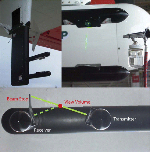
The purpose of this article is to describe a new probe for cloud drop size distribution measurements. The instrument utilizes the well-known technique of phase Doppler interferometry or PDI (Bachalo 1980; Bachalo and Houser 1984), which will be described briefly below. PDI is a well-established technique in the liquid atomization and spray sciences community, but is much less common in cloud physics. Our goals are to (a) briefly describe the PDI technique in such a way that cloud physicists outside the PDI field can understand the advantages and limitations of the technique and (b) describe the capabilities and performance of a new airborne PDI-based instrument intended to make measurements of the cloud drop size distribution as well as the cloud drop velocity distribution. This new instrument, the Artium Flight-PDI (or F/PDI), was designed and constructed by Artium Technologies, Inc. of Sunnyvale, CA. Figure 1 shows three views of the Artium F/PDI. The same technique can be used to examine issues related to the effects of microscale turbulence on clouds (Saw et al. 2007), such as measuring cloud drop spacing. These issues will be described in detail in a future article and therefore will not be further discussed here.

FIG. 1 Three photos showing the Artium F/PDI. The upper left pannel shows the instrument mounted vertically on board the CIRPAS Twin Otter (mounting can also be horizontal). The upper right panel shows a pre-flight test where a spray paint nozzle produces a distilled water spray at reasonably high velocity (∼ 5 m/s). The crossing laser beams are clearly visible. The beams emerge from the upper arm, and are stopped by a beam stop on the lower arm. The scattered light enters the lower arm and is sensed by three photodetectors. The lower panet shows a front-on view of the two arms and the relative location of the view volume. The instrument body is 28 × 56 × 6.6 cm; each arm is 30 cm long and 3 cm in diameter; the arms are 15 cm apart. (Figure is provided in color online.)

2. PHASE DOPPLER INTERFEROMETRY: PRINCIPLES AND PERFORMANCE

The PDI technique ¹ has been previously described in great detail in the literature (e.g., Bachalo 1980; Bachalo and Houser 1984; Bachalo and Sankar 1996; Davis and Schweiger 2002). Here, we outline the fundamental operating principles in order to aid potential instrument and data users, and other interested parties, in understanding the technique. The measurement principle is based on light scattering interferometry, which utilizes the wavelength of light as the measurement scale. In contrast, almost all existing optical probes utilize the intensity of scattered light to make the measurement. This confers PDI with certain advantages, primarily independence on any light beam attenuation or changes in light intensity with significantly improved performance under conditions of contaminated optics and/or electronic drift and noise, and a significantly reduced need for calibration.

The optical system for PDI is similar to that of laser Doppler velocimetry, and is shown schematically in Figure 2. The measurement volume is established by the intersection of two focused and identical beams (derived from a single polarized laser) intersecting at a known angle. In this intersection volume, the cross section of intensity has two components: (1) a low-frequency Gaussian profile that results from the Gaussian profile of each of the individual identical beams; and (2) a high frequency sinusoidal pattern that results from constructive and destructive interference of these two beams (Figure 2). The exact fringe pattern depends on the laser wavelength and the beam intersection angle. The inter-fringe spacing, δ, is determined for small intersection angles by the wavelength of the laser λ, and the beam intersection angle γ according to (Bachalo and Houser 1984):

For small γ, the equation can be simplified as shown to be a function of the focal length F of the front focusing lens, and the beam separation before reaching the focusing lens, s. The view volume of the instrument is defined by the portion of the laser intersection volume that is imaged through the aperture by the detectors, and looks approximately like a cylinder as shown schematically in Figure 2. The effective length of the view volume is the dimension defined by the aperture, and is labeled L _aperture (see Section 2.3 for more detail). The view volume diameter is defined by the diameter of the laser beams D _beam (Figure 2). Precise determination of the view volume is described in detail below.

FIG. 2 Schematic of a PDI instrument. Laser is split by the beam splitter into two equal-intensity beams. The two beams are brought together at angle γ using the front focal lens. The measurement volume is the intersection of the two beams (where each beam is also focused), which for small γ is approximately a cylinder with dimensions D _beam and L _aperture. The scattered light is collected, spatially filtered using an aperture, and then imaged onto a set of three detectors labeled A, B, and C. The detector signals are then processed to produce individual drop size and velocity. The receiver is located at an angle θ from the transmitter optics. Note that γ is greatly exaggerated in this schematic.

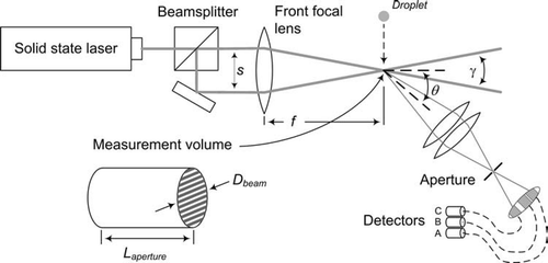
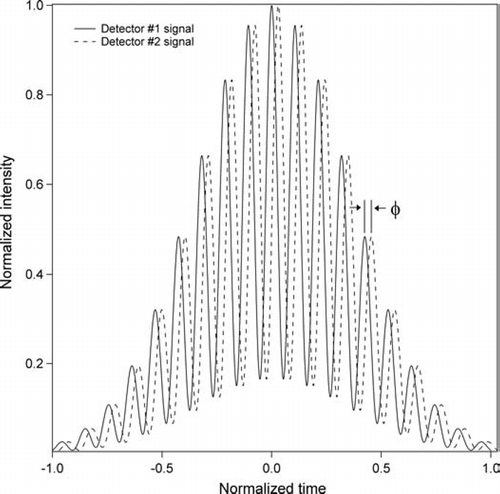
As a droplet passes through the beam intersection volume, it scatters light into the surrounding space. The receiver is situated at a suitable off-axis angle, θ, to collect this scattered light and image it onto a series of detectors; for simplicity we will describe a two detector system (although in practice three detectors are used by the F/PDI to increase the dynamic range for drop sizing and for signal validation). Each detector records a time-varying signal that, like the view volume, exhibits an overall Gaussian intensity profile on which a higher frequency sinusoid is superimposed. These signals, illustrated in Figure 3, are termed “Doppler bursts” and represent the raw data collected, from which all other quantities (primarily drop size and velocity) are derived, as described below. Because the signals produced with this method have a unique sinusoidal character, the use of digital detection techniques can easily discriminate signal from noise even when the signal-to-noise ratio (SNR) is low, an important advantage for proper drop counting in potentially noisy environments such as aircraft. The characteristic signal also permits discrimination of coincident events from single drop events, as well as non-spherical particles from spherical ones, since in both cases the actual signal differs from the expected signal for a single spherical drop.

FIG. 3 Schematic of idealized photodetector signals received by two detectors. Primary characteristics are a Gaussian envelope in intensity, on which a higher frequency sinusoid is superimposed. Frequency of either of the signals yields drop velocity. The phase shift between the two signals φ is a measure of the drop size.

Accurately deriving δ is critical for all subsequent measurements, as uncertainty in the value of δ biases the measurement of velocity and size. From Equation (1), λ and F are quantities that are known to very high accuracy and precision and also are essentially constant under normal operation. Therefore, the uncertainty in δ depends on the ability to properly measure s. Normally, s is measured by directing the transmitter beams onto a distant wall. By measuring the distance to the wall, and the beam separation at this distance, s can be calculated to within < ∼ 1%. The potential exists for reducing this uncertainty in s to ∼ 0.1% using an independent velocity calibration standard.

2.1. Measurement of Drop Velocity

Each Doppler burst will exhibit a Doppler frequency, ƒ _D from which the velocity of the droplet can be derived (Figure 3). The velocity can be related to the fringe spacing by the simple formula:

where u is the component of the droplet velocity in the direction perpendicular to the fringe plane, and ƒ _D is the frequency of the Doppler burst. Frequency can be measured to very high precision, and thus the uncertainty in u is dominated by the uncertainty in δ, which in turn is dictated by the uncertainty in s. If there is an independent measure of the velocity of the instrument relative to the mean flow (as is almost always the case for airborne applications where true airspeed is measured), then s can be checked.

2.2. Measurement of Drop Size

The second property of the two signals is the phase shift φ between them (Figure 3), which has been shown to have a nearly monotonic, linear relationship with droplet diameter (Bachalo and Houser 1984). The origin of this phase shift can be understood by considering the droplet as a small lens that refracts light as it falls through the view volume (illustrated in Figure 4). If one were to freeze the motion of the droplet “lens” as it passes through the measurement region, one would find that the lens projects a magnified image of the interference fringes into surrounding space. The smaller the droplet, the more expanded the projected fringes will be in the surrounding space because the radius of curvature of the lens is smaller. It is this spatial frequency of the projected fringe pattern that is measured by the phase shift between two detectors. The analogy of a particle as a lens suggests two important properties that particles must satisfy in order that PDI be a successful technique: they must be optically homogeneous at a length scale small relative to the size of the drop (paint and other slurry droplets have been measured with this method) with known refractive index, and they must be close to spherical. In the case of liquid cloud droplets, this will be satisfied under most realistic atmospheric conditions for drops in the diameter range of 2 μ m to 1 mm (all drop sizes herein are reported as diameter d).

FIG. 4 Schematic illustrating origin of the phase shift versus diameter relationship. A small drop (top) yields a small phase shift, whereas the larger drop (below) yields a larger phase shift.

In actual PDI applications, three unequally-spaced detectors, such as those labeled A, B, and C in Figure 2, are used. This permits unambiguous measurement over phase differences of up to 3 cycles (3 × 360° = 1080°) because the phase differences between all three detector pair possibilities—φ _AB , φ _AC , and φ _BC can be used. Such redundant measurements allow a greater measurement range of droplet size than would be possible using a single pair of detectors, i.e., only φ _AB , as well as much higher sensitivity. In addition to providing much higher sensitivity, the pairs of detectors provide redundant measurements of each drop providing valuable means for evaluating each measurement.

Under these conditions, the phase difference between the signals is a direct measure of the diameter of the spherical particle, and the two quantities are linearly related as long as a single light scattering mechanism dominates, namely, refraction or reflection (Bachalo and Houser 1984). At very small droplet sizes, diffraction can become significant relative to refraction, and lead to oscillations in the φ versus d relationship at the smallest drop sizes, primarily in the size range below 4 μ m, but with some effects up to ∼ 8 μ m (Bachalo and Sankar 1996). These oscillations affect the droplet size measurement precision in this size range, resulting in a measurement uncertainty of approximately +/– 0.5 μ m (Bachalo and Sankar 1996). The problem can be reduced by using a larger off-axis detection angle when accurate measurements of small droplets (0.5 to 10 μ m) is desired, at the expense of limiting the upper size range of measurable drops. At visible wavelengths, the practical smallest measurable size using PDI is ∼ 0.5 μ m, limited by both sizing ambiguities as well as signal to noise ratio (SNR).

The ultimate limits on PDI at the large size range for natural water drops is determined by drop sphericity. Very large drops deviate from a spherical shape due to aerodynamic drag forces, and therefore can be sized with proportionate uncertainty. If the large drops are oscillating randomly, the mean size will be determined with reasonable uncertainty, while the drop size distribution will be somewhat broadened. Droplets smaller than 300 μ m are generally nearly perfect spheres, and maximum uncertainty of ∼ 2% and ∼ 10% due to asphericity may be expected for drops of 1 mm and 2 mm, respectively (Pruppacher and Klett 1997). There are other issues once drops become very large relative to the sample volume diameter, such as the possibility of reflection becoming significant relative to refraction, although such issues can be dealt with (e.g., Bachalo 1994). It is straightforward to produce large beam diameters to optimize measurement of large drops, with the trade-off of increasing the size of the smallest measurable drop. In practice, the utility of PDI for such large droplets depends on the choice of beam diameter and the resulting sample volume. More advanced dual range instruments (two PDI systems co-located in one measurement volume using two different laser wavelengths) are in development, permitting measurement of drops from 2 to 1500 μ m.

The dynamic size range that F/PDI can cover is governed by limitations on dynamic range of the photodetectors. Presently, a dynamic range of 2500:1 in detected amplitude range by the photodetectors is realistic, and this leads to a dynamic range of ∼ 50:1 in drop diameter. The detector gain can be adjusted in real-time in a less than a second to shift the 50:1 dynamic size range if desired. At the smallest drop sizes, the entire dynamic range may not be achievable in reality if the photodetectors exhibit high noise levels, i.e., if SNR is too low. By using lasers with adequate power and detectors with high sensitivity, it is has been possible to design an instrument capable of reliable operation and reasonable sampling statistics within the diameter range of 3–150 μ m.

PDI requires only a single calibration to accurately establish the optical parameters including the detector separations. Since the components are mechanically and optically rigid and fixed, additional field calibrations are not required. The calibration establishes the φ versus d relationship. This is typically accomplished using a monodisperse drop generator, which generates a steady stream of drops of known size (and very low size variance) by driving a periodic instability at the appropriate frequency into a laminar a liquid jet, leading to break-up of the stream into nearly uniform drops (Schneider and Hendricks 1964). As is typical, the drop generator used to calibrate the Artium F/PDI utilizes a piezo-electric crystal connected to a signal generator to cause drop break-up into a stream with known mean drop size. The liquid stream is forced using a syringe pump. The resulting drop stream is used to size calibrate the F/PDI.

We have conducted tests of the F/PDI sizing capabilities under laboratory conditions using glass beads (Duke Scientific, Inc.), which were specified by the manufacturer to have a diameter of 30.1 ± 2.1 μ m. The F/PDI-derived values were 30.7 ± 3.0 μ m, which agrees in the mean very well with the manufacturer specifications, and exhibits a slight amount of broadening (∼ 1 μ m).

2.3. Measurement of Concentration

To calculate the drop number size distribution, the volume of air sampled per unit time Q _sample must be determined. On a moving platform, Q _sample is determined by three parameters:

D _beam(d) is the effective laser beam diameter as a function of drop diameter d (thus making Q _sample a function of d as well), and is derived from an in situ measurement method to determine the sample volume size as a function of the droplet size under the prevailing measurement conditions. Recall (Section 2 and Figure 2) that the view volume can be approximately represented as a cylinder. L _aperture is the length of the view volume as defined by the receiver aperture whose width W determines L _aperture according to L _aperture = W/m sin θ, where m and θ are the magnification and off-axis angle of the receiver optics. For the F/PDI, apertures of width 0.05, 0.1, 0.2, 0.5, and 1 mm are mounted to a motorized mechanism, allowing the operator to select via software the aperture size most appropriate for the sampling conditions. U is the velocity of the instrument relative to the atmosphere (i.e., true air speed for airborne applications), and is most easily determined from an average of the F/PDI in situ velocity measurements of the sampled drops.

D _beam is a function of d because the laser beam has a Gaussian intensity profile, which implies that the incident light intensity on the drops depends upon their trajectory through the beams. Drops that transit the view volume further from the center of the beams scatter less light (Bachalo and Sankar 1996). Therefore, for a given drop size, there is some D _beam at which minimum SNR is reached. Because larger drops scatter more light (approximately proportional to d ²), they can pass through parts of the beam farther from the center than smaller drops. As a result, larger drops exhibit larger D _beam at constant SNR. This tends to be advantageous for sampling natural clouds, because under most conditions, the concentration of smaller drops is much higher relative to larger drops. Thus, the smaller D _beam for small drops helps reduce coincidence problems, while the larger D _beam for larger drops increases the counting statistics of these rarer events. Over the dynamic size range of the instrument, D _beam for the smallest to largest drops varies by approximately an order of magnitude.

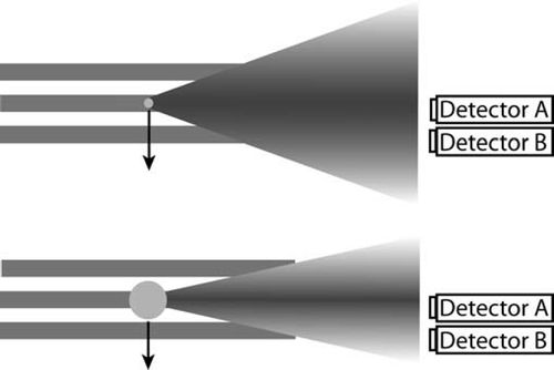
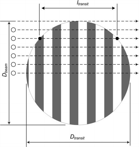
In order to determine D _beam(d), we assume that the probe volume is a cylinder, with the length of the cylinder being L _aperture, and the diameter D _beam. This assumption will be checked as part of the analysis. For the moment, we consider a population of monodisperse drops of a single size d and describe the analysis to determine D _beam. Figure 5 shows a cross section of the measurement view volume, i.e., an end view of the cylinder. What we seek to determine is D _beam, which is the dimension of the view volume perpendicular to the direction of droplet motion (depicted as dashed arrows). D _beam can be derived from measurements by assuming the laser is circular in cross-section. From Figure 5, it can be seen that if droplets are distributed randomly, then there will be a known distribution of transit lengths l _transit through the view volume, with a maximum length of D _transit.

FIG. 5 Cross section of PDI view volume for an instrument flying through a cloud from right to left. Six drops are shown passing through the view volume at different locations from the center of the beam. This schematic illustrates that the distribution of transit lengths l _transit will be strongly weighted in favor of l _transit close to the maximum possible, D _transit. The theoretical distribution is given by Equation (5) and shown in Figure 6. D _beam is the desired dimension of the view volume, and is obtained assuming that D _transit = D _beam.

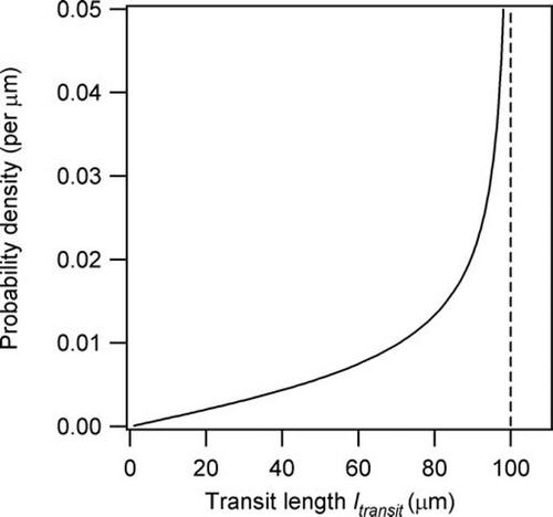
Figure 6 shows a plot of this theoretical function. Most transits have a length l _transit close to the maximum possible length, D _transit, while the probability of short l _transit is quite low. This is also depicted schematically in Figure 5, which shows a number of droplet trajectories through the view volume. In practice, for each droplet that crosses the view volume, the time spent in the view volume (termed the transit time, t _r ) is recorded. From this, l _transit is calculated simply using:

where u is measured on a single drop basis (Equation [2]). Given a population of monodisperse drops of size d, one can plot the distribution of l _transit values, and fit these data to the theoretical distribution function by varying the unknown parameter D _transit. In fact, it is easily shown that, assuming a circular cross section, the probability distribution function P is described by the equation:

The best-fit value for D _transit yields D _beam for drops of size d, assuming D _transit = D _beam (i.e., assuming the laser has a circular cross section).

FIG. 6 Theoretical PDF of l _transit given by Equation (5) plotted as solid line, where the specified view volume diameter is 100 μ m (dashed vertical line).

This fitting is then repeated for a range of d, from which we can determine a theoretical function for D _beam(d) given the following assumptions: (1) we assume that the laser cross section has a Gaussian intensity distribution, (2) we assume that to trigger the gate of the instrument (which identifies the passage of a drop through the measurement volume), a minimum signal power must be scattered by that drop and received by the photodetectors, and that this value is independent of d, and (3) we assume geometric light scattering is applicable. Given these three assumptions, we derive a theoretical prediction for the dependence of D _beam on d:

where K ₀ and K ₁ are constants. In the next section, we compare these theoretical predictions with values determined during aircraft measurements of marine stratocumulus clouds using the Artium F/PDI.

2.4. Comparison of Theoretical and Measured View Volumes

We now perform comparisons of the theoretical view volume behavior with that for F/PDI. This will occur in two steps: (a) we first test the theory that D _beam for a nearly monodisperse population is distributed according to Equation (5) and illustrated in Figure 6; (b) we then test to see if D _beam depends on d according to Equation (6). For these comparisons, we will utilize data collected during the Marine Stratus Experiment (MASE) conducted over the eastern Pacific in the vicinity of Monterey, CA. The data used are from July 10, 2005 when substantial marine stratocumulus were sampled by the CIRPAS Twin Otter. During this flight, constant-altitude legs were flown just above cloud base, within the cloud, and just within cloud top. A total of ∼ 50 min of in-cloud data (averaged to 1 s) were obtained.

To calculate D _beam(d), we use the following procedure:

1.	Select all drops within a narrow range of sizes. Bin widths are fixed geometric width, with d n + 1/d n = 1.122, where d n is the mean diameter of bin n. The size range of drops for which substantial data was obtained is 12 μ m to 70 μ m diameter, yielding 15 drop size bins. Absolute bin widths are therefore < 2 μ m at the low end of the size range, up to ∼ 7 μ m at the largest sizes.
2.	For each drop in a given size bin, we calculate l transit, where gate time and transit velocity are both recorded for that drop, according to Equation (4).
3.	From the entire population of observed drops in the size bin, a probability distribution function (PDF) of l transit is generated.
4.	This PDF is fit to the theoretical function given in Equation (5), where the fitting routine has one free parameter, D transit. This yields D beam for this size range assuming that the beam is circular, i.e., D beam = D transit.
5.	Repeat Steps 1 to 4 for all size bins in the range of interest. This generates D beam(d) for all d in the size range of interest.
6.	We check to see if D beam(d) from Step #5 depends on d according to the theoretical prediction given by Equation (6). If so, then this gives us strong confidence that the instrument is performing in a way that agrees with our theoretical understanding, and that the assumptions that we made in generating Equation (6) is consistent with the observations.

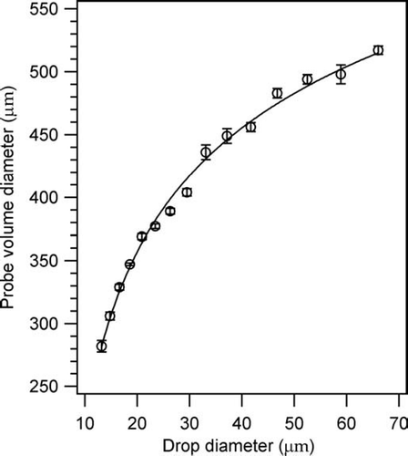
Results from Step 6 are shown in Figure 7 and shows that theory does an excellent job in fitting the data, which strengthens our belief that the instrument is behaving as theory predicts, and reinforces our belief that the view volume determination method is works well. This fitted curve for D _beam(d), along with L _aperture, defines the instrument view volume. Once these two parameters have been derived, then Q _sample is calculated from Equation (3), after which the drop size distribution can be determined, which is the ultimate goal.

FIG. 7 Data points are the fitted PVD values for each size range. Error bars are the 1 σ uncertainty in the fitted PVD. The fitted curve is the theoretical dependence of PVD on d from Equation (6), where K ₀ and K ₁ are fitting parameters. The theoretical curve fits the data very well, indicating that the instrument performance is consistent with our theoretical understanding.

2.5. Potential F/PDI Uncertainties for Droplet Size and Concentration

There are a number of possible ways in which uncertainty in the resulting measured drop size distribution can occur. We will document these here, and note that they apply to the instrument intercomparisons described next (Section 3).

Multiple Triggering

It is possible that one drop triggers the gate (which signals the presence of a drop in the view volume) more than once. This could lead to multiple counting of that drop. A typical event has one or more of very short gates (which if real would signal a very short duration passage of a drop through the view volume) on either side of the actual drop passage. Noisy environments are more prone to causing such events, since the detector will sometimes trigger on noise spikes. Such problems can be reduced if not eliminated by careful selection of the signal processing settings, such as using proper filters. In addition, such events can almost always be detected and rejected in post-processing based on minimum signal duration and inter-droplet arrival time distributions.

Coincidence

As for all single particle instruments, the coincidence of multiple particles within the instrument view volume can yield an erroneous measurement. This problem increases as the drop concentration increases. If two similarly sized drops are coincident, it is most likely that the instrument electronics will reject both drops because the Doppler burst and phase differences will not appear as that from a single drop. If, however, two drops of very different size are coincident, the most likely scenario is one where the signal from the large drop overwhelms that from the small drop, and the large drop will be detected while the small one is missed. Thus, under-counting of the most common drops in a cloud can occur, but the larger, rarer drops will be counted accurately. Note that one problem faced by the FSSP is mistaking two small coincident drops for a single larger drop (Cooper 1988), which cannot happen with the F/PDI. Furthermore, the sample volume can be easily reduced to minimize coincidence errors. A Poisson statistical analysis based on the droplet interarrival times can be used to estimate the probability of coincidence occurrences. It is possible to theoretically correct for coincidence counting errors based on measured size distributions, although we have not yet implemented such an algorithm.

Dead Time

Modern electronics have mostly eliminated dead time issues from aircraft single particle probes; the F/PDI has no dead time.

Optical Contamination

Over the course of a flight, contamination of the optics, primarily the outside windows, can be a problem. This problem is minimized when the instrument commonly flies through clouds (which is the primary focus of the instrument), since impacted cloud drops can wash contaminates from the vulnerable external surfaces. However, because drop size measurements depend fundamentally on frequency rather than intensity magnitude, any moderate reductions in the intensity of the transmitter beam or scattered signal do not significantly affect the sizing of the drop provided that there is sufficient signal for drop detection. In principle, this means that the lower size limit for detection increases with contamination, and the view volume may decrease as well. The latter effect can be detected by performing view volume analyses described in section 2.4 for, e.g., the first and second halves of a flight separately. If D _beam(d) does not change, then this implies that contamination was not a problem. Also, the detector gain can be increased to partly compensate for the loss in signal amplitude.

Drop Sizing Checks

One useful check of the drop size measurements is the velocity data. On an aircraft, the true air speed can be checked against the mean cloud drop speed passing through the view volume. The latter depends on the fringe spacing δ, which in turn also affects the drop size. Therefore, any problems with the δ calibration will be seen in the velocity data. If these velocities agree, then this implies that δ is accurately known, and thus gives confidence in the drop size measurements as well, which depend on the fringe spacing. In principle, any discrepancy in the velocity data can be used to correct the drop sizes, since the correct value of δ can be inferred and then used to re-process the raw data to yield more accurate drop sizes. Drop diameter d depends linearly on phase difference for drops in the geometric optics regime, and thus the correction at most drop sizes is linear and thus simple to implement.

Drop Sizing Uncertainties

Other parameters that affect drop sizing, primarily the receiver spacing, can not be checked in this way, and therefore rely on the instrument calibration. Note that this spacing is fixed, and therefore only one calibration is required unless the optical hardware is physically moved, which is extremely unlikely to occur during aircraft operation. A phase calibration is performed on a regular basis to account for differences in electronics for each detector channel which could otherwise generate an artificial phase difference between two signals, e.g., detectors A and B in Figure 2. A typical phase difference is 2°, with a standard deviation of ∼ 0.5°. Even assuming a full 2° uncertainty in phase difference, this represents a ∼ 0.2 to 0.4% uncertainty in size, since the functional range in phase difference is approximately between 1.5 and 3 × 360°, i.e., between 540° and 1080°. With a full-range drop size of 150 μ m, this is a 0.3 to 0.5 μ m uncertainty in size. More realistic phase difference uncertainties lead to estimates lower by roughly an order of magnitude. Thus, phase calibration is unlikely to be a significant source of error as compared to other potential sources.

Trajectory Errors

When a drop whose size is comparable to or larger than the beam diameter passes through the view volume, significant errors in sizing can arise. This occurs in this case if reflection and refraction both contribute significantly to the scattered signal. For the case of the F/PDI, the beam diameters derived in Figure 7 are much larger than the drops of interest and therefore this is not a significant problem. Furthermore, logical tests have been incorporated into recent updates of the instrument software that eliminate these errors.

3. INSTRUMENT INTERCOMPARISONS

3.1. Liquid Water Content Comparisons

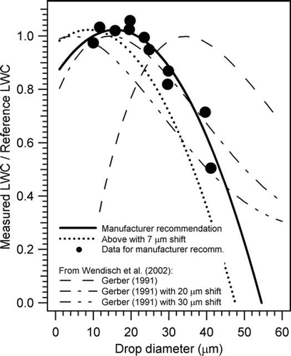
Once D _beam(d) has been determined, drop number distributions and mass distributions can be calculated. The performance of the F/PDI for measuring liquid water content may be evaluated by integrating the mass distributions and comparing them with a Gerber Scientific Inc. PVM-100A (Gerber et al. 1994) which provides total liquid water content (LWC). The data set used is the same July 10, 2005 case from MASE described above. The PVM-100A was mounted on the fuselage of the Twin Otter, ∼ 5 m from the location of the F/PDI. One important characteristic of the PVM probe is that its sampling efficiency decreases at large drop sizes (Gerber et al. 1994; Wendisch et al. 2002). Figure 8 shows a number of PVM sampling efficiency curves. We initially used the curve labeled “Manufacturer recommendation” which is the curve recommended by Gerber Scientific, Inc. This curve is based on the data set shown, which is a composite of measurements utilizing a cloud chamber, glass beads and aircraft observations. In order to properly compare F/PDI-derived LWC with that measured by the PVM, this roll-off must be accounted for by multiplying the derived liquid water in each PDI size bin by the appropriate efficiency.

FIG. 8 Comparison of various LWC efficiency curves for the PVM-100A.

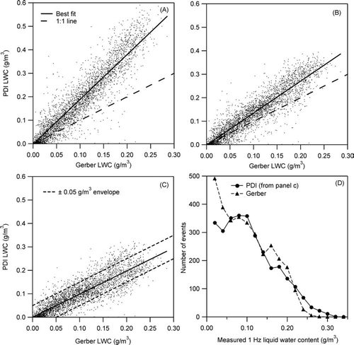
Figure 9 shows three different comparisons of 1 Hz liquid water contents derived from the F/PDI and PVM (hereafter LWC _PDI and LWC _PVM , respectively). Panel A shows all data where no correction has been applied to LWC _PDI , in which case LWC _PVM is much lower than LWC _PDI . This occurs because the measurements are from fairly clean stratocumulus, where there is an appreciable concentration of drops as large as 70 μ m, which is above the PVM detection limit (Figure 8). In panel B, the manufacturer recommended efficiency curve is applied to the LWC _PDI data. The resulting relationship is LWC _PDI = 1.36 * LWC _PVM , i.e., the PDI measures 36% more LWC relative to the PVM. In panel C, the Gerber efficiency curve has been shifted downwards by 7 μ m diameter (this shifted curve is plotted in Fig. 8); with this shift, LWC _PDI = LWC _PVM in the mean. Panel C also displays lines denoting uncertainties of ± 0.05 g/m³, which contains 85% of the points. We now explore possible factors that could lead to this discrepancy, although we note that uncertainties in PDI sizing are one possible explanation, as detailed in Section 2.5.

FIG. 9 Comparisons of PVM-100A LWC (“Gerber”) measurements with PDI-derived LWC. Each data point corresponds to 1 s of measurement time. (a) PDI LWC for entire PDI size range (drops 3 to 150 μ m) is computed. (b) PDI LWC is computed using the most recent PVM-100A efficiency curve (see text), which exhibits a 50% sampling efficiency at ∼ 40 μ m. (c) Like (b), except the PVM correction curve is shifted towards smaller drop sizes by 7 μ m diameter, which is the shift necessary to match PVM-100A and PDI LWC. (d) Frequency distribution of 1 Hz LWC measurements from both probes. The PVM-100A has 3186 s of data, while the PDI yields 2956 s of data, a difference of ∼ 8%.

Wendisch et al. (2002), hereafter WGS02, performed numerous wind tunnel tests using the PVM, and concluded that their results best fit either the Gerber (1991) efficiency curve shifted by 20 μ m or 30 μ m, depending on the test (Figure 5a and Figure 5b, respectively, from WGS02), as shown in Figure 8. Notice that the manufacturer curve shifted by 7 μ m falls in between the two WGS02 curves up to a drop size of 35 μ m (after which it drops to zero much more abruptly). Thus, it is possible that one explanation for LWC _PDI being larger than LWC _PVM is that the manufacturer efficiency curve rolls-off at a drop size that is too large, and that including the 7 μ m shift better represents the actual PVM performance, a conclusion that is consistent with WGS02. We note that analyses of other MASE flights consistently yields the same 7 μ m shift to bring the PVM and PDI LWC values into agreement. However, the results from WGS02 also suggest that there is not a single efficiency curve, since the same experimental method in two different environments led to best-fit curves that are separated by 10 μ m. Thus, one interpretation of WGS02 is that the PVM efficiency curves vary depending on other factors (for example, breadth of the drop size distribution) besides simply drop size, and that under the conditions encountered during MASE, a 7 μ m shift in the original manufacturer curve is appropriate. Alternatively, it is possible that the PDI derived drop sizes and/or concentrations (the latter depending on the view volume) are biased such that they lead to high LWC _PDI relative to LWC _PVM , for reasons addressed above (Section 2.5). The available data set is insufficient to determine with any certainty which of these explanations (if any) is correct. It is likely, though, that incorporating multiple data sets from different environments would help lend insight into this problem, which we defer to future work.

Panel D in Figure 9 shows the frequency distribution of 1 Hz LWC _PDI and LWC _PVM for the entire flight, where the LWC _PDI data used is from panel C (i.e., derived using an efficiency curve shifted by 7 μ m). Because the instruments are not perfectly co-located, and they might not be perfectly time synchronized, it is unreasonable to expect that two identical instruments would yield a 1 Hz scatter plot such as panel C to exhibit perfect agreement. However, for a sufficiently long sampling time in a relatively homogeneous environment such as a solid stratocumulus deck, it is more reasonable to believe that two identical instruments would yield statistically identical LWC distributions over the course of the flight. Panel D shows that the PVM sampled a larger number of low LWC (< 0.05 g/m³) events over the course of the flight. We attribute this to the larger view volume of the PVM, which should record events with such low LWC that the F/PDI, with its smaller view volume, will not register any drops at all. This is an intrinsic difference between single-drop and population-integrating instruments. In the LWC range of 0.05 to 0.15 g/m³, the two instruments agree remarkably well. In the large LWC range, however, it appears that the PVM-100A identified more events in the range 0.15 to 0.2 g/m³, whereas the F/PDI identifies more events in the 0.2 to 0.3 g/m³ range, with the discrepancy in the number of events being quite similar in these two ranges. This observation is again consistent with the idea that the PVM-100A probe is in fact missing some larger drops from events that belong in the 0.2 to 0.3 g/m³ range, and instead measuring LWC to be between 0.15 and 0.2 g/m³. If this is true, it suggests that the roll-off used in panel C, which is already shifted to smaller drop sizes by 7 μ m, may still be inadequate. Note that this does not affect the best fit curve (panel C) because these events represent a relatively small fraction of 1 Hz events analyzed.

We conclude that the comparison of measured LWC using the PVM-100A and the F/PDI yields fairly reasonable agreement, albeit with some biases which fall within the bounds of prior documented uncertainties of these measurements.

3.2. Drop Size Distribution Comparisons

Eventually it would be in the best interest of the droplet measurement community to make a thorough intercomparison of the F/PDI with other cloud drop size distribution probes (e.g., FSSP, Fast-FSSP). Carrying out a meaningful intercomparison is a significant undertaking and will require a dedicated, collaborative effort between groups with the various instruments. The ideal experiment would be one where a known drop size distribution standard were used to challenge such instruments under conditions relevant to aircraft sampling of clouds, i.e., similar velocity, drop concentration and size range. Even relative comparisons (i.e., in the absence of such a standard) of the performance of the F/PDI with, e.g., FSSP, represent a very substantial amount of work in order to understand the fundamental source of any differences in performance that are observed during cloud sampling. Furthermore, relative comparisons inevitably are plagued with the ambiguity as to how close either instrument is to measuring the true size distribution. Recognizing the great importance of carrying absolute comparisons of size-distribution instruments, or at least intercomparison under controlled conditions, we defer such an extensive study to the future.

For the purposes of gaining some initial insight into the performance of the F/PDI as compared to the FSSP (the instrument most frequently used by the community for size distribution measurements), we again show data from MASE (data from July 16, 2005, although data from many other MASE days are qualitatively very similar). During MASE, an FSSP-100 was flown simultaneously with the F/PDI on-board the CIRPAS Twin Otter, albeit on the opposite wing (separation ∼ 10 m). The FSSP is well-maintained, with frequent checking, cleaning and calibration during all field programs by CIRPAS facility scientists. These FSSP measurements have been used by numerous investigators during MASE (Lu et al. 2007). For all the below comparisons, there is no absolute standard for the measurements, and therefore there is no clear way to determine which instrument measures values closer to the truth. We therefore seek to describe the differences in performance without ascribing relative success or failure to either instrument.

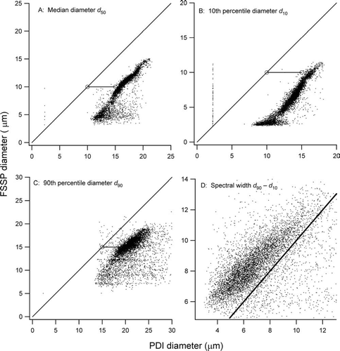
Figure 10 shows a comparison of the F/PDI and FSSP measured drop size distribution parameters, specifically the 10th, 50th (or median), and 90th percentile diameters (hereafter d ₁₀, d ₅₀, and d ₉₀) for these distributions, as well as d ₉₀–d ₁₀, which is one measure of the distribution breadth. From these plots, it appears that there is a ∼ 5 μ m discrepancy between the measured distributions, which is reasonably consistent among all the distribution parameters, although the discrepancy is greater for d ₁₀ than it is for d ₉₀. The discrepancy in the breadth of the distribution in linear space as measured by d ₉₀–d ₁₀ is ∼ 2 μ m (compared to a total width varying from 4 to 10 μ m), with the FSSP tending to measure broader distributions by 20 to 50% than the F/PDI.

FIG. 10 Comparisons of the shape of the drop size distribution as measured by the F/PDI and a FSSP-100. Panels A, B, and C represent the d ₅₀, d ₁₀, and d ₉₀, respectively, for the measured size distributions. In each of these panels, the line terminated by two circles represents 5 μ m. Panel D represents d ₉₀–d ₁₀. In all panels, a 1:1 line is drawn. Each dot represents 1 s of data. Approximately 7000 s worth of data is shown.

These parameters, however, do not address the absolute concentrations of the size distribution. An alternate and complementary way of comparing the F/PDI and FSSP is to look at the measured concentration in particular size ranges. Figure 11 shows such a comparison, where the entire FSSP size range (ignoring the first bin, which is generally considered unreliable) has been broken up into 6 size bins, and the F/PDI measurements are sampled to match these size bins with a 5 μ m shift in size, i.e., a 15 μ m drop measured by the F/PDI will be considered a 10 μ m drop for this comparison, as suggested by Figure 10. The F/PDI data were shifted to smaller sizes because this was much more convenient than doing the converse for the FSSP sizes, and is not intended to suggest that F/PDI size data are actually biased in this way. The same comparisons performed without such a size shift (not shown) yielded comparisons that were generally extremely poor.

FIG. 11 Comparison of the measured drop number concentration by the F/PDI and FSSP in six different nominal size bins. In all cases, the F/PDI distributions have been shifted towards smaller size by 5 μ m to account for the sizing discrepancy shown in Figure 10. This was more convenient than shifting the FSSP distributions upwards by the same amount, and is not meant to imply that these represent the actual drop sizes.

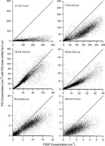
For the five largest size bins shown in Figure 11, there is a good correlation between FSSP and F/PDI concentrations. In general, the FSSP infers higher concentrations than the F/PDI, with typical differences on the order of a factor of 2, but as small as ∼ 20%, depending on the size bin. The agreement between FSSP and F/PDI data does not appear to systematically depend on either drop size (e.g., it does not simply improve as drop size increases) or drop concentration (e.g., best agreement is not for the smallest or largest concentrations). For the smallest size bin (2.1 to 7.3 μ m), the FSSP predicts drop concentrations about an order of magnitude higher than the PDI. One possible explanation for this discrepancy is that the FSSP was triggering on noise, yielding numerous false drops in the smallest size bin. This is a well-known problem of the FSSP, which is normally dealt with by ignoring the lowest FSSP channel, which we have also done here. This analysis perhaps indicates that the noise problems extend to higher FSSP channels, at least in this data set. Whether this problem can extend to the other size bins and lead to an FSSP overcounting in those comparisons as well is unknown. It is also possible that uncertainties in PDI counting or view volume are partly responsible for these discrepancies, as discussed above (Section 2.5).

Overall, we find the correlation in the size-dependent concentration measurements encouraging, but acknowledge that the differences in performance between these instruments are substantial. Without a controlled experiment with known size distribution, and in the absence of an accepted standard instrument for size distribution measurements, it is not possible to determine which instrument measures more realistic size distributions. The results of this intercomparison clearly indicate that further instrument evaluation under controlled conditions with a known size distribution or an accepted standard is necessary to draw further conclusions.

4. TURBULENCE MEASUREMENTS

Clouds are inherently turbulent due to strong buoyancy and shear production associated with convection, latent heat release, and radiation. Unfortunately, however, it has been a challenge to obtain reliable measurements of turbulent velocities in clouds. Traditional methods such as sonic anemometry or differential pressure measurements have rather low spatial resolution at aircraft flight speeds, and implementing the classic high-resolution method of hotwire anemometry is challenging because of the presence of water droplets and other particles in the flow (Siebert et al. 2007). The few high-spatial resolution cloud measurements that have been made suggest that turbulence follows the classic energy cascade scaling for velocity (e.g., Siebert et al. 2006a; see Section 4.1 for a brief overview of the energy cascade). Given the growing recognition that turbulence plays an important role in cloud microphysical processes (e.g., Vaillancourt and Yau 2000; Shaw 2003), however, it is important to characterize fine-scale properties of turbulence as a regular aspect of cloud field experiments. The purpose of this section is to describe the capabilities of the F/PDI for obtaining turbulent velocity measurements in clouds. Laser Doppler anemometry has been used extensively for turbulence measurements within the engineering community and is a well documented technique (e.g., Albrecht et al. 2003), but there are aspects of the instrumentation and data that are unique to the cloud physics implementation and, in particular, the airborne aspects typical in such work. In Section 4.1 we provide an overview of the basic principles with emphasis on the measurement of turbulence in clouds and the attainable resolution for typical cloud conditions. Sections 4.2 and 4.3 deal with two possible sources of bias that must be carefully considered: the determination of fluid (air) velocity given that the actual measurement is of droplet velocity, and the influence of the instrument housing itself on the measured velocity, respectively. Finally, in Section 4.4 the F/PDI is compared to two other measurement methods for turbulent velocity.

4.1. Basic Principles

The utility of the phase Doppler technique for cloud studies is greatly enhanced because it provides not only a droplet size distribution, but also measures simultaneously each droplet's incoming-velocity (the velocity component perpendicular to the optical axis and in the plane of the crossed beams; cf. Figure 2). The resulting time series of droplet incoming-velocity component (hereafter abbreviated simply as “velocity”) can be analyzed to obtain in-cloud turbulence statistics such as power spectral densities and turbulent kinetic energy dissipation rates. For airborne applications, the spatial and temporal resolution of PDI is significantly higher than is possible with typical differential-pressure methods, and therefore the range of eddy sizes that can be resolved within the turbulent energy cascade is extended. Furthermore, the method is ideally suited for cloud measurements because by definition it requires the presence of particles in the turbulent flow.

Under many cloud conditions, PDI instruments can be configured to provide a high-spatial-resolution data series, with the resolution determined by the droplet arrival rate (each droplet is associated with one velocity measurement). For example, assuming cloud droplets are uniformly distributed with number density n and that the instrument has measurement cross section σ, the average spacing between sampled droplets is l ≈ (nσ)^{− 1}. An instrument sample volume with linear dimension of 400 μ m sampling a cloud with n = 500 cm⁻³ results in l ≈ 1 cm, compared to spatial resolutions of several meters or more for airborne velocity measurements based on differential-pressure probes. In practice, the spatial resolution for turbulence statistics is not exactly what is implied by the average droplet spacing l because velocity measurements are not uniform in time, but rather are associated with the random arrival times of individual droplets. As a result special data processing methods must be used, which tend to limit the usefulness of the calculated statistics (e.g., power spectra) to scales above approximately 10 l. The most commonly used method is sample-and-hold reconstruction. Essentially, the velocity data series is resampled at a frequency much higher than the mean droplet arrival rate. The velocity value at each sample point is taken to be the closest prior measured velocity. This method is preferred, apart from its simplicity, because it has an associated error that is well understood, and therefore allows for a partial correction (e.g., Benedict et al. 2000). More complicated schemes such as linear interpolation are found to provide no significant improvement while introducing errors whose characteristic and correction scheme are not well understood. These and other approaches to power spectrum estimation are described in the review article by Benedict et al. (2000).

Given an estimate of the spatial resolution, we can ask what corresponding velocity resolution will lead to an optimal measurement (i.e., spatial and velocity resolutions should be consistent, with neither limiting the subsequent analysis). Because the application here is to atmospheric flows, attention will be focused on measuring turbulent velocities. Turbulence is a multi-scale process in which energy injected at large scales (of order 10 to 100 m for typical cloud conditions) “cascades” to progressively smaller scales through nonlinear interactions such as vortex stretching. Over most of these spatial scales, known as the inertial range, viscous forces are negligible compared to fluid inertia. The scales at which viscosity becomes important lie in the dissipation range, characterized by the Kolmogorov microscale (of order 1 mm for typical cloud conditions). The inertial range therefore consists of velocity fluctuations, or eddies, with spatial scales spanning four to five decades. (An overview of the energy cascade and the related length and time scales can be found in the text of Kundu and Cohen (2004, Chap. 13), and more thorough discussions in, for example, the text by Davidson (2004).) The standard picture of the energy cascade suggests that the velocity fluctuation scale u _r associated with spatial scale r within the inertial range is u _r ∼ (ϵ r)^1/3, where ϵ is the turbulent kinetic energy dissipation rate. Typical cloud energy dissipation rates of 10^{− 4} ≤ ϵ ≤ 10^{− 2} W kg⁻¹ therefore result in 2 ≤ u _r ≤ 10 cm s⁻¹ for r = 10 l = 10 cm. Ideally, therefore, the PDI instrument should be capable of resolving similar velocity magnitudes.

As described in Section 2.2, PDI obtains the velocity of each sampled droplet by measuring the corresponding Doppler difference burst frequency through the relation ƒ _D = u/δ (Equation [2]). The frequency estimation is done essentially via a discrete Fourier transform method. Neglecting the low frequency modulation on the Doppler bursts (resulting from Gaussian beam intensity profile of the probe volume) and assuming sampling noise with a white spectrum (this implies that the accuracy of the measurement is sampling limited, discussed below), the uncertainty in the frequency measurement can be derived from estimation theory to have a theoretical (Cramer-Rao) lower bound given by (Albrecht et al. 2003, Sections 6.1.5 and 6.3)

Here A is the amplitude of the Doppler burst signal, σ _n is the measurement noise (including detector shot noise, etc.), N is the number of data points sampled by the instrument within each burst, and ƒ _s is the sampling frequency. The frequency uncertainty Δ ƒ _D determines the droplet velocity measurement precision; note, however, that there may also be velocity biases due to uncertainties in the optical parameters that yield the estimate of the fringe spacing δ, although such bias is negligible compared to the overall uncertainty. A conservative estimate of Δ ƒ in this work can be obtained by assuming a signal to noise ratio of SNR ≈ (A/σ _n )² = 1, a minimum burst sample size of N = 64, and a sampling frequency ƒ _s = 10 MHz. Regarding the latter, in setting up the processor parameters the Nyquist criterion is used to adjust the sampling frequency to correspond to the dynamic range of the velocity measurement (i.e., the dynamic range is adjusted to account for the anticipated range of velocities to be measured). The ratio 2Δ ƒ _D /ƒ _s is equivalent to the velocity measurement error relative to the velocity dynamic range, which for the numbers given above is 0.003. For a maximum velocity of 100 m s⁻¹ this results in Δ u ≈ 30 cm s⁻¹. In practice it is more common to have SNR ≈ 10 and N ≥ 128, so the resolution will be higher. Furthermore, when the platform velocity is relatively constant the range of velocities is narrow and thus the processing can be optimized for a narrow frequency band. For example, the range of velocity needs to be set wide enough to account for rms turbulence velocity fluctuations and any variations in platform velocity. In general, it is possible to optimize instrument settings to obtain 2Δ ƒ _D /ƒ _s better than 0.1%.

The use of the Cramer-Rao lower bound implicitly assumes that the measurement is sampling limited under white noise. This can be seen more clearly if we rewrite Equation (7) in terms of ƒ _D ,δ, SNR, and beam diameter D _beam, by using N = t _r ƒ _s with transit time t _r = D _beam/u, and by assuming N ² ≫ 1:

The relative accuracy of a velocity signal, therefore, can be improved by increasing signal to noise ratio (e.g., increasing laser power or lower-noise detectors), by decreasing the fringe-spacing to beam-waist ratio (noting, however, that the beam waist is dependent on the SNR through laser power), or by increasing the sampling frequency. This apparently implies that one may improve the measurement accuracy indefinitely by increasing ƒ _s , but this cannot be done indefinitely for several reasons. First, our implementation of the real-time signal processing limits the number of samples to N ≤ 1024. Second, at some point the measurement accuracy would be limited by other errors unaccounted for in the development of the Cramer-Rao theory (e.g., the non-constancy of droplet velocity traversing the probe volume). Third, a more fundamental limit to the Cramer-Rao error estimate can be seen by noting from the last term in Equation (8) that (Δ ƒ _D /ƒ _D )∼ 1/√N, consistent with the averaging of independent samples. Any real noise process will in fact not be perfectly white, and therefore will have a finite correlation time τ _c . When ƒ _s > τ _c ^{− 1} the samples are no longer independent and therefore the fundamental white noise assumption for Equation (8) is invalid.

The Δ u estimated from Equation (7) is approaching the u _r ≈ 10 cm s⁻¹ target for r = 10 cm, and we recall that this analysis is based on a conservative estimate of signal to noise ratio, etc. The velocity resolution is therefore reasonable for typical cloud measurement conditions, and certainly several steps can be taken to improve upon this if velocity measurements are the primary goal. The spatial resolution of the measurement and the velocity resolution taken together show that PDI has the potential to resolve a significant portion of the inertial range of the turbulent energy cascade in clouds (assuming the dissipation range begins at approximately 10η ≈ 1 cm, where η is the Kolmogorov scale). It should be pointed out, however, that for airborne applications there is an inherent dependence of Δ u on the flight velocity U. Assuming U > > u _rms such that ƒ _D ≈ U/δ, and the fact thatΔ u = Δ ƒ _D δ we find from Equation (8) that the velocity uncertainty scales with flight velocity and beam parameters as:

(note that Nyquist sampling was also assumed here). Under typical operating conditions, therefore, it is advantageous to use the minimum possible flight velocity in order to obtain maximum resolution in turbulence velocity statistics.

4.2. Measurement of Droplet Versus Fluid Velocity

An aspect of obtaining turbulence statistics from PDI instruments that must be considered is the fact that droplet velocities, not fluid velocities, are measured. Intuitively one would expect that the droplet motion may deviate from that of the background air due to the difference in the mass density of the two phases. To obtain reliable turbulence statistics it is necessary to use velocity data only from droplets sufficiently small to follow fluid pathlines (Bachalo 1997). A cutoff can be obtained by considering the frequency response of a droplet in an oscillating background fluid (e.g., Albrecht et al. 2003, Section 13.1), resulting in slip velocity s = (u _ƒ − u _d )/u _ƒ, where u _d and u _ƒ are the droplet and fluid velocities, respectively. For clouds, where the droplet density ρ _d is much greater than the fluid density ρ_ƒ, the droplet slip velocity is

where τ _d = ρ _d d ²/(18ρ_ƒ ν) is the droplet inertial time scale, ν is the fluid kinematic viscosity, and ƒ _r is the fluid oscillation frequency. The fluid oscillation frequency relevant to this problem should be estimated as the inverse of the Lagrangian velocity correlation time in the particle frame of reference (Bachalo 1997). Obtaining such a quantity remains an outstanding problem in the study of turbulence, however, so it is often estimated from the Eulerian fluid oscillation frequency. The latter depends on the spatial scale r to be resolved within the turbulent energy cascade, such that ƒ _r = τ _r ^{− 1}≈ (ϵ/r ²)^1/3. In relation to our measurement in cloud we assume an acceptable slip of s = 0.01 at a spatial scale of r = 0.1 m and an energy dissipation rate of ϵ = 10^{− 2} W kg⁻¹, resulting in d ≈ 80 μm as the maximum allowable droplet diameter. Such droplets, however, would have appreciable fall velocities. Therefore, we should apply a similar frequency response model to a droplet falling through a spatially varying (but frozen) fluid velocity field. For a droplet falling through eddies of size r at terminal velocity τ _d g, the relevant frequency is ƒ _g = τ _d g/r, and in this case the 1% slip size is reduced to d ≈ 60 μ m.

4.3. Modeling of Flow Around the Instrument

To conduct accurate in situ measurements within any fluid, it is important that the ambient flow not be disturbed by the instrument housing. This is of special importance in studies of turbulence and particle spatial distributions, but is also relevant to preventing biases in the cloud drop size distribution measurements due to differing droplet inertia or droplet shattering. Typical applications of phase-Doppler interferometry in engineering flows have the optics and detectors positioned outside of the flow, with the flow itself confined to a chamber or device. In its application to cloud measurements, however, it is more convenient to have a self-contained instrument that is placed in the flow itself. This places greater constraints on the instrument housing design, but allows benefits of flexibility and the ability to deploy on different platforms. For example, the F/PDI has been deployed on various research aircraft (including the CIRPAS Twin Otter and the NCAR C130), on a helicopter-borne instrument payload (ACTOS), and in large research wind tunnels (Cornell DeFrees active grid wind tunnel and the NASA Icing Research Tunnel).

The F/PDI instrument housing has been designed to avoid significant flow distortion for flow speeds ranging from those existing in wind tunnels or ground-based experiments to typical aircraft flight speeds. (Actual design requirements are that the mean flow speed is above several centimeters per second and that the direction of the incoming flow is within approximately 10 degrees of normal.) The general flow pattern on the upstream side of the instrument, where the sample volume is located, is determined (1) by the boundary-layer thickness and (2) by the approximately-irrotational flow field outside the boundary layer. Regarding item (1), boundary-layer thickness obeys known scaling laws for both laminar and turbulent flows (e.g., Kundu and Cohen 2004, Chap. 10), becoming thinner with increasing flow speed. The absolute boundary layer thickness at the window region is always less than several millimeters, and therefore is very far from the measurement volume. Regarding item (2), the velocity field outside the boundary layer can be assumed to be irrotational, such that the velocity perturbation relative to the mean background velocity only depends on the geometry of the body (result valid for simple bluff bodies; Kundu and Cohen 2004, Chap. 6). Therefore, as the mean speed is increased from wind-tunnel speeds to typical flight speeds, the irrotational flow pattern around the instrument is not changed significantly and characterizing the flow pattern at one relative speed is sufficient.

The detailed flow around the instrument housing, assuming normal incidence, has been simulated using the commercial Fluent computational fluid dynamics package. The computational grid was constructed using exact instrument dimensions, with the exception of fine details around the windows, and was appropriately refined to resolve boundary layers. Results were calculated for a mean flow speed of 2 m s⁻¹, representative of a research wind tunnel, but as just discussed, are representative of those present for flight speeds of 50 to 100 m/s (e.g., always assuming incompressible flow, with non-separated boundary layers). The Fluent simulations demonstrate that the velocity field near the sample volume is only slightly perturbed due to the pressure field resulting from the essentially irrotational flow outside of the boundary layer. Hotwire anemometer measurements in a wind tunnel and comparison with other airborne velocity measurements (see below) confirm these general conclusions. Finally, calculations of particle trajectories were also conducted using Fluent. The quantitative results confirm that velocity deviations and relative particle positions are always well under 10% of their undisturbed, upstream values.

4.4. Comparisons with Other Instruments

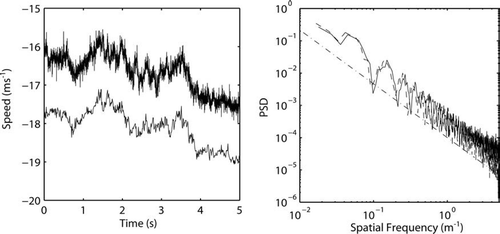
An example of turbulence data obtained from a PDI instrument flown in cloud is given in Figure 12. Simultaneous data from a sonic anemometer are shown for comparison. Note that the performance of the sonic anemometer in clouds has been characterized and found to be reliable (Siebert and Teichmann 2000). The measurements were made aboard the Airborne Cloud-Turbulence Observation System (ACTOS) deployed via helicopter (Siebert et al. 2006). The left panel in Figure 12 shows 5-second time series from the PDI instrument and the sonic anemometer. There is an offset of approximately 1.5 m s⁻¹ due to the location of the PDI instrument near the stagnation point of the ACTOS payload, but otherwise the agreement is reasonable. (The ACTOS payload has a cross section with linear dimension approximately 50 cm and the F/PDI was located approximately the same distance from the payload flow blockage; assuming irrotational flow around a buff body such as a hemisphere, the flow disturbance at this distance is roughly 10%, consistent with the observed offset.) For these measurements the fringe spacing was δ = 14.7 μm and the beam waist was approximately D _beam = 250 μ m, which from Equation (8) gives Δ ƒ _D /ƒ _D ≈ 4× 10^{− 3}, or a typical velocity uncertainty of approximately Δ u ≈ 10 cm s⁻¹. Power spectra of a longer time series from the same cloud are shown in the right panel, and again there is reasonable agreement between the two instruments throughout the resolvable subset of the inertial range. Furthermore, both power spectra match, at least to within the sampling uncertainty, the expected − 5/3 power law dependence (exemplified by the dashed curve) for power spectral density of the longitudinal velocity component within the inertial range (e.g., Davidson 2004). The power spectra are plotted up to a spatial resolution of 20 cm (spatial frequency 5 m⁻¹), which is approximately the limit (10 l) of the sample-and-hold method used for the selected segment of PDI data, as well as the spatial resolution of the sonic anemometer. The slight flattening of the PDI power spectrum at high frequencies is characteristic of the sample-and-hold method.

FIG. 12 Left panel: Measured velocity versus flight time for F/PDI (top curve) and a sonic anemometer (bottom curve). The offset of approximately 1.5 m s⁻¹ is due to the location of F/PDI being closer to the stagnation point of the measurement platform than the sonic. Right panel: Power spectral density (PSD) versus spatial frequency for flow velocity measurements from F/PDI (solid) and the sonic (dashed); a line with slope –5/3 is included for reference (dotted).

A second data example to demonstrate the reliability of the PDI for detailed turbulence measurements is shown in Figure 13, which shows second- and third-order structure functions for the longitudinal velocity component measured in the Cornell active-grid wind tunnel (Saw et al. 2007). The turbulence in the wind tunnel has been fully characterized via hotwire anemometry; i.e., approximate isotropy and homogeneity have been confirmed. For these measurements the fringe spacing of the instrument was δ = 4.4 μ m and the beam waist was D _beam≈ 150 μ m, resulting in Δ ƒ _D /ƒ _D ≈ 9× 10^{− 4}, or Δ u ≈ 1 cm s⁻¹. Both structure functions are compensated such that the plateau regions within the inertial range should directly yield the value of the turbulent energy dissipation rate. Specifically, inertial range scaling for the second- and third-order structure functions follow ⟨(Δ u)²⟩ = 2ϵ^2/3 r ^2/3 and ⟨(Δ u)³⟩ = − (4/5)ϵ r (e.g., Davidson 2004). The second-order structure function shows a clear plateau region between approximately 1 and 10 cm, and its magnitude agrees well with the value ϵ = 0.56 m² s⁻³ obtained from direct measurement of velocity gradients with the hotwire. (Note that the hotwire measurements were made in clear air, whereas the PDI measurements were made under identical flow conditions but with a droplet spray system turned on. The mass loading of the spray is sufficiently small that there should be negligible difference in the turbulence statistics between the two scenarios.) The third-order structure function is noisier (this is typical for such higher-order statistics, so we have applied a 19-point running average) but also gives general agreement with the hotwire-derived dissipation rate.

FIG. 13 Second-order (solid) and third-order (dashed) structure functions for the longitudinal velocity component measured by PDI in the Cornell active-grid wind tunnel. Both structure functions are compensated so that the inertial-range plateaus provide an estimate of the turbulent energy dissipation rate (m² s⁻³).

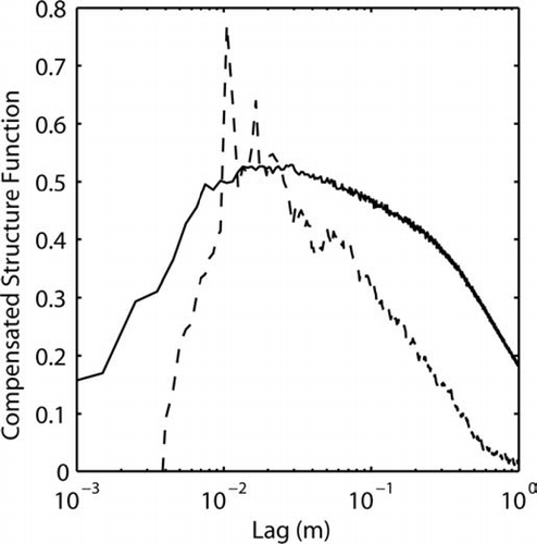
Regarding the suitability of measuring droplet rather than fluid speed, we recall the conclusions reached in Section 4.2 that for typical cloud conditions the droplet diameter must be below d ≈ 60 μ m. All droplets for the cloud data displayed in Figure 12 satisfy the condition d < 20 μ m so we can safely conclude that the measurements accurately reflect the fluid speed. In the laboratory flow (cf. Figure 13), similar considerations for droplet slip velocity lead to d < 20 μ m for s < 0.01 at a scale of 0.01 m. Droplets selected for use in calculating the results shown in Figure 13 satisfy the slightly more stringent condition d < 15 μ m. The excellent agreement between independent fluid-velocity measurements (i.e., from the sonic anemometer in the cloud and from the hotwire anemometer in the wind tunnel) and the droplet-velocity measurements suggests that the simple model for droplet-fluid coupling is reasonable.

5. SUMMARY AND CONCLUSIONS

Airborne measurement of the cloud drop size distribution utilizing the phase Doppler interferometry technique is advantageous compared to previous techniques for a number of reasons:

1.	Drop size determination is independent of the intensity of scattered light.
2.	Theoretical drop size precision is high, < 1 μ m, although what can be achieved under flight conditions has not been well-established.
3.	Only a single instrument calibration is necessary.
4.	Large dynamic range (more than 50:1) in size can be measured.
5.	Coincidence of two smaller drops can not be mistaken for the presence of one larger drop.
6.	The view volume (as a function of drop size) can be determined by combining the drop size and velocity measurements. This permits accurate calculation of drop concentration.

The performance of the Artium Flight PDI is documented. Comparisons between derived LWC from the F/PDI and the Gerber PVM-100A probe have shown generally good agreement within the uncertainties that have previously been estimated, but have also highlighted some differences between the measurements. Comparisons of drop number distributions between the F/PDI and FSSP-100 reveal a ∼ 5 μ m difference in sizing, and a ∼ 20 to 50% difference in spectral breadth (as measured by d ₉₀–d ₁₀). Even accounting for such a sizing bias, we find that the measured concentrations in five size bins between 7 and 42 μ m are correlated, but can differ by between 20% and a factor of two (or more), with the FSSP consistent yielding higher concentrations. In the smallest size bin from 2 to 7 μ m, the FSSP estimates drop concentrations about one order of magnitude higher, which speculate may be related to noise in the FSSP.

Measurement of drop velocity as a function of size utilizing the same instrument is shown to be sufficient for studying in-cloud turbulence, with suitable configuration of the instrument optical parameters. The velocities can be determined at a spatial resolution of ∼ 10 cm, which is the equivalent of 1 kHz sampling for a platform moving at 100 m s⁻¹. Velocity precision is on the order of 1 cm s⁻¹, again depending on the platform speed and optical configuration. Equation (9) highlights the advantage of slow-flying platforms for turbulence measurements, given that drop velocity measurement precision varies directly with platform velocity. Comparison of velocity statistics derived from the PDI with fluid velocity measurements (both sonic and hot-wire anemometers) show agreement within measurement and data processing uncertainties in both laboratory and airborne applications.

Acknowledgments

This research was supported by NSF Physical Meteorology and Major Research Instrumentation (ATM-0320953, ATM-0535488, and ATM-0342651) and the ONR SBIR program. We thank Bob Bluth (CIRPAS) for his aid in funding the instrument development. We thank CIRPAS, Rick Flagan, and John Seinfeld (Caltech), and ONR for their efforts in making the MASE field mission a success. S. K. Cheah is acknowledged for his work in performing the Fluent calculations. We are grateful to Holger Siebert (Leibniz Institute for Tropospheric Research) for helpful discussions and for the ACTOS sonic anemometer data, and Zellman Warhaft for use of the Cornell wind tunnel for instrument testing. Jean-Louis Brenguier (Météo-France) is acknowledged for his helpful comments. Finally, we owe many thanks to Jim Smith (NCAR) for the discussions that initiated this project many years ago as well as those since then.

Notes

¹Note that PDI-based instruments are sometimes referred to with the name Phase Doppler Particle Analyzer, or PDPA.

REFERENCES

- Albrecht , H.-E. , Damaschke , N. , Borys , M. and Tropea , C. 2003 . Laser Doppler and Phase Doppler Measurement Techniques , 750 Springer Verlag .
- Andrejczuk , M. , Grabowski , W. W. , Malinowski , S. P. and Smolarkiewicz , P. K. 2006 . Numerical Simulation of Cloud-Clear Air Interfacial Mixing: Effects on Cloud Microphysics . J. Atmos. Sci. , 63 : 3204 – 3225 .
- De Araujo Coelho , A. , Brenguier , J.-L. and Perrin , T. 2005 . Droplet Spectra Measurements with the FSSP-100. Part 1: Coincidence Effects . J. Atmos. Ocean. Tech. , 22 : 1756 – 1761 .
- Bachalo , W. D. 1980 . A Method for Measuring the Size and Velocity of Spheres By Dual Beam Light Scatter Interferometry . Applied Optics , 19 ( 3 )
- Bachalo , W. D. 1994 . The Phase Doppler Method: Analysis, Performance Evaluations, and Applications . Part. Part. Syst. Charact. , 11 : 73 – 83 .
- Bachalo , W. D. Measurement Techniques for Turbulent Two-Phase Flow Research . Presented International Symposium on Multiphase Fluid, Non-Newtonian Fluid and Physicochemical Fluid Flows (ISMNP) . October 7–9 1997 , Beijing, China.
- Bachalo , W. D. and Houser , M. J. 1984 . Phase Doppler Spray Analyzer for Simultaneous Measurements of Drop Size and Velocity Distributions . Optical Engineering , 23 ( 5 )
- Bachalo , W. D. and Sankar , S. V. 1996 . “ Phase Doppler Particle Analyzer ” . In The Handbook of Fluid Dynamics , Edited by: Johnson , R. W. 37.1 – 37.19 . Idaho Falls : CRC .
- Benedict , L. H. , Nobach , H. and Tropea , C. 2000 . Estimation of Turbulent Velocity Spectra From Laser Doppler Data . Meas. Sci. Technol , 11 : 1089 – 1104 .
- Brenguier , J.-L. , Bourrianne , T. , De Araujo Coelho , A. , Isbert , J. , Peytavi , R. , Trevarin , D. and Weschler , P. 1998 . Improvements of Droplet Size Distribution Measurements with the Fast-FSSP (Forward Scattering Spectrometer Probe) . J. Atmos. Ocean. Tech. , 15 : 1077 – 1090 .
- Cooper , W. A. 1988 . Effects of Coincidence on Measurements with a Forward Scattering Spectrometer Probe . J. Atmos. Ocean. Tech. , 5 : 823 – 832 .
- Davidson , P. A. 2004 . Turbulence: An Introduction for Scientists and Engineers , 678 New York : Oxford University Press .
- Davis , E. J. and Schweiger , G. 2002 . The Airborne Microparticle: Its Physics, Chemistry, Optics and Transport Phenomena , 833 Heidelberg : Springer Verlag . Sec. 4.7.6
- Gerber , H. 1991 . Direct Measurement of Suspended Particulate Volume Concentration and Far-Infrared Extinction Coefficient with a Laser Diffraction Instrument . Appl. Opt. , 30 : 4824 – 4831 .
- Gerber , H. , Arends , B. G. and Ackerman , A. S. 1994 . New Microphysics Sensor for Aircraft Use . Atmos. Res. , 31 : 235 – 252 .
- Gerber , H. , Frick , G. and Rodi , A. R. 1999 . Ground-Based FSSP and PVM Measurements of Liquid Water Content . J. Atmos. Ocean. Tech. , 16 : 1143 – 1149 .
- Glantz , P. , Noone , K. J. and Osborne , S. R. 2003 . Comparisons of Airborne CVI and FSSP Measurements of Cloud Droplet Number Concentrations in Marine Stratocumulus Clouds . J. Atmos. Ocean. Tech. , 20 : 133 – 142 .
- Kundu , P. K. and Cohen , I. M. 2004 . Fluid Mechanics, , Third Edition , San Diego, CA : Elsevier Academic Press .
- Lawson , R. P. , O'Connor , D. , Amarzly , P. , Weaver , K. , Baker , B. , Mo , Q. and Jonsson , H . 2006 . The 2D-S (Stereo) Probe: Design and Preliminary Tests of a New Airborne, High-Speed, High-Resolution Particle Imaging Probe . J. Atmos. Ocean. Tech. , 23 : 1462 – 1477 .
- Lu , M.-L. , Conant , W. C. , Jonsson , H. H. , Varutbangkul , V. , Flagan , R. C. and Seinfeld , J. H. 2007 . The Marine Stratus/Stratocumulus Experiment (MASE): Aerosol-Cloud Relationships in Marine Stratocumulus . J. Geophys. Res. , 112 D10209, Doi: 10.1029/2006JD007985
- Pruppacher , H. R. and Klett , J. D. 1997 . Microphysics of Clouds and Precipitation , Dordrecht, , The Netherlands : Reidel .
- Sankar , S. V. and Bachalo , W. D. 1991 . Response Characteristics of the Phase Doppler Particle Analyzer for Sizing Spherical Particles Larger Than the Light Wavelength . Applied Optics , 30 ( 12 )
- Saw , E. W. , Shaw , R. A. , Ayyalasomayajula , S. , Chuang , P. Y. and Gylfason , A. 2007 . Inertial Clustering of Particles in High-Reynolds-Number Turbulence . Physical Review Letters , in Review
- Schmidt , S. , Lehmann , K. and Wendisch , M. 2004 . Minimizing Instrumental Broadening of the Drop Size Distribution with the M-Fast-FSSP . J. Atmos. Ocean. Tech. , 21 : 1855 – 1867 .
- Schneider , J. M. and Hendricks , C. D. 1964 . Source of Uniform-Sized Liquid Droplets . Rev. Sci. Instru. , 35 : 1349 – 1350 .
- Shaw , R. A. 2003 . Particle-Turbulence Interactions in Atmospheric Clouds . Ann. Rev. Fluid Mech. , 35 : 183 – 227 .
- Siebert , H. and Teichmann , U. 2000 . Behaviour of an Ultrasonic Anemometer Under Cloudy Conditions . Bound.-Lay. Meteor , 94 : 165 – 169 .
- Siebert , H. , Lehmann , K. and Wendisch , M. 2006a . Observations of Small-Scale Turbulence and Energy Dissipation Rates in the Cloud Boundary Layer . J. Atmos. Sci. , 63 : 1451 – 1466 .
- Siebert , H. , Franke , H. , Lehmann , K. , Maser , R. , Saw , E. W. , Schell , D. , Shaw , R. A. and Wendisch , M. 2006 . Probing Fine-Scale Dynamics and Microphysics of Clouds with Helicopter-Borne Measurements . Bull. Amer. Meteor. Soc. , 87 : 1727 – 1738 .
- Siebert , H. , Lehmann , K. and Shaw , R. A. 2007 . on the Use of Hot-Wire Anemometers for Turbulence Measurements in Clouds . J. Atmos. Oceanic Technol , 24 : 980 – 993 .
- Vaillancourt , P. A. and Yau , M. K. 2000 . Review of Particle-Turbulence Interactions and Consequences for Cloud Physics . Bull. Amer. Meteor. Soc. , 81 : 285 – 298 .
- Wendisch , M. , Keil , A. and Korolev , A. V. 1996 . FSSP Characterization with Monodisperse Water Droplets . J. Atmos. Ocean. Tech. , 13 : 1152 – 1165 .
- Wendisch , M. , Garrett , T. J. and Strapp , J. W. 2002 . Wind Tunnel Tests of the Airborne PVM-100A Response to Large Droplets . J. Atmos. Ocean. Tech. , 19 : 1577 – 1584 .