Constraining Particle Evolution from Wall Losses, Coagulation, and Condensation-Evaporation in Smog-Chamber Experiments: Optimal Estimation Based on Size Distribution Measurements

Abstract

A goal of secondary organic aerosol (SOA) experiments performed in smog chambers is to determine the condensation of SOA onto suspended particles. Complicating the calculation of the condensation rate are uncertainties in particle wall-loss rates. Wall-loss rates generally depend on particle size, turbulence in the bag, the size and shape of the bag, and particle charge. In analyzing smog-chamber data, some or all of the following assumptions are commonly made regarding the first-order wall-loss rate constant: (a) that it is constant during an experiment; (b) that it is constant between experiments; and (c) that it is not a strong function of particle size for the relatively narrow size distributions in smog chamber experiments. Each of these assumptions may not be justified in some circumstances. We present the development and evaluation of the Aerosol Parameter Estimation (APE) model. APE is an inverse model that solves the aerosol general dynamic equation to determine best estimates for the size-dependent condensation rate and size-dependent wall-loss rate as a function of time. Size distribution measurements from a Scanning Mobility Particle Sizer (SMPS) provide time boundary conditions that constrain the general dynamic equation. The APE model is tested using data from a smog chamber experiment with dry ammonium sulfate particles in which no condensation occurred. Finally, we assess the variability in predicted SOA production between different wall-loss correction methods for relatively-fast-chemistry limonene-ozonolysis experiments and relatively-slow-chemistry toluene-oxidation experiments. In the fast limonene experiments, wall-loss correction methods agree within 10% for SOA production, and in the slow toluene experiments, wall-loss correction methods disagree up to a factor of 2.

1. INTRODUCTION

Smog chambers are valuable tools for performing atmospheric chemistry experiments in a controlled environment. One significant class of experiments involves measuring particle growth (or evaporation) as a result of chemistry: these include SOA formation experiments and particle aging experiments. These experiments rely on measurements of particle mass (volume) changes. A major complication is that particles are lost to the walls during an experiment (Crump and Seinfeld 1981; McMurry and Rader 1985). These losses must be accounted for to determine the aerosol yields from oxidation of SOA precursor gases (Pathak et al. 2007; Odum et al. 1996; Donahue et al. 2005). Underestimating the wall loss will lead to an underprediction of the aerosol yield and vice-versa.

Wall-loss corrections are relatively small when chemistry is rapid and wall losses are relatively slow. However, any experiment where wall-loss greatly affects the total suspended mass of particles during the period of condensation demands a careful treatment of the wall losses; without this, potential errors are large. In addition, the wall-loss rate depends on particle size, the geometry of the bag, the turbulence and electric field within the chamber and the charge distribution on the particles (Crump and Seinfeld 1981; McMurry and Rader 1985). For uncharged particles in uncharged chambers, the size dependence of the wall-loss rate is similar to that for dry deposition of particles calculated from the resistance in series method (Seinfeld and Pandis 2006). Ultrafine particles (diameter < 100 nm) will diffuse through the quasi-laminar layer near the chamber walls. Larger particles (diameter > 500 nm) will gravitationally settle to the bottom of the chamber (inertial impaction may also impact larger particles in chambers with large turbulence). A minimum wall-loss rate occurs between these diameters. Turbulent mixing within the chamber increases wall-loss rates across all sizes when diffusion is the dominant removal mechanism (Crump and Seinfeld 1981). Particle loss to walls is also enhanced by charges on the particles and the walls of the Teflon chamber, greatly complicating the dependence of size on wall loss (McMurry and Rader 1985; McMurry and Grosjean 1985). The size-dependent wall-loss rate as a function of size for particles with zero through three charges in a sample chamber is shown in Figure 1 (rates found using theory of McMurry and Rader (1985)). The modeled spherical chamber has a radius of 1 m, a turbulence rate, k _e , of 1 s^{− 1} and a mean electric-field magnitude of 50 volts cm^{− 1}. For all particle charges, there is a minimum in the wall-loss rate between 500 and 1000 nm, with smaller particles being lost more efficiently due to larger Brownian diffusion rates and charge to mass ratios. The effect of charge on wall loss in actual experiments is difficult to quantify because the particle charge distribution as a function of size is generally not known during smog chamber experiments.

FIG. 1 Particle-wall loss rates as a function of size for particles with 0 through 3 net charges (positive or negative) for a spherical chamber with a radius of 1 m and a turbulence factor, k _e , of 1 s^{− 1} and a mean electric field magnitude of 50 volts cm^{− 1} (solid lines). Also shown is the time evolution of the net particle wall-loss rate (particle wall-loss rate summed over all charges) in the chamber when the particles initially have a Boltzmann charge distribution (dashed lines).

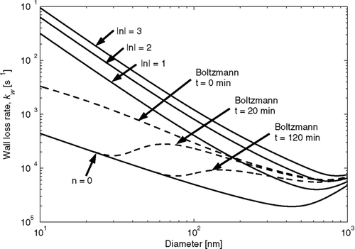
The dependence of wall loss on smog-chamber turbulence, geometry and particle/wall charge means that the size-dependent wall-loss rates will, in general, vary within and between experiments. In all smog chambers the flow of air in or out of the chamber can modify the turbulence in the bag. In chambers using a Teflon bag, forced airflow around the bag, such as for temperature control, and the variation of bag volume within or between experiments will change the geometry of the bag, the turbulence inside the bag, and subsequently the wall-loss rate. McMurry and Rader (1985) showed that the particle charge distribution can evolve during experiments, with charged particles being removed from chambers more quickly than uncharged particles. In the absence of particle charging mechanisms in the chamber, this will cause a reduction in the wall-loss rate over time at particle sizes where electrostatic forces dominate the wall-loss removal. This is illustrated in Figure 1 where we have plotted the time evolution of the net size-dependent wall-loss rate (including all particle charges) when the particles initially have a Boltzmann charge distribution (rates found using theory of McMurry and Rader (1985)). It is assumed that there is no charging mechanism within the chamber (e.g., cosmic rays or Rn²²² decay), charge is not redistributed from particle coagulation, and that charge is lost when a charged particle is removed by the wall. Initially the net size-dependent wall-loss rate is enhanced above the uncharged rate for all sizes. Within 20 minutes, nearly all of the charged particles smaller than 30 nm have been removed creating a minimum around 30 nm and a maximum near 65 nm. After 2 h, loss of charged ultrafine particles has shifted the minimum to 75 nm and the maximum to about 150 nm. Various methods of particle generation (e.g., atomization, nucleation, combustion) may result in particles with different initial charge distributions (Tsai et al. 2005; Forsyth et al. 1998) further complicating the effects of charging on wall loss.

Previous SOA-yield experiments have used a number of methods for accounting for particle losses to walls. One approach (Ng et al. 2007) involves measuring the size-dependent wall-loss rate of dry inert ammonium sulfate particles that undergo no condensation/evaporation during the experiment. If the number concentration of particles is low enough, the effect of coagulation is small and wall loss is the only process affecting the particle size distribution. This allows direct measurement the size-dependent wall-loss rate. This rate is subsequently used to correct for size-dependent wall loss in other experiments where the size-dependent wall-loss rate is impossible to measure. A key assumption is that the size-dependent wall-loss rate does not change during or between experiments. These wall-loss “calibrations” are repeated periodically. A second approach (Pathak et al. 2007) involves calculating the total-mass wall-loss rate constant in the chamber either before SOA condensation has started or after it is complete and then applying this rate to the entire experiment. This method assumes that the total-mass wall-loss rate does not change during the experiment. An advantage of this method is that day-to-day variations in the wall-loss rate are accounted for and the mass wall-loss rate is being quantified directly; however, this method loses accuracy if the total-mass wall-loss rate changes throughout the experiment. A third approach (Carter et al. 2005) involves determining the average number-loss rate of particles throughout the experiment. If the particle concentration is low, coagulation is not important and the number-loss rate is directly measured, if it is high, the total-number wall-loss rate is found by correcting the measurements for coagulation. This approach assumes that the wall-loss rate is not size dependent for the sizes of particles in the experiment, so that the total-number wall-loss rate is equal to the total-mass wall-loss rate. An advantage of this method is that day-to-day wall-loss variations are accounted for and the wall-loss rate is quantified throughout the condensation portion of the experiment; however, results may be incorrect if the wall-loss rate is strongly size dependent across the sizes of particles in the bag. A fourth method (Hildebrandt et al. 2008) is applicable for SOA production experiments where sulfate seeds are used and Aerosol Mass Spectrometer (AMS) data is taken. From the AMS, the time-dependent organic and sulfate concentrations are known throughout the experiment. Because there is no condensation/evaporation of sulfate during the experiment, the decay of this material provides a direct measure of the wall loss. The wall-loss rate, and subsequently the production rate of SOA, may be inferred from this information.

An alternative method for determining uncertain aerosol physics parameters in smog chamber experiments was suggested by Verheggen and Mozurkewich (2006). They use successive aerosol size-distribution measurements to estimate uncertain parameters in the aerosol general dynamic equation (Seinfeld and Pandis 2006). The wall loss in the Verheggen and Mozurkewich (2006) model follows the turbulent diffusion and gravitational settling model of Crump and Seinfeld (1981) and has one uncertain parameter that physically represents the amount of turbulence in the bag. This approach ignores the potential effect of charged particles on wall loss, and once the wall-loss rate was characterized in one experiment it is treated as known in other experiments (i.e., wall loss is no longer an uncertain parameter). Using a technique similar to that proposed by Verheggen and Mozurkewich (2006), we have developed the Aerosol Parameter Estimation (APE) model that uses size distribution measurements to estimate uncertain parameters in the aerosol general dynamic equation. However, where the model of Verheggen and Mozurkewich (2006) was tailored to determine changing nucleation and condensation rates, the APE model was customized to determine variable condensation and wall-loss rates.

The APE model is based on the following concept: coagulation, wall loss, and condensation/evaporation all influence the suspended-particle size distribution, but each influences number and mass differently. Coagulation changes number but not mass, wall loss changes number and mass, and condensation changes mass but not number. The objective of SOA formation experiments is to determine condensation/evaporation. Coagulation and wall loss are thus both interferences. While the coagulation rate can be quantified, many factors controlling wall loss are unknown. However, almost all SOA experiments contain measurements of the particle size distribution as a function of time throughout an experiment. Any interpretation of smog-chamber data must at least be consistent with these size-distribution constraints. The APE model uses the theory describing the coupled coagulation/wall-loss/condensation/evaporation system and the constraints of the size-distribution measurements to determine best estimates for the uncertain parameters (e.g., the condensation/evaporation and wall-loss rates). The time-dependent estimates of these parameters can be derived for each experiment without assumptions about the size-dependent wall-loss rate from prior experiments.

The goals of this article are as follows:

1. Develop the Aerosol Parameter Estimation (APE) model.

2. Test the ability of the APE model to predict known condensation/evaporation and size-dependent wall-loss rates.

3. Evaluate the uncertainty in estimates of SOA production due to the uncertainty in wall-loss rate by comparing various wall-loss correction methods.

Section 2 will describe the theory involved with the Aerosol Parameter Estimation (APE) model. The model is tested using a controlled ammonium sulfate aerosol experiment in section 3. In section 4, we will compare estimates of SOA produced by using the APE model along with three other wall-loss correction methods for limonene and toluene oxidation and discuss the uncertainty in the SOA due to uncertainty in the wall loss. Finally, the conclusions are given in section 5.

2. THE AEROSOL PARAMETER ESTIMATION (APE) MODEL

The aerosol general dynamic equation (GDE) (Seinfeld and Pandis 2006) predicts the evolution of the aerosol size distribution with time; however in smog chamber experiments, the aerosol size distribution is, in general, measured every few minutes by a Scanning Mobility Particle Sizer (SMPS) or a similar instrument. The predictions of the aerosol GDE are, therefore, constrained by these measurements. The goal of the Aerosol Parameter Estimation (APE) model is to fit the values of the unknown parameters in the GDE to obtain a best fit of the GDE predicted size distribution to the measured size distribution.

In this section we begin by describing the GDE along with what we do and do not know about the various processes in the GDE (e.g., coagulation, condensation, wall loss) during smog-chamber experiments and discuss the assumptions that are made regarding these processes in the APE model. We will then show how the APE model uses the time series of aerosol size distribution measurements to determine best estimates for the unknown values in the GDE (e.g., the condensation rate).

2.1. The Aerosol General Dynamic Equation

In a batch smog chamber experiment, the processes that can affect the aerosol size distribution are nucleation, coagulation, condensation/evaporation, and wall loss. In this article we will focus on experiments during which nucleation does not occur. The aerosol general dynamic equation may then take the following form:

In these equations, D _p is the diameter of the particle and N is the cumulative number distribution function (number of particles smaller than D _p ). Equation (1) represents the change in the aerosol number size distribution due to for coagulation, condensation/evaporation and wall loss. In the next subsections, we will describe what we do and do not know about these three processes during smog chamber experiments.

2.1.1. Coagulation

The change in the number distribution due to coagulation is (Seinfeld and Pandis 2006):

where K(D _p1, D _p2) is the coagulation kernel for collisions between particles of diameter D _p1 and diameter D _p2 (Seinfeld and Pandis 2006). The first term on the right accounts for two particles coagulating and forming a new particle with diameter D _p . The second term on the right accounts for particles with size D _p coagulating with all other particles.

If the aerosol size distribution is measured using a Scanning Mobility Particle Sizer (SMPS) or similar instruments then the coagulation kernel, K, may be calculated from theory (Seinfeld and Pandis 2006). Thus, the effects of coagulation on the size distribution can be well constrained. There are no uncertain parameters in the APE model associated with coagulation.

2.1.2. Condensation/Evaporation

The change in the number distribution due to condensation/evaporation is (Seinfeld and Pandis 2006):

In this equation, I(D _p ) is the rate of change of aerosol diameter depends on mass transfer rates (Seinfeld and Pandis 2006):

where D _i is the gas-phase diffusivity of the condensing species, M _i is the molecular weight of the condensing species, ρ _p is the density of the particle, R is the gas constant, T is the temperature, f is a correction for non-continuum particle effects, Kn is the Knudson number, α is the mass accommodation coefficient, p _i is the partial pressure of the condensing species in the bulk gas phase and p _eq,i is the vapor pressure of the condensing species in equilibrium with the particle.

A challenge is that many of the parameters in Equation (5) are unknown are unknown and cannot be measured in a smog-chamber experiment. Therefore, we lump many of these unknown parameters together into a single parameter, F _c .

We assume that particle composition is size-independent and surface tension effects are negligible, so F _c is itself size-independent. With the exception of the accommodation coefficient, α, all of the variables in Equation (5) that we are unable to measure directly in smog chamber experiments (D _i , M _i , ρ _p , p _i , p _eq,i ) are included in F _c . If we assume that α equals 1, F _c becomes the only unknown variable in the description of condensation in the GDE. If α is not equal to 1, this error may be largely compensated for by a lower value of F _c . Additional error may also occur from this treatment if the net condensation/evaporation of the vapors depends on particle mass rather than surface area as would be true for a vapor partitioning into the bulk of the particle. The APE model thus determines the best estimate of F _c to match the measured size distributions.

2.1.3. Wall Loss

The loss of particles to the walls of the chamber is a first-order loss process that depends on the size of the particles:

where k _w is the first-order wall-loss rate constant. k _w is not only size-dependent, it also depends on the size and shape of the chamber, the turbulence in the bag, the number of charges on the particle and the electric field in the bag.

A detailed treatment of how to determine k _w in the absence of electrostatic forces is given in Crump and Seinfeld (1981) and the determination of k _w in the presence of electrostatic forces is given in McMurry and Rader (1985). Unfortunately, these methods require knowledge of the turbulent kinetic energy in the chamber, the size-dependent charge distribution on the particles and the average magnitude of the electric field in the chamber. All of these parameters are difficult to quantify, and no attempt is typically made to do so in smog chamber experiments. Because we cannot predict k _w directly using these techniques, the APE model determines k _w by fitting various functional forms of the size-dependent wall-loss rate to the time- and size-dependent aerosol data from a smog chamber experiment. Here we describe the three functional forms of the size dependent wall-loss rate that depend on one or two unknown parameters that will be used in the APE model.

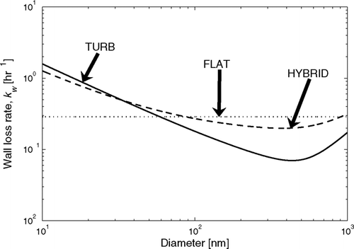
The first and simplest functional form of wall-loss size dependence used in the APE model is that wall loss is independent of size over the size distribution at any given time. This functional form makes k _w in Equation (7) size independent, but allows it to vary during the experiment. Experiments with large changes in the size distribution will see changes in the wall-loss rate over the course of the experiment. This form involves one unknown parameter, the value of k _w . This case will be referred to as “FLAT” throughout the article. An example of the FLAT case is shown as the dotted line in Figure 2.

FIG. 2 Example of the modeled wall loss rates using the FLAT (1 free parameter: k _w = 8 × 10^{− 5} s^{− 1}), TURB (1 free parameter: k _e = 1 s^{− 1}), and HYBRID (2 free parameters: k _w0 = 4 × 10^{− 5} s^{− 1}, k _e = 0.5 s^{− 1}) assumptions.

For the second functional form of wall-loss size dependence we assume that our chamber is spherical and that the charging of particles is negligible. The size-dependent wall loss will then follow the theory of Crump and Seinfeld (1981):

where k _e (units time^{− 1}) is a function of the turbulent kinetic energy in the chamber, D is the Brownian diffusivity of the particle of size D _p , R is the radius of the bag, and v _s is the gravitational settling velocity of the particle. D ₁ is the Debye function (Abramowitz and Stegun 1965):

All values in this equation are known or may be directly measured except for k _e . Similar to FLAT, there is one unknown parameter, in this case, k _e . Because the unknown parameter in this functional form is proportional to the turbulence in the bag, this case will be referred to as “TURB” throughout the article. An example of the TURB case is shown as the solid line in Figure 2.

The third and final functional form is a rough attempt to account for the possible effect of electrostatic forces on wall loss without greatly complicating the functional form of the wall-loss size dependence. McMurry and Rader (1985) and our Figure 1 showed that because the smallest charged particles get lost to the walls very quickly and larger particles have a larger surface area, particles with D _p > 100 nm tend to be more charged than small particles. This means that the wall-loss rate for the particles D _p > 100 nm will be enhanced relative to the TURB case (Boltzmann lines in Figure 1). To account for this we use the empirical wall-loss size dependence:

This is just a linear combination of the functional forms of the FLAT and TURB assumptions (Equations [7] and [8]). In this case there are two unknown parameters, k _w0 and k _e . Because it is a hybrid of the previous two cases, this case will be referred to as “HYBRID” throughout the article. An example of the HYBRID case is shown as the solid line in Figure 2. Note that HYBRID results in a weaker size dependence than the TURB approach.

Between condensation/evaporation and wall loss, the APE model must solve for 2 unknown parameters (in the FLAT and TURB cases) or 3 unknown parameters (in the HYBRID case).

2.2. Solving the APE Model

In order to solve numerically the GDE between SMPS scans, we discretize the aerosol number size distribution into the size sections of the SMPS (usually 100–110 logarithmically spaced size sections between 10 nm and 500–800 nm). The number size distribution, n, as shown in Equation (2), is assumed to be constant within each size section. The size distribution is initialized with the measurement an SMPS scan. The discretized GDE is solved numerically using the Dormand-Prince pair 4th and 5th order Runge-Kutta method to provide an estimate of the aerosol size distribution at the time of the next SMPS scan. The finite difference approximation of the coagulation term is the same as in Verheggen and Mozurkewich (2006).

In order to find the best-estimate values of the unknown condensation/evaporation and wall-loss parameters, we use non-linear least-squares fitting optimization of the unknown parameters in the GDE. The GDE is first solved as described in the previous paragraph while using initial guesses for the unknown parameters. The procedure is then repeated with new guesses for the unknown parameters until the GDE predicted size distribution and the measured size distribution agree using the criteria described below.

To smooth variability between SMPS size bins, the fit of the predicted size distributions to the observed size distributions are quantified by comparing various diameter moments of the aerosol size distribution. The total of a given diameter moment of the size distribution is found using the following equation:

where i refers to the ith diameter moment of the distribution and M _i is the total ith diameter moment. The 0th and 1st diameter moments have physical basis in that they are the total number of particles and the total diameter of all the particles combined. The 2nd diameter moment is proportional to the total aerosol surface area and the 3rd diameter moment is proportional to the total volume of particles. The optimum fit is determined by minimizing X ²:

In this equation i(a) is the set of diameter moments (−1, −0.5, 0, 0.5, 1, 1.5, 2, 2.5, 3). The subscript p indicates the predicted moment and o denotes the observed moment. Matching a wide range of total diameter moments helps fit the predicted distribution to the observed distribution at both small and large sizes. The range of moments was chosen to help fit accurately both the total number (0th moment) and the total volume (proportional to the 3rd moment) while simultaneously predicting the shape of the distribution. It is possible to apply a least-squares fit where the fitted data are the number of particles in each SMPS size section; however, increased relative error in size sections with lower particle counts makes this difficult.

3. MODEL EVALUATION

We test the APE model with data from a smog-chamber experiment where the condensation/evaporation and size-dependent wall-loss rates are known. In this ideal test case, the smog chamber is initially filled with dry ammonium sulfate aerosol and these particles coagulate and are lost to the walls. No condensation/evaporation occurs in this experiment. For the APE model to analyze the experiment successfully, it must predict that little or no condensation/evaporation occurred throughout the experiment and also predict the size dependence of the wall-loss rate. Because the condensation/evaporation rate is unconstrained in the APE model, correctly predicting zero condensation/evaporation is as rigorous a test as predicting correctly a non-zero value. The three wall-loss functional forms for the APE model described above are individually tested in this section to see how well they reproduce the correct condensation/evaporation and wall loss.

This ammonium sulfate experiment was performed in the Carnegie Mellon University smog chamber (CMU-SC). The chamber consists of a Teflon bag with a volume that varies between 10–12 m³ contained in a temperature controlled room. The bag has a shape somewhere between a sphere and a cube, and for the calculations of the wall-loss rate in the TURB and HYBRID cases, we assume that the bag is spherical with a radius of 1.4 m. Further details of the chamber and its instrumentation are included in previous work (Huff-Hartz et al. 2005; Stanier et al. 2007; Presto et al. 2005).

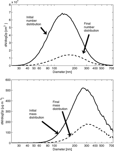
The ammonium sulfate particles are formed by atomization (TSI model 3076) and dried using diffusion driers to remove water and crystallize the particles. A Boltzmann charge distribution is applied to the particles by passing them through a neutralizer (Kr-85) prior to entering the smog chamber. Prior to the experiment, the CMU-SC was flushed with clean, particle free air overnight. The relative humidity of the smog chamber was between 5 and 10% throughout the experiment. Particle concentrations in the chamber were monitored with an SMPS (TSI, model 3080). The time for one complete SMPS scan was 210 seconds. The smog chamber analysis using the APE model began after the addition of particles ceased, and the initial number concentration was 4 × 10⁴ cm^{− 3}. Figure 3 shows the initial and final (4 h later) number and mass size distributions for this ammonium sulfate experiment.

FIG. 3 Initial and final (4 h later) number and mass size distributions during the ammonium sulfate experiment.

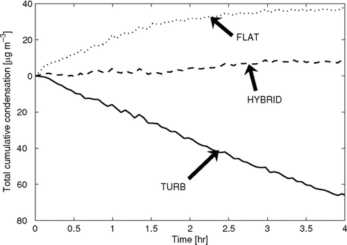
The ammonium sulfate particles in the chamber should be dry when entering the chamber, and in the absence of condensable gases, the condensation/evaporation onto the particles is zero. Figure 4 shows the estimated total cumulative mass condensed onto the suspended particles for the three wall-loss functional forms as predicted by the APE model. For reference to the relative magnitude of this condensation, the initial total mass of particles was 280 μ g m^{− 3} and the total suspended mass of particles at the end of the experiment was 100 μ g m^{− 3}. The HYBRID case performs the best, predicting less than 7 μ g m^{− 3} of condensation during the experiment. The FLAT case incorrectly predicted almost 40 μ g m^{− 3} of condensation though the first two hours of the experiment, eventually leveling off. An opposite, but equally incorrect, outcome occurred in the TURB case with about 60 μ g m^{− 3} of evaporation through the four hours of the experiment. We expect that these absolute errors would scale with the amount of mass in the experiment and the relative errors are constant.

FIG. 4 The calculated total cumulative condensation onto the suspended particles as a function of time for the ammonium sulfate experiment. The predicted condensation depends on the wall-loss functional form. For reference, the initial mass concentration of particles in the chamber was 280 μ g m^{− 3}.

Figure 5 compares the time-averaged size-dependent wall-loss rates for the entire 4 h experiment for the three wall-loss functional forms in the APE model. Also included in Figure 5 is our best estimate for the time-averaged size-dependent wall-loss rate found by taking the time-averaged size-dependent number-loss rate of particles directly from the SMPS data and correcting for the number-loss from coagulation. This best estimate is labeled “No condensation” in Figure 5 and is likely very close to the actual size-dependent wall-loss rate. Please note that this best estimate is not found using the APE model, but found using the assumption that no condensation occurred. To estimate the uncertainty in the coagulation correction, we scaled the coagulation rates (for all particles sizes) up and down by 20% to determine the bounding lines above and below the “No condensation” line. Any potential uncertainty in the coagulation has only a small effect on our best estimate except for at the smallest sizes. The shape of this “No condensation” wall-loss curve shows a maximum wall-loss rate around 100 nm, with a gradual decrease with larger sizes and a sharper decreases with smaller sizes to what appears to be a minimum around 50 nm, similar to the “Boltzmann t = 20 min” and “Boltzmann t = 120 min” curves in Figure 1. Unfortunately, there were not enough particles smaller than 50 nm to determine if wall-loss rate increases with decreasing size for these nanoparticles. The resemblance of the “No condensation” curve in Figure 5 to the “Boltzmann t = 20 min” and “Boltzmann t = 120 min” curves in Figure 1 is logical because the particles in both of these cases are initialized with a Boltzmann charge distribution. Also shown are the initial and final mass median diameters of this experiment.

FIG. 5 Average wall loss rates as a function of diameter during the ammonium sulfate experiment for the three wall-loss functional forms and the time-averaged wall-loss rate calculated assuming that there was no condensation/evaporation during the experiment corrected for coagulation (No condensation). The uncertainty in the wall-loss rate due to uncertainty in the coagulation kernel is shown by the lines above and below the no condensation line. In these lines, the entire coagulation kernel was scaled up and down by 20%.

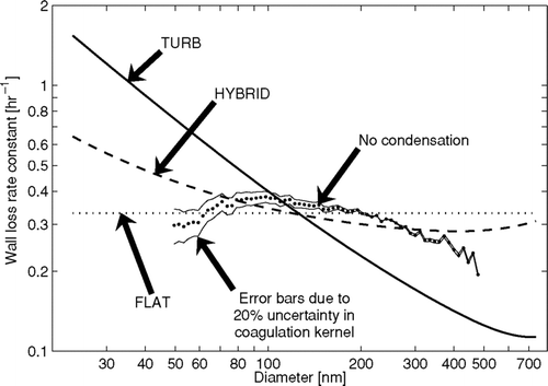
The reason for the incorrect prediction of condensation/evaporation by the FLAT and TURB cases can be understood by comparing the different estimates in Figure 5. The size-dependent wall-loss rate predicted in the FLAT case tends to remove large particles more quickly than the “No condensation” values. Therefore, the APE model uses condensation to compensate for the overestimate of the loss of larger particles that contain much of the mass in the chamber. This explains the net condensation predicted by the FLAT case in Figure 4. In experiments where the aerosol size distribution is narrow and is located at sizes where the wall-loss rate is not strongly size dependent, the FLAT case should perform better. The size-dependent wall-loss rate predicted in the TURB case tends to remove small particles too quickly and large particles too slowly compared to the observed values. Therefore, the APE model uses evaporation to allow the predicted size distribution to better match the measured size distribution. This is the reason for the net evaporation predicted by the TURB case in Figure 4. The HYBRID does not exactly reproduce the features of the observed size-dependent wall-loss rates; specifically, it does not reproduce the maximum wall-loss rate near 100 nm. However, the HYBRID case tends to have less error across the size distribution than the TURB and FLAT cases and hence correctly predicted close to zero condensation/evaporation. It is important to remember that while the HYBRID method did by far the best of the three wall-loss functional forms in this test, it was not perfect in predicting the size-dependent wall-loss rate and condensation/evaporation rate. We will, however, continue to use the HYBRID wall-loss functional form throughout the rest of the article. We will not use the FLAT and TURB forms because of their inability to determine zero condensation/evaporation in this controlled case.

4. UNCERTAINTY IN ESTIMATES OF SOA PRODUCTION DUE TO WALL-LOSS CORRECTIONS

In this section we investigate how uncertainties in the wall-loss rate influence estimates of SOA production by comparing results using three different wall-loss correction methods of SMPS data. We analyzed 9 SOA-production experiments that were performed in the CMU-SC: 5 experiments where limonene vapors reacted with ozone, which had condensation timescales much shorter than the wall-loss timescales, and 4 experiments where toluene vapors reacted with the hydroxyl radical, which had condensation timescales similar to the wall-loss timescales. Throughout this analysis, we assume that all semivolatile vapors condense onto suspended particles (not to the wall or particles already lost to the wall) (Weitkamp et al. 2007).

A total of three wall-loss correction methods will be tested. The first method is the extrapolation method described in Pathak et al. (2007) (EXTRAPOLATE). In this method we quantify the size-independent mass wall-loss rate after condensation has completed. The mass wall-loss rate is then extrapolated throughout the condensation portion of the experiment and the total amount of SOA condensed between each SMPS time step is found by determining the difference between the measured change in mass and the change in mass from total-mass wall-loss alone. The second method is the average number wall-loss method described in Carter et al. (2005) (NUMBER-AVG). Here we find the average total-number wall-loss rate corrected for coagulation throughout the entire experiment and assume that this total-number wall-loss rate is the same as the total-mass wall-loss rate. Similar to the EXTRAPOLATE method, the SOA produced between each SMPS time step is found by determining the difference between the measured change in mass and the change in mass from total-mass wall-loss alone. The third method is the HYBRID version of the APE model (APE-HYBRID) that was described above.

4.1. Limonene SOA

In each of the limonene experiments, the chamber is initially filled with ammonium sulfate aerosol seeds and ozone prior to the injection of limonene. The full procedure for these experiments is described in Pathak et al. (2007). Information about the limonene experiments, including mass-mean aerosol diameters and total suspended mass concentrations at the time of limonene injection and one hour later, for each of the five experiments is given in Table 1. For these limonene experiments the atomized particles were added to the chamber with no neutralization, so their initial charge distribution was likely larger than a Boltzmann distribution (Tsai et al. 2005; Forsyth et al. 1998). This may cause the wall-loss effects of charge to be quite strong, at least initially. In each experiment, the aerosol mass concentration 1 h after the limonene was injected is larger than the mass before, showing that condensation contributes more to the changing mass than wall loss.

TABLE 1 Limonene oxidation experiments

	Limonene conc.	Ozone conc.	Temp.	MMDi	MMD1	TSMi	TSM1
Exp.	[ppb]	[ppb]	[K]	[nm]	[nm]	[μ g m^− 3]	[μ g m^− 3]
1	20	500	288	170	224	77	147
2	20	500	313	176	208	54	85
3	5	500	288	184	215	54	70
4	10	500	313	179	216	44	78
5	2	500	288	175	208	37	42
MMDi = Mass median diameter of aerosol prior to chemistry/condensation.
MMD1 = Mass median diameter of aerosol after 1 h of chemistry/condensation.
TSMi = Total suspended mass concentration before chemistry/condensation.
TSM1 = Total suspended mass concentration after 1 h of chemistry/condensation.

Figure 6 shows the total-mass wall-loss rate as a function of time for the five limonene experiments as predicted by the EXTRAPOLATE, NUMBER-AVG and APE-HYBRID methods. Time zero corresponds to when limonene is injected into the chamber and the seed particles begin to grow through condensation. The APE-HYBRID method is the only method that resolves the wall loss as a function of time. In all of these experiments, the APE-HYBRID predicted total-mass wall-loss rate decreases rapidly within the first half hour after limonene injection. The fluctuations in the second half hour are smaller than this initial change. The initial drop in the total mass wall-loss rate may be due to the growth of the particles during this time period to sizes with slower wall-loss rates (Table 1). Another possible explanation for the decrease in wall-loss rate is that the number of charged particles in the chamber decreases because of the expedited loss of the charged particles to the wall relative to uncharged particles (McMurry and Rader 1985). The initial concentration of charged particles is high due to the atomization of seed particles without subsequent neutralization (Forsyth et al. 1998; Tsai et al. 2005).

FIG. 6 Total predicted mass wall-loss rate as a function of time in the limonene experiments using the EXTRAPOLATE, NUMBER-AVG, and APE-HYBRID methods. Note that the y-axes change for each experiment.

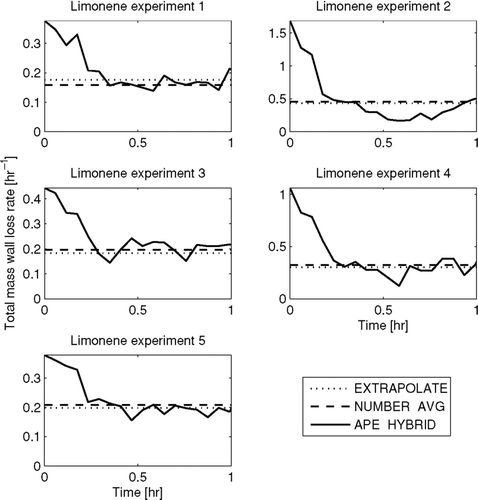
In all experiments, the EXTRAPOLATE and NUMBER-AVG methods predict similar total-mass wall-loss rates that are also similar to the final total-mass wall-loss rates predicted by the APE-HYBRID method. The agreement between the EXTRAPOLATE and the final APE-HYBRID total mass wall-loss rates is because the EXTRAPOLATE wall loss is fit to the actual total mass wall-loss rate at the end of the experiment, after the chemistry/condensation was complete. However, the cause of the agreement of the total-mass wall-loss rate from NUMBER-AVG with the APE-HYBRID method at the end of the hour is more difficult to determine. In the NUMBER-AVG method, the time-average total-number wall-loss rate of the experiment is found and wall loss is assumed to be size-independent such that the total-number wall-loss rate equals the total-mass wall-loss rate. If wall loss is in fact size independent and the APE-HYBRID method is predicting correctly the time-dependent total-mass wall-loss rate, the total-mass wall-loss rate predicted by the NUMBER-AVG method should be the average of the APE-HYBRID method. However, wall loss may not be size independent, and the APE-HYBRID model may not be predicting correctly the time-dependent total-mass wall-loss rate.

Figure 7 shows the predicted SOA condensation onto the particles in the chamber as a function of time for the three wall-loss correction methods used in Figure 6 as well as a case where wall loss is not corrected (UNCORRECTED). In Figure 7, proportional differences in the total mass condensed between these methods represent proportional differences in predicted SOA yield. It is clear from Figure 7 that nearly all of the condensation occurs during the first half hour.

FIG. 7 Total predicted condensation onto suspended particles as a function of time in the limonene-SOA experiments using the EXTRAPOLATE, NUMBER-AVG, and APE-HYBRID methods. Also shown is the total predicted condensation onto suspended particles if wall loss is not corrected for (UNCORRECTED). Note that the y-axes change for each experiment.

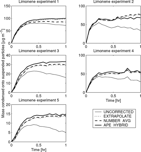
As would be expected from the UNCORRECTED case, the estimated mass of SOA decreases once chemistry and condensation has slowed due to not correcting for the mass lost to the walls. One hour into the experiment, when the condensation has stopped in all experiments, the UNCORRECTED case has deviated from the three loss-corrected cases by 20–60%. The three wall-loss correction methods predict SOA mass within 10% for all experiments. In all experiments except for experiment 2 the EXTRAPOLATE and NUMBER-AVG predict less mass condensed than APE-HYBRID. This general difference of the NUMBER-AVG and EXTRAPOLATE relative to APE-HYBRID is because the NUMBER-AVG and EXTRAPOLATE methods have lower total-mass wall-loss rates during the early portion of the condensation (Figure 6). We stress, however, that estimates from the APE-HYBRID method are not necessarily correct either. The APE-HYBRID model must predict accurately the time- and size-dependent wall-loss rate (unknown in these experiments) in order to properly predict the condensation.

Figure 7 shows that for these limonene experiments with rapid oxidation the uncertainty in the SOA yields vary by less than 10% among different wall-loss correction methods. The timescale for wall loss in the chamber in Figure 6 is of the order 1 to 5 h (with the longer timescales occurring after condensation has started), so the mass is being lost to the walls more slowly than the time it takes for condensation to occur. Also, the suspended mass is larger at the end of the hour than at the beginning, so the SOA condensation signal is strong compared to the uncertainty in the wall-loss rate.

4.2. Toluene SOA

Estimating the SOA production from slow reacting compounds such as toluene is more challenging because chemistry/condensation may occur with similar or longer timescales than wall loss. In these experiments, toluene vapor was oxidized by the hydroxyl radical. The chamber is initially filled with hydrogen peroxide vapor, ammonium sulfate aerosol seeds, toluene, and, in some experiments, NO. The oxidation begins (OH radicals are produced) when UV lights in the chamber are turned on. The full procedure is described in Hildebrandt et al. (2008).

Information about the toluene experiments, including mass-mean aerosol diameters and total suspended mass concentrations at the time the lights are turned on and three hours later, for each of the four experiments is given in Table 2. Unlike the limonene SOA experiments where condensation affected the aerosol mass more than wall loss in all cases, the final suspended mass (after 3 hours) in the toluene experiments was higher than the initial mass in 2 cases and lower in 2 cases, showing that wall loss plays a larger role in these experiments. Also unlike the limonene experiments, the ammonium sulfate seed particles in the toluene experiments are neutralized towards Boltzmann charge distribution before entering the bag.

TABLE 2 Toluene oxidation experiments

	Initial Toluene	Toluene cone.	NOx	Temp.	MMDi	MMD3	TSMi	TSM3
Exp.	conc. [ppb]	after 3 hours [ppb]	level	[K]	[nm]	[nm]	[μ g m^− 3]	[μ g m^− 3]
1	939	774	High	273	225	260	60	113
2	909	762	High	293	218	248	41	62
3	937	802	High	293	225	292	108	102
4	568	520	Low	294	204	221	60	31
MMDi = Mass median diameter of aerosol before chemistry/condensation.
MMD3 = Mass median diameter of aerosol after 3 h of chemistry/condensation.
TSMi = Total suspended mass concentration before chemistry/condensation.
TSM3 = Total suspended mass concentration after 3 h of chemistry/condensation.

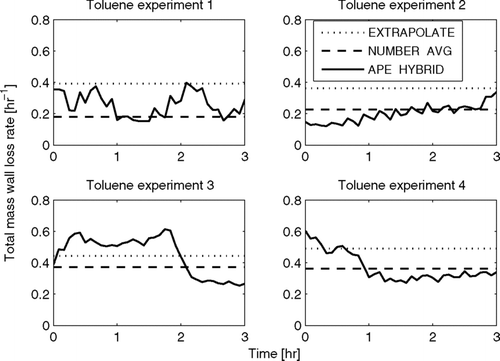
Figure 8 shows the estimated total-mass wall-loss rate as a function of time for the four toluene experiments as predicted by the EXTRAPOLATE, NUMBER-AVG, and APE-HYBRID methods. Time zero corresponds to when the lights are turned on, initializing oxidation, and the seed particles begin to grow through condensation. With the exception of experiment 4, the APE-HYBRID does not predict a decreasing trend in the total-mass wall-loss rate at the beginning of the experiment as it did with the limonene experiments. This may be because the initial loss of charged particles is smaller in the toluene experiments due to the neutralization of the seed particles. It may also be due to particle growth occurring more slowly so that other factors (e.g., changing bag shape, turbulence, or charge) may have a larger relative impact on changing the total-mass wall-loss rates. With the exception of experiment 2, the total-mass wall-loss rate from the EXTRAPOLATE method does not correspond to the APE-HYBRID at 3 h (as it did for 1 h in the limonene experiments). This is because the lights were turned off in these experiments at varying times that were, in general, much later than 3 h. The total-mass wall-loss rate for the EXTRAPOLATE method could not be quantified until after the lights were turned off. In all experiments except experiment 1, the NUMBER-AVG method tends to predict a value of the total-mass wall-loss rate similar to the average values of the APE-HYBRID method. In experiment 1, the NUMBER-AVG method predicts a total-mass wall-loss rate lower than the APE-HYBRID method average similar to the limonene experiments.

FIG. 8 Total predicted mass wall-loss rate as a function of time in the toluene SOA experiments using the EXTRAPOLATE, NUMBER-AVG, and APE-HYBRID methods.

Figure 9shows the total condensation onto the particles in the chamber as a function of time for the three wall-loss correction cases above. The UNCORRECTED method predicts negative values for SOA condensed at 3 h due to wall loss being larger than condensation in some experiments, so it is not shown here. It is clear from Figure 9 that the condensation occurs over hours, much longer than in the limonene ozonolysis (Figure 7).

FIG. 9 Total predicted condensation onto suspended particles as a function of time in the Toluene-SOA experiments using the EXTRAPOLATE, NUMBER-AVG, and APE-HYBRID methods. Note that the y-axes change for each experiment.

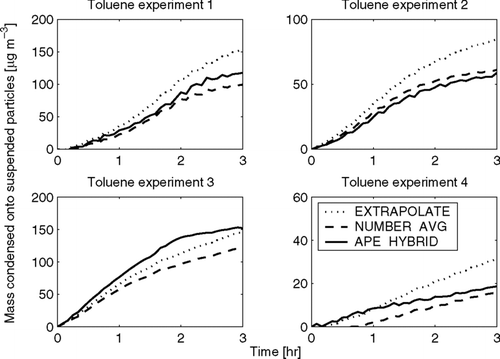
Unlike the limonene experiments, where the various wall-loss correction methods give SOA condensation predictions that were always within 10%, the three methods here diverge with 25–100% differences between the highest and lowest predictions in each experiment. In experiment 1, the EXTRAPOLATE prediction is about 50% higher than the NUMBER-AVG prediction, and the APE-HYBRID is in between. In experiment 2, the EXTRAPOLATE method is again the highest, about 40% higher than the other two predictions, which agree well. In experiment 3, the three predictions agree the closest (25%), and the APE-HYBRID predicts the highest amount of condensation. Experiment 4 has the highest disagreement, where the EXTRAPOLATE and NUMBER-AVG disagree by a factor of 2. The larger disagreement in experiment 4 may be because less toluene was oxidized in this experiment (Table 2); therefore, the mass change due to condensation is smaller relative to wall loss.

It is clear from the contrasting results between the limonene and toluene experiments that the uncertainty in wall-loss rate influences the predicted SOA condensation in these slower-chemistry toluene experiments much more significantly. Because the condensation occurred over a much longer timescale, a much larger fraction of the suspended mass was lost to the walls (∼ 60% of the initial aerosol was lost to the wall after 3 h) before the end of the experiment. In this case the uncertainty in the mass lost to the walls was similar in magnitude to the SOA condensed, so the SOA prediction is more uncertain. Finally, because the actual wall-loss and condensation rates are unknown, it is impossible for us to assess the individual accuracy of each of these correction techniques. We suggest their application in the same experiment can at least provide a good measure of the uncertainty introduced to the results because of wall-loss correction. It is unavoidable that wall-loss effects lead to larger uncertainties for experiments with longer timescales; the purpose here is to estimate bounds of these uncertainties.

5. CONCLUSIONS

We have developed the Aerosol Parameter Estimation (APE) model to decouple condensation and wall loss in smog chamber experiments, specifically to explore the uncertainty in estimates of SOA yield due to wall loss. The APE model is an inverse model that determines unknown condensation and wall-loss parameters by using aerosol size-distribution measurements to constrain these uncertain parameters in the aerosol general dynamic equation. Three functional forms of the wall-loss size dependence were tested in the APE model.

The ability of the APE model to predict the condensation/evaporation rate was tested in an experiment with inert dry ammonium sulfate aerosol. The HYBRID wall-loss functional form correctly predicted that very little condensation/evaporation occurred during the experiment, whereas the other two functional forms, the FLAT and TURB, both incorrectly predicted that condensation/evaporation occurred. The HYBRID form was chosen to be used for further evaluation.

Finally, the variability in predicted SOA production between different wall-loss correction methods was assessed for relatively fast chemistry limonene-ozonolysis experiments and relatively-slow-chemistry toluene-oxidation experiments. In the limonene experiments, where condensation affected the suspended aerosol mass more than wall loss, three wall-loss correction methods agreed within 10% for SOA production in all five experiments analyzed. In the toluene experiments, where wall loss and condensation affected the mass of suspended aerosol by similar magnitudes, three different wall-loss correction methods disagreed by up to a factor of 2. It is impossible for us to assess which of the wall-loss correction methods was most accurate during these analyses due to the true SOA production rate not being known. However, based on this comparison, we recommend, whenever possible, limiting SOA production experiments to those where the SOA condensation affects the suspended mass more greatly than wall loss (i.e., suspended mass increases during the experiment). For experiments where this constraint is difficult, we recommend using multiple techniques to correct for wall-loss effects to determine the affect of wall-loss uncertainty on the predicted amount of SOA produced.

J. R. Pierce was supported by the Environmental Protection Agency (EPA) through the Science to Achieve Results (STAR) Graduate Fellowship (91668201–0). G. J. Engelhart was supported by the National Science Foundation Graduate Research Fellowship and the Achievement Rewards for College Scientists. L. Hildebrandt was supported by the National Science Foundation Graduate Research Fellowship. The research was generally supported by the EPA STAR grant (R832162) and the Electric Power Research Institute (EPRI).

REFERENCES

- Abramowitz , M. and Stegun , I. A. 1965 . Handbook of Mathematical Functions Dover, New York.
- Carter , W. P. L. , Cocker , D. R. , Fitz , D. R. , Malkina , I. L. , Bumiller , K. , Sauer , C. G. , Pisano , J. T. , Bufalino , C. and Song , C. 2005 . A New Environmental Chamber for Evaluation of Gas-Phase Chemical Mechanisms and Secondary Aerosol Formation . Atmos. Environ. , 39 : 7768 – 7788 .
- Crump , J. G. and Seinfeld , J. H. 1981 . Turbulent Deposition and Gravitational Sedimentation of an Aerosol in a Vessel of Arbitrary Shape . J. Aerosol Sci. , 12 : 405 – 415 .
- Donahue , N. M. , Hartz , K. E. H. , Chuong , B. , Presto , A. A. , Stanier , C. O. , Rosenhorn , T. , Robinson , A. L. and Pandis , S. N. 2005 . Critical Factors Determining the Variation in SOA Yields From Terpene Ozonolysis: A Combined Experimental and Computational study . Faraday Discuss. , 130 : 295 – 309 .
- Forsyth , B. , Liu , B. Y. H. and Romay , F. J. 1998 . Particle Charge Distribution Measurement for Commonly Generated Laboratory Aerosols . Aerosol Sci. Technol. , 28 : 489 – 501 .
- Hildebrandt , L. , Donahue , N. M. and Pandis , S. N. 2008 . Formation and Properties of Secondary Organic Serosol from Toluene in preparation
- Huff-Hartz , K. E. , Rosenorn , T. , Ferchak , S. R. , Raymond , T. M. , Bilde , M. , Donahue , N. M. and Pandis , S. N. 2005 . Cloud Condensation Nuclei Activation of Monoterpene and Sesquiterpene Secondary Organic Aerosol . J. Geophys. Res. , 110 : D14208
- McMurry , P. H. and Grosjean , D. 1985 . Gas and Aerosol Wall Losses in Teflon Film Smog Chambers . Environ. Sci. Technol. , 19 : 1176 – 1182 .
- McMurry , P. H. and Rader , D. J. 1985 . Aerosol Wall Losses in Electrically Charged Chambers . Aerosol Sci. Technol. , 4 : 249 – 268 .
- Ng , N. L. , Kroll , J. H. , Chan , A. W. H. , Chhabra , P. S. , Flagan , R. C. and Seinfeld , J. H. 2007 . Secondary Organic Aerosol Formation from m-Xylene, Toluene, and Benzene . Atmos. Chem. Phys. , 7 : 3909 – 3922 .
- Odum , J. R. , Hoffmann , T. , Bowman , F. , Collins , D. , Flagan , R. C. and Seinfeld , J. H. 1996 . Gas/Particle Partitioning and Secondary Organic Aerosol Yields . Environ. Sci. Technol. , 30 : 2580 – 2585 .
- Pathak , R. K. , Stanier , C. O. , Donahue , N. M. and Pandis , S. N. 2007 . Ozonolysis of Alpha-Pinene at Atmospherically Relevant Concentrations: Temperature Dependence of Aerosol Mass Fractions (yields) . J. Geophys. Res. , 112 : D03201
- Presto , A. A. , Hartz , K. E. H. and Donahue , N. M. 2005 . Secondary Organic Aerosol Production from Terpene Ozonolysis. 1. Effect of UV Radiation . Environ. Sci. Technol. , 39 : 7036 – 7045 .
- Seinfeld , J. H. and Pandis , S. N. 2006 . Atmospheric Chemistry and Physics, , 2nd , New York : John Wiley and Sons .
- Stanier , C. O. , Pathak , R. K. and Pandis , S. N. 2007 . Measurements of the Volatility of Aerosols from Alpha-Piniene Ozonolysis . Environ. Sci. Technol. , 41 : 2756 – 2763 .
- Tsai , C. J. , Lin , J. S. , Deshpande , C. G. and Liu , L. C. 2005 . Electrostatic Charge Measurement and Charge Neutralization of Fine Aerosol Particles During the Generation Process . Part. Part. Syst. Char. , 22 : 293 – 298 .
- Verheggen , B. and Mozurkewich , M. 2006 . An Inverse Modeling Procedure to Determine Particle Growth and Nucleation Rates from Measured Aerosol Size Distributions . Atmos. Chem. Phys. , 6 : 2927 – 2942 .
- Weitkamp , E. A. , Sage , A. M. , Pierce , J. R. , Donahue , N. M. and Robinson , A. L. 2007 . Organic Aerosol Formation from Photochemical Oxidation of Diesel Exhaust . Environ. Sci. Technol. , 41 : 6969 – 6975 .