Dynamic Characteristics of a Fast-Response Aerosol Size Spectrometer

Abstract

The fast integrated mobility spectrometer (FIMS) is a highly sensitive instrument with a fast response time. The time response of the FIMS is limited by the mixing of the aerosol in the inlet of the instrument, which “smears” the detected aerosol over a range of time. The response time is also limited by the different transit times that particles experience in the instrument due to differences in particle classification trajectories. Experiments show that the difference in particle transit times can be corrected using a simple model of the particle trajectories. Furthermore, the “smearing” effects in the inlet can be corrected by de-convolving the time series of particle counts (the temporal de-convolution) in each size bin before inverting the data. The dynamic response of the FIMS was investigated by measuring an aerosol subjected to a step-change and sinusoidal-change in number concentration. The attenuation of the FIMS signal, without using the temporal de-convolution, was measured with and without an aerosol neutralizer in the FIMS inlet. Due to its large internal volume, the neutralizer significantly slows down the time response of the FIMS when installed in the inlet. For a sinusoidal signal at 0.33 Hz, the measured attenuation of the FIMS without the neutralizer was 56% versus an attenuation of 82% when the neutralizer was used. When the temporal de-convolution was applied at the same frequency, the FIMS was able to capture the full variation of the aerosol size distribution; however the random noise in the derived size distribution was amplified.

1. INTRODUCTION

The measurement of sub-micron aerosol size distributions is required in a number of applications in aerosol science. In many applications, the aerosol is transient in nature and it must be measured with an instrument with a fast time response. For example, in the measurement of particle fluxes using the eddy covariance technique, a fast instrument must be used to capture the rapidly changing aerosol due to turbulent transport (Buzorius et al. 2000). Furthermore, for measurements onboard fast moving platforms such as aircraft, measurements with high time resolution are required to capture the spatial variation of the aerosol size distribution.

The fast integrated mobility spectrometer (FIMS) has recently been developed for the rapid measurement of aerosol size distributions. The concept and theory of the FIMS were presented by Kulkarni and Wang (2006a) and a prototype FIMS has been characterized in terms of its sizing accuracy, transfer function, and counting statistics (Kulkarni and Wang 2006b). An inversion routine has been developed to derive aerosol size distribution through de-convolving FIMS mobility measurements, and it has been shown that the FIMS can accurately measure aerosol size distributions (Olfert et al. 2008). The purpose of this work is to analyze the dynamic characteristics of the FIMS so that the capability of the FIMS, in terms of transient measurements, can be understood. In this work, the response of the FIMS to transient aerosol distributions is measured; from which the error in the transient measurement can be determined as a function of the rate of change in the aerosol concentration. The experimental results show that the distortion of measured size distribution (often referred to as the “smearing” effect in the literature) due to the non-uniform flow field inside the FIMS inlet is one of the major limitations of its time response. Based on the characterized response of the FIMS, a temporal de-convolution (sometimes referred to as a “de-smearing” technique in the literature) was applied to correct the “smearing effect” and to reduce or eliminate the transient error in the measurement of a rapidly changing aerosol. Similar temporal de-convolutions of data from the condensation particle counter (CPC) in a scanning mobility particle sizer (SMPS) system have been used to improve the inversion of SMPS data (Russell et al. 1995; Collins et al. 2002). This work is also of importance to the aerosol community in general, as the analyses and techniques presented in this work can be applied to studying the dynamic characteristics of other fast-response aerosol spectrometers and first-order instruments.

2. OPERATING PRINCIPLE OF THE FIMS

The operating principles of the FIMS have been described in detail by Kulkarni and Wang (2006a). Figure 1 shows a schematic of the FIMS, which is comprised of an aerosol neutralizer, separator, condenser, and detector. The aerosol enters the FIMS through a bipolar radioactive neutralizer, where the particles receive a bi-polar equilibrium charge distribution. The aerosol then enters the separator through a very narrow slit, which distributes the aerosol flow evenly across the channel. A butanol-saturated sheath flow carries the particles downward through the separator where an electrostatic field causes the charged particles to be separated into different flow streams based on their electrical mobility. After classification, the particles are then carried by the sheath flow into the condenser, where no electric field is applied. The walls of the condenser are cooled electrically causing butanol to condense on the particles, which grow into super-micrometer droplets. At the exit of the condenser, a laser sheet illuminates the grown droplets, and their images are captured by a high-speed charge-coupled device (CCD) camera operating at speeds up to 60 Hz. The images provide not only the particle number concentration, but also the particle position, which is related to the particle electrical mobility from which the particle size can be determined through data inversion. Similar to other electrical mobility based measurements, FIMS measurements are convoluted due to the imperfect instrument response function and particle multiple charging. The inversion routine, which derives aerosol size distributions through de-convolving FIMS mobility measurements, is described in detail by Olfert et al. (2008). In the inversion routine, the particles counted on each image are grouped into a number of mobility size bins (typically 10) that are equally spaced in terms of their logarithm. The dimensions and operating conditions of the FIMS used in this work are presented in Table 1.

FIG. 1 Schematic of the fast integrated mobility spectrometer.

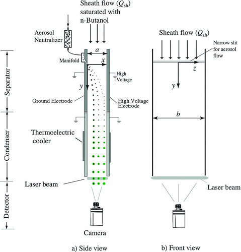
TABLE 1 Dimensions and operating conditions of the FIMS

Dimension or Operating Condition	Value
Distance between separator electrodes, a	11.18 mm
Width of channel, b	127.0 mm
Length of separator, l s	112.1 mm
Length of condenser, l c	319.3 mm
Sheath flow rate, Q sh	13.4 L/min
Aerosol flow rate, Q a	0.268 L/min
Separator electrode voltage, V	700 V
CCD camera frame rate	10.0 Hz

3. CORRECTING THE RECORDED DATA FOR FAST TRANSIENT MEASUREMENTS

Although the FIMS camera can be operated at frame speeds up to 60 Hz, the time resolution of FIMS measurements is limited by non-uniform flow fields and flow mixing that leads to transient errors and the distortion of derived size distribution in transient measurements. An ideal aerosol spectrometer would measure the exact aerosol size distribution at the instant it was sampled. In reality, all in-situ aerosol spectrometers must sample the aerosol through some kind of inlet (which usually includes a sample line), that produces a time delay in the measured data, but more importantly it may also cause mixing of the aerosol sample due to non-uniform flow fields and flow mixing inside the inlet. This mixing will result in particles being detected at different times relative to the time they were sampled, which distorts the measured size distribution of rapid changing aerosols. Furthermore, the particle transit time inside the FIMS separator and condenser is a function of particle size, which causes particles of different sizes to be detected at different times relative to the time they enter the separator.The inlet configuration typically used on the FIMS is shown in Figure 2a.

FIG. 2 Inlet configurations of the FIMS and the CPC.

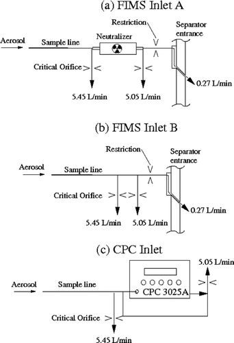
The aerosol is sampled through a sampling tube and a neutralizer before it enters the separator through a narrow slit in the separator wall. The mixing of the aerosol within the inlet, which is defined as the tip of the sampling line to the narrow entrance slit of the FIMS, comes from three major sources. First, mixing of the aerosol within the sampling line occurs due to the non-uniform laminar flow field in the tube, since the flow velocities near the tube wall are much smaller than the flow velocity at the center of the tube. This can be greatly reduced if the flow is turbulent, although this will increase particle losses in the tube. Second, additional particle mixing can occur within the neutralizer due to its shape. The current neutralizer used with the FIMS (Aerosol Neutralizer, Model 3077A; TSI Inc.) is cylindrical and the abrupt expansion at its entrance and contraction at its exit generates secondary flows and further enhances mixing of the aerosol. Third, after the particles pass through the neutralizer, the particles travel through a tube into a small manifold and are distributed into the separator through a narrow slit entrance (approximately 0.25 mm wide and 127 mm long). Therefore, particles that are distributed toward the ends of the slit will enter the separator slightly after particles entering near the center of the slit, causing additional mixing. In transient measurements, the mixing described above causes particles to enter the FIMS entrance slit at different times relative to the time they were sampled at the inlet tip, which leads to smearing of the measurement. The smearing effect causes a time-dependant error in the particle concentration measured in each size bin. If the mixing of the aerosol sample in the inlet is not accounted for, it can not only lead to errors in the number concentration of the size distribution, but also to errors in the characteristic parameters of the distribution such as the geometric mean diameter (GMD), geometric standard deviation (GSD), skewness (SKW), etc. The smearing effect due to the mixing can be corrected by de-convolving the time series of particle counts in each size bin as will be shown in section 3.2.

Another factor leading to error in FIMS transient measurements is the difference in transit times of particles inside the separator and condenser, i.e., from the entrance slit to the detection plane. The velocity profile of the carrier gas (the sheath flow plus aerosol flow) is parabolic in the separator and condenser. Therefore, particles of different electrical mobilities (Z_p ), which travel at different trajectories in the separator and condenser, will have different transit times in the FIMS. If not corrected, this can lead to error in the determined size distribution. Determining the transit time of each particle from theory and correcting the particle detection time can be used to correct this and is shown below. It is important to point out that the impact of the transit time on the measurement is a function of particle mobility, whereas the smearing effect in the inlet is caused by the non-uniform flow field, which, to the first order, affects particles with different mobilities equally.

3.1. Correcting the Transit Time in the Separator and Condenser

An important consideration in the FIMS inversion is the time correction to account for the difference in transit times of the particles with different electrical mobilities. Olfert et al. (2008) showed that the particle transit time in the separator, t _s, is,

while the particle transit time in the condenser before it reaches the detection plane, t _c, is,

where a is the distance between the electrodes, b is the width of the separator and condenser channel, l _c is the distance from the entrance of the condenser to the detection plane, V is the voltage difference across the electrodes, Q _t is the total flow rate (the sheath flow rate (Q _sh) plus aerosol flow rate (Q _a); Q _t=Q _sh+Q _a), Z _p is the particle electrical mobility, and ∗ (Z_p) is the dimensionless distance from the ground electrode (see Figure 1) where the particle has been detected (∗ (Z_p) = x∗ (Z_p) / a) and is a function of the electrical mobility of the particle.

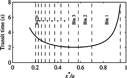
Figure. 3 shows a plot of the total particle transit time in the separator and condenser as a function of the particle detection position for the operating conditions listed in Table 1, with the location of the size bins shown for reference. The figure shows that there is a large difference in transit times between particles that are detected at the center of the channel (Bin 3 and 4, for example) and those near the edge of the channel (Bin 1). To correct this, the time each particle entered the separator is calculated using Equations (1) and (2), and the de-convolution of FIMS mobility measurements is performed on the ‘time-corrected’ data. This is the inversion technique used in Olfert et al. (2008), and will be referred to here as the “standard inversion.” The standard inversion gives the aerosol size distribution at the slit entrance of the separator, and does not take into consideration the smearing effect in the FIMS inlet upstream of the slit entrance.

FIG. 3 Total transit time of a particle in the FIMS as a function of its detection position,

∗ = x∗/a, for the operating conditions shown in Table 1.

3.2. Correcting for Aerosol Mixing in the FIMS Inlet

The above time correction accounts for the difference in particle transit times from the slit entrance to the detection plane. However, as mentioned above, non-uniform flow fields cause mixing of the aerosol in the inlet system, which includes the sampling line, neutralizer, and the entrance manifold. This mixing results in those particles that were sampled at the tip of inlet at one instant to arrive at the slit entrance at different times. The smearing due to these effects can be corrected by de-convolving the time series of particle counts in each size bin (after the transit time inside the FIMS is corrected for as described in Section 3.1). Similar smearing effects are also found in the SMPS system; where, if the voltage scanning time is short, the derived size distributions can be skewed relative to the true distribution due to mixing within the CPC. Russell et al. (1995) corrected for this smearing by deriving an effective system transfer function used in the inversion of the raw particle counts. Collins et al. (2002) approached this same problem by first de-convolving the time series of the raw CPC counts, and then performing the mobility de-convolution (data inversion). A similar technique can be used with the FIMS, where the raw counts in each size bin are de-convolved with respect to time and then the mobility de-convolution is carried out using the inversion routine. Collins et al. (2002) describes in detail the technique for the SMPS system, which was modified for the FIMS and is summarized here.

The particles that enter the FIMS separator slit at one particular time, t, will be dependant on the number of particles that entered the FIMS inlet at all previous times. From the analysis of the digital images and with the application of the time correction mentioned above, the number concentration of the particles classified in size bin i, Cⁱ (t), entering the separator through the slit at time, t, is determined. The unknown concentration, Rⁱ (t'), of particles that enter the FIMS inlet (i.e., the entrance of the sampling line) at a previous time, t', and later classified in size bin i, is related to Cⁱ (t), through the convolution equation;

where Θ(t−t') is the response function defined as the fraction of particles that entered the FIMS inlet at time t' that entered the separator through the narrow slit at time, t. Θ(t−t') can be determined by modeling the expected response of the instrument due to smearing effects, as shown below.

The FIMS captures images at a frame rate, _F (typically 10 Hz), so the particles counted in one frame will be the number of particles counted in a time interval, Δt, equal to 1/ _F. Since the particle count measurements are discrete, Equation (3) can be approximated with the rectangle rule as,

where m and n are indices for times t and t', respectively (i.e., t=mΔt and t'=nΔt).

This can be expressed in matrix form as,

A model is needed to describe the smearing within the FIMS inlet so that the response function can be determined. As shown below with experimental results, the smearing in the FIMS inlet can be modeled as a first-order system. For a first-order system (or instrument), the system output (q _out) at time, t, to an earlier input (q _in) will follow an exponential decay (Doebelin 1966),

where τ is the time constant of the system. Since the FIMS inlet is a first-order system, Equation (6) can be used to derive the Θ function. According to Equation (6), all inputs previous to a particular time will contribute to the output. In reality, only a certain number of time bins, p, previous to the time of interest (mΔt) need to be considered, since the contribution of a much earlier input to the current output is very small. For this work, we have chosen p to be the nearest integer greater than 3τ/Δt. Using Equation (6), the response function will be:

This produces a banded lower-triangular matrix, where the summation of each row equals unity. The second case in Equation (7), is used to conserve the particle concentration at the start of the time series.

Therefore, with C ⁱ and Θ known, Equation (5) can be solved to find the de-convolved particle counts in each size bin, R ⁱ . The equation could be solved directly using forward substitution; however, random errors in the measurement will be greatly amplified making the de-convolved time series data extremely noisy. To reduce the noise, a de-convolution routine with a smoothing criterion can be used (see Kandlikar and Ramachandran (1999) for a review of inversion methods). In this work we have used the Twomey method with the same algorithm used in the inversion of the size distribution, which has previously been described in detail (Olfert et al. 2008). Since the data files can be several hours long with hundreds of thousands of time steps, it is not feasible to solve Equation (5) with the entire data set. Therefore, the data is temporally de-convolved in batches of time on the order of 10τ long, where the first 5τ is not used in order to minimize any effect due to the correction for the start of the time series (see case 2 in Equation [7]). In this work, the inversion routine that includes this temporal de-convolution method (and the correction for the particle residence time above) will be referred to as the `time de-convolved inversion'.

4. EXPERIMENTAL METHOD

The purpose of this work is to understand the dynamic characteristics of the FIMS in order to (1) understand the limitations and errors associated with transient measurements with the FIMS; (2) show that the correction for the particle transit time in the separator and condenser is accurate; and (3) show that smearing effects of the FIMS inlet can be corrected with the time de-convolved inversion. An important parameter needed to accomplish the first and third goals is the time constant of the FIMS inlet, τ. In a first-order instrument, the time constant will determine the transient error of the measured signal due to a transient input, and as shown in Section 3.2, the time constant is needed to de-convolve the time series data to account for the smearing effect. The second goal can be accomplished by measuring the size distribution of an aerosol that is rapidly diluted. When the aerosol is diluted, the number concentration of the aerosol will decrease, but the distribution parameters such as geometric mean diameter (GMD), geometric standard deviation (GSD), skewness (SKW), etc., will remain constant. Since the particle transit time inside the FIMS is a function of particle mobility, rapidly diluting the aerosol will cause a shift in the measured size distribution, if the data were not corrected. Therefore, if the size distribution parameters (GMD, GSD, SKW, etc.) derived using the standard inversion remain constant, then the size bin-dependant time correction for the transit time in the separator and condenser will be accurate.

The time constant of a first-order instrument can be determined by analyzing the response of the instrument to a step change in the input or by examining the instrument's frequency response. Determining the time constant of the FIMS is somewhat complicated by the fact that the FIMS does not measure a single parameter (such as particle number concentration, etc.), but a size spectra, which can be expressed in terms of the total number concentration (N), geometric mean diameter (GMD), geometric standard deviation (GSD), skewness (SKW), etc. As shown earlier, the standard inversion takes into consideration the particle transit time inside the FIMS and gives the size distribution of particles at the slit entrance. The smearing effect of the inlet is caused by non-uniform flow and flow mixing between the tip of the sampling line and the slit entrance, which to the first order, affects particles of different sizes equally. Therefore, the time constant of the FIMS inlet can be determined by measuring an aerosol of any size using the standard inversion.

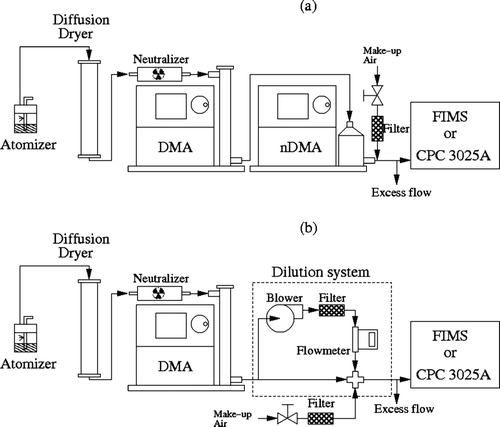
A rapid change in the number concentration of an aerosol can be achieved by either dilution or electrostatic precipitation (with a DMA for example). To produce a step change in the number concentration of an aerosol distribution a serial DMA system can be used where one DMA produces a narrow distribution and the second DMA is instantaneously stepped between the same classification size and a much larger or smaller classification size, where no particles penetrate. In order to measure the frequency response of the FIMS, a sinusoidal oscillation in the number concentration of an aerosol size distribution is used. This can be achieved by using a DMA to produce a constant aerosol size distribution and using a controlled blower and filter to rapidly, and predictably, dilute the aerosol in a sinusoidal manner.

Figure 4a shows the experimental set-up used to produce a step change in the number concentration of an aerosol, which was measured with the FIMS with and without the neutralizer, and with a condensation particle counter (CPC Model 3025A; TSI Inc.). The inlet configuration without the neutralizer is given in Figure 2b. The FIMS measurements were made with and without the neutralizer because the neutralizer is a major contributor to the overall smearing effect of FIMS inlet due to its large internal volume. By making measurements with and without the neutralizer, the relative effect of the neutralizer on the time constant could be determined. In addition, the current TSI neutralizer geometry and configuration are far from optimal for transient measurements. The measurements without the neutralizer show the potential of rapid FIMS measurements when neutralizers with low flow mixing are developed and used. The CPC was included in the measurements because previous studies have measured the time constant of the CPC 3025 (Buzorius 2001; Quant et al. 1992; Wang et al. 2002) and the results will be compared here. In the experiment, sodium chloride (NaCl) particles are generated in an atomizer (Model 3076, TSI Inc.) and dried in a silica gel diffusion dryer. A narrow distribution of particles with a peak at 47 nm was selected with a DMA (Model 3081; TSI Inc.) operating at a sheath flow rate to aerosol flow rate ratio of 10. The aerosol was then passed through a nano-DMA (Model 3085; TSI Inc.) with a sheath flow rate of 20 L/min and an aerosol flow rate of 2 L/min. The voltage on the nano-DMA was controlled with serial commands to step between the classifying voltage for 47 nm particles (∼7000 V) and the maximum voltage of 10000 V, where no particles penetrate. A nano-DMA (with high flow rates) is used as the second DMA to reduce the residence time in the DMA (the transit time in the nano-DMA is 0.12 s). The particles that pass through the nano-DMA are mixed with particle-free dilution air to increase the flow rate in the short sampling line that carries the aerosol to the instruments. The flow rate is increased to reduce the residence time in the sample line and to ensure that the flow in the sample line is turbulent so that smearing in the sampling line is negligible. The flow configurations for the FIMS with the neutralizer (Inlet A), without the neutralizer (Inlet B), and for the CPC are shown in Figure 2.

FIG. 4 Schematic of experimental set-ups used to determine the instrument's step-response (a) and frequency-response (b).

In each set-up, critical orifices control the flow rate in the sampling line. In both FIMS configurations the total flow rate in the sampling line was 10.8 L/min and in the CPC the sampling line flow rate was 10.5 L/min, which resulted in Reynolds numbers of 3180 and 3090, respectively (i.e., turbulent flow). When the FIMS was used with the neutralizer (Inlet A), two critical orifices where used to control the flow (see Figure 2a), so that the flow rate in the neutralizer was 5.32 L/min, which is near the recommended maximum flow rate for the neutralizer (5 L/min).¹ In these experiments, the FIMS can be operated without the neutralizer because the particles will already be charged after they passed through the neutralizer upstream of the DMA; however, the kernel in the FIMS inversion routine must be adjusted to account for the difference in the charge distribution, as explained by Olfert et al. (2008). A restrictor is needed in front of the entrance into the FIMS separator to dampen pressure oscillations in the separator. Since the volume of the separator is large and the aerosol flow rate is small, small pressure fluctuations in the separator can cause large fluctuations in the aerosol flow rate, which can cause large errors in the measured number concentration.

The frequency response of the FIMS was found by measuring a size distribution that was diluted in such a way that the number concentration of the aerosol varied sinusoidally (see Figure 4b). The frequency response can be used not only to determine the time constant of the instrument but also to verify that the time correction for the particle transit time from slit entrance to the detection plane is accurate. When the aerosol is diluted, the distribution parameters GMD, GSD, and SKW will remain constant. As the smearing effect is caused by non-uniform flow inside the inlet, it is independent of particle size. As a result, the shape of the particle size distribution at the separator slit will also remain constant. If the correction of the particle transit time from the entrance slit to the detector is accurate, the distribution parameters derived using the standard inversion will remain constant despite the smearing effect of inlet. Therefore, the measured GMD, GSD, and SKW signals can be analyzed to verify the accuracy of the correction. In the experimental set-up, the aerosol was generated and dried using the same method as above. A wide aerosol size distribution was selected by passing the aerosol through a DMA (Model 3081; TSI Inc.) with a sheath flow rate of 2 L/min and an aerosol flow rate of 2 L/min. The peak of the distribution was set to 48 nm with the DMA. The aerosol was diluted with the system shown in the figure, where the blower was used to dilute the aerosol in a sinusoidal manner. The blower was controlled in a feedback PID control system implemented in LabVIEW, using a calibrated flowmeter (V-10LPM-O; Alicat Scientific). In such a dilution system, it can be shown that the required dilution flow rate through the blower (Q_d ) to produce a sinusoidal change in the number concentration is,

where f_d is the frequency of the sinusoidal dilution, and Q _d,max and Q _d,min are the maximum and minimum dilution flow rates, respectively. The maximum and minimum dilution flow rates used in this work were 1.9 L/min and 1.5 L/min, respectively. The maximum frequency that could be controlled in this manner was 0.33 Hz. As before, additional dilution flow was added to the aerosol to ensure that the flow in the tube to the instruments was turbulent.

In both set-ups, the FIMS was operated with the operating conditions shown in Table 1. Images were recorded with a frequency of 10 frames per second (10 Hz). To improve counting statistics, two frames worth of data were combined for the inversion of each size distribution (see Olfert et al. 2008). Therefore, the FIMS data is shown in time steps of 0.2 s. The number concentration measured by the CPC 3025A was determined by recording the pulses (from the “PULSE OUTPUT” BNC connection on the back of the CPC) in a LabVIEW data acquisition system and averaging over a time step of 0.2 s.

5. EXPERIMENTAL RESULTS AND DISCUSSION

5.1. Verifying the Correction for the Particle Transit Time in the Separator and Condenser

One goal of this work is to verify that the time correction for the particle transit time from the separator entrance to the detection plane is accurate. This can be done by examining the size distribution parameters derived from the standard inversion as an aerosol is rapidly diluted. When an aerosol is diluted sinusoidally the number concentration rapidly increases and decreases but the size distribution parameters of the aerosol (e.g., GMD, GSD, and SKW) will remain constant. The smearing of the aerosol in the FIMS inlet is independent of the particle size; however, the transit time in the separator and condenser is a function of the particle electrical mobility. Therefore, if the transit time is not corrected, the measured distribution parameters will change with the dilution. If, however, a correction of the particle transit time from the slit to the detector is used, as it is in the standard inversion, and it is accurate, then the measured size distribution parameters will remain constant with time.

Figure 5a–b shows the total aerosol number concentration as a function of time and the size distribution at t= 5 s measured by the FIMS; respectively, for the aerosol diluted at f _d= 0.33 Hz (the highest frequency used in this work).

FIG. 5 (a) Number concentration measured by the FIMS for sinusoidal dilution of a size distribution with a frequency of 0.33 Hz; and (b) the size distribution of the aerosol at t = 5 s. (c)–(e) The frequency spectrum of the GMD, GSD, and SKW about their mean (i.e.,

; where |Y _GMD(f)| is the single-sided amplitude spectrum of y _GMD(t) determined by fast Fourier transform (FFT)) of the measured distribution with the standard inversion (labeled ‘Standard’) and without the time correction used in Equations (1) and (2) (labeled ‘Uncorrected’).

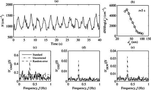
Figure 5c–e shows the frequency spectrum of the GMD, GSD, and SKW of the measured size distribution over the same time period, when the standard inversion is used and when the time correction discussed in Sec. 3.1 is not used (labeled “uncorrected”). The frequency spectrum is determined by taking the Fourier transform or FFT of each time series for each parameter about its mean. For reference, a representative random error is also shown on the frequency spectrum, which was defined as the mean spectrum amplitude plus one standard deviation. If the measured parameters were changing with respect to the dilution frequency, one would notice a spike in the frequency spectrum at the dilution frequency, f _d (in this case f _d= 0.33 Hz). First, considering the standard inversion, there seems to be little correlation with the dilution frequency and changes in the GMD, while there is a small correlation with GSD and SKW with the dilution frequency. For comparison, the frequency spectrum of the data without the time correction is shown. It is apparent in this case that the GMD, GSD, and SKW oscillate at the dilution frequency. This is expected since the particle transit time inside FIMS is size-dependant (see Figure 3), which leads to changes in the shape of the size distribution. The error in the distribution parameters can be quantified by dividing the amplitude of the parameter at the dilution frequency (e.g., |Y _GMD(f _d)|) by the mean parameter value (e.g., GMD).

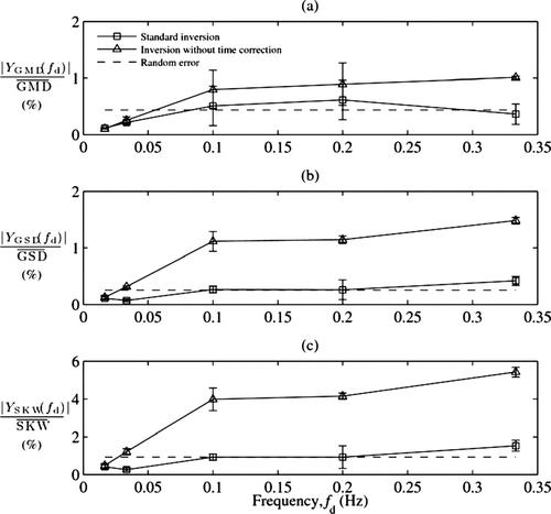
Figure 6 shows the percent error in each of the variables over the range of dilution frequencies. The representative random error is also plotted for comparison (the uncertainties and error bars reported through out this work are one standard deviation of the data from three repeated tests). The figure shows that for the standard inversion, the error in the parameters is only slightly above the random error in only the case with the fastest dilution. This shows that Equations (1) and (2) (used in the standard inversion) describe the particle transit time quite accurately.

FIG. 6 Measured error in the distribution parameters GMD, GSD, and SKW as a function of the dilution frequency.

5.2. Time constant of the FIMS

The time constant of the FIMS inlet is needed to understand the errors associated with transient measurements and to temporally de-convolve the data. Since the transit time correction is used to calculate the time the particles enter the separator, the only source of time delays and smearing will be in the FIMS inlet. Therefore, if we experimentally determine the total time constant of the FIMS using the standard inversion (the inversion using the transit time correction), then that total time constant will simply be the time constant of the FIMS inlet. One method used to determine the time response of an instrument is to observe the response of the instrument to a step change in the instrument input. Quant et al. (1992), Buzorius (2001), and Wang et al. (2002) used this technique to find the time response of various condensation particle counters.

Figure 7 shows the response of the CPC 3025A and the FIMS with and without the neutralizer, to a step change in the number concentration. The experimental data were fit with an exponential decay, which is the expected response of a first-order instrument to a step-change:

where N _out is the aerosol concentration measured by the instruments, N ₀ is the aerosol concentration before t ₀, where t ₀ is the time the step in concentration is first detected. For FIMS measurements, N is calculated by integrating the size distribution derived using the standard inversion. The data was fit using Equation (9) with a chi-squared minimization technique, where t ₀ and τ were adjustable parameters. The time constants determined in this way were: 0.14 ± 0.02 s for the CPC 3025A, 0.76 ± 0.10 s for the FIMS without the neutralizer, and 1.69 ± 0.10 s for the FIMS with the neutralizer. Buzorius (2001) also determined the time constant of the CPC 3025A to be 0.14 s using the same technique, while Quant et al. (1992) measured the time constant of a CPC 3025 to be 0.27 s using a slightly different technique.² Wang et al. (2002) used a spark-source aerosol generator and measured the time constant of 0.174 ± 0.005 s for a CPC 3025. For comparison, the time constant of the CPC 3010 (TSI Inc.) as determined by Buzorius (2001), is also shown on the figure and is similar to the time constant of the FIMS without the neutralizer.

FIG. 7 Response of the FIMS and CPC to a step-change in aerosol number concentration. The solid lines represent the fit of the data to Equation (9).

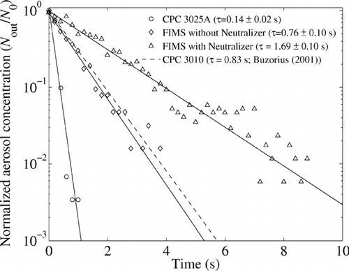
It is immediately obvious from the figure that the time response of the FIMS is much slower when the neutralizer is used. As mentioned above, this is due to the mixing of the aerosol in the neutralizer due to its shape. The current neutralizer used in the FIMS is designed to be used with a DMA or SMPS system, where the smearing due to the neutralizer is not usually important given the slow response of SMPS systems. In practice, a FIMS neutralizer could be designed where mixing was minimized.

Another important aspect of Figure 7 is that the theoretical response of a first-order system (Equation [9]) fits the FIMS data well (the increasing scatter from the fit at lower particle concentrations is due to decreasing counting statistics). This shows that the response of the FIMS is close to that of a first-order instrument. Therefore, the response function shown in Equation (7) will provide a good representation of the response of the instrument for the temporal de-convolution.

Another technique to determine the time response of an instrument is to measure the attenuation of a sinusoidal input as the function of the frequency of the input. It can be shown (see Doebelin (1966) for example) that the frequency-response of an ideal first-order instrument will be,

where K is the steady-state gain of the instrument (K=1 for the FIMS and CPC), and N _out and N _in are the output and input aerosol concentration of the instrument, respectively. Equation (10) shows that for larger time constants the amplitude ratio (or the magnitude of Equation (10) decreases; this is known as attenuation. Furthermore, as the time constant increases the phase angle (or the delay between the input and output signal) increases.

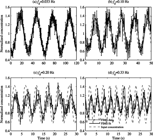
Figure 8 shows the response of the FIMS to a sinusoidal input that was created by diluting an aerosol that was pre-classified with the DMA. The number concentration from the FIMS standard inversion is normalized (N _out / N _out) and fit with a sine wave using a chi-squared minimization technique; both the raw measurements and the fit are shown in the figure. For comparison, the input aerosol concentration is shown, where the amplitude of the input was determined experimentally by measuring the aerosol concentration at Q _d,max and Q _d,min; and the phase angle between the measured response and the input was determined from Equation (10). The figure shows that as the dilution frequency (f _d) increases, the amplitude of the measured concentration decreases and the phase angle increases.

FIG. 8 Normalized number concentration (N _out / N _out) measurements of the FIMS (without the neutralizer) at four dilution frequencies.

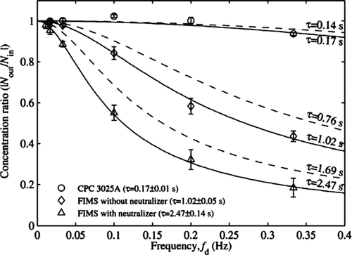
Figure 9 shows the frequency-response curve of the CPC 3025A and the FIMS with and without the neutralizer. The frequency-response curve shows that the concentration ratio (or the magnitude of Equation (10); |N _out/N _in|) decreases as the frequency of the dilution increases. For instruments with high time constants the attenuation can be quite substantial. For example, at a frequency of 0.33 Hz, the FIMS signal was attenuated 56% when the neutralizer was not used and 82% when the neutralizer was used. The lines in the figure represent the theoretical frequency-response from Equation (10) with various time constants. The solid lines represent the fit of the experimental data with the theory and the dashed lines correspond to the time constants that were determined using the step-response experiment described above. The time constants determined from the fit of the frequency-response data were: 0.17 ± 0.01 s for the CPC 3025A, 1.02 ± 0.05 s for the FIMS without the neutralizer, and 2.47 ± 0.14 s for the FIMS with the neutralizer. It is apparent that the experimental data fits the theoretical response well; however, the time constants determined from this frequency-response data are larger than those determined from the step-response data. This could be caused by two factors; (1) the dilution system may cause some additional smearing which is not observed in the step-response set-up, and (2) the instruments are not perfectly first-order. Buzorius (2001) measured the frequency-response of a CPC 3025A and a modified CPC 3010 using a different method.³ He also found that the time constant determined with the frequency-response experiments were larger for the CPC 3010 than the time constant determined with the step-response experiment. Although the time constants determined from this frequency-response data are greater than those determined from the step-response data it is interesting to note that time constant measured by Wang et al. (2002) for the CPC 3025 (0.174 ± 0.005 s) agrees well with the frequency-response time constant measured in this work with the CPC 3025A (0.17 ± 0.01 s).

FIG. 9 Frequency-response curves of the CPC 3025A and FIMS with and without the neutralizer. (Solid lines represent the fit of the data. Dashed lines represent the frequency-response of instruments with the time constants found with the step-change experiment.)

5.3. Temporal De-Convolution of FIMS Data

For measurements of rapidly changing aerosols, the smearing effect of the FIMS inlet can cause errors in the measured size distribution using the standard inversion because the aerosol sampled at one instant will enter the slit entrance over a period of time. The magnitude of this transient error will depend on the rate of change of the particle concentration. This will cause errors, not only in the distribution's number concentration, but also in its determined shape. By de-convolving the time series of number concentration measured in each size bin, the transient error is greatly reduced (ideally to zero) and the determined size distribution will be much closer to the actual distribution. Section 3.2 described the method that can be used to temporally de-convolve the number concentration in each size bin. This method was used on the FIMS data recorded in the frequency-response measurements described above.

Figure 10 shows an example of the temporally de-convolved FIMS data with a dilution frequency of 0.2 Hz. The figure shows the data both before and after temporal de-convolution is applied using the method described above with a time constant of τ _d= 1.0 s (where τ _D represents the time constant used in the de-convolution algorithm). The time constant of the FIMS is approximately 1.0 s (as determined from the frequency-response experiment), so using a de-convolution time constant of τ _d=1.0 s should reconstruct the actual aerosol input. Figure 10bshows that the amplitude and phase of the result from time de-convolved inversion is very close to the actual input.

FIG. 10 Example of the temporally de-convolved FIMS measurements (without the neutralizer) for an aerosol distribution diluted at a frequency of 0.2 Hz.

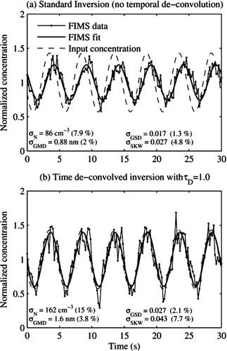
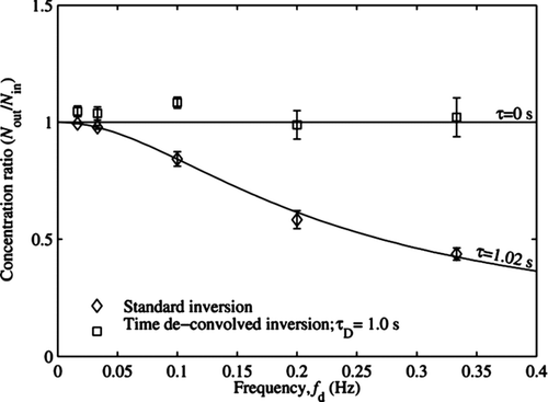
Figure 11 shows the frequency-response curves for the FIMS (without the neutralizer) both with the standard inversion and with the time de-convolved inversion over a range of dilution frequencies. The figure shows that the frequency-response of the FIMS is close to 1 when the time de-convolved inversion is used. As mentioned in Sec. 3.2, one potential problem with temporal de-convolution of the data is that random noise in the measurement is amplified. Inset in each sub-figure in Figure 10 are the standard deviation of the size distribution parameters, σ, (N, GMD, GSD, and SKW) of the examples. (In the case of N, it is the standard deviation from the fit of the data; the other parameters will remain constant with time.) Comparing the standard inversion to the time de-convolved inversion, one can see that the standard deviations in the distribution parameters nearly double. It should be noted that the error in the measured size distribution will depend on the size distribution and the rate of change of the aerosol. For example, if the aerosol concentration was rapidly increasing, the contribution of previous time bins to the current time bin would be small and the noise in the time de-convolved inversion would be small. If, however, the aerosol concentration was rapidly decreasing the contribution of previous time bins to the current time bin would be relatively large and the noise in the time de-convolved inversion would be larger. Therefore, temporal de- convolution of data should be used with caution and only when the benefit of the reduction in the transient error outweighs the increase in the random noise.

FIG. 11 Frequency-responses of the FIMS (without the neutralizer) both before and after temporal de-convolution is applied with a time constant of 1.0 s. (Solid lines represent the theoretical frequency-response of an instrument with a time constant of τ-0 s and τ-1.02 s, respectively.)

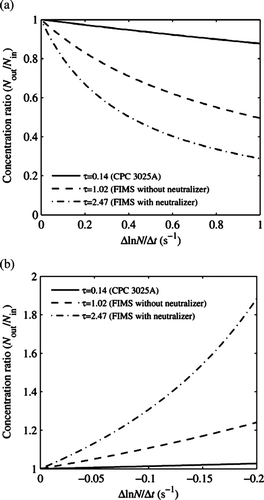
In addition to the aerosol with sinusoidal variation in its concentration, the response of the FIMS to another type of transient aerosol, of which the fractional change rate of the particle concentration is constant, was studied. The transient error of the FIMS measurement using the standard inversion can be expressed as a function of the fractional change rate of the concentration, in other words, the response of the instrument to an exponential change in the aerosol number concentration (ΔlnN/Δt). The transient error of a general first-order instrument to an exponential ramp in the input signal is presented in Appendix A. The analysis shows that after an initial transient period, the relative transient error of the instrument (N _out/N _in) to an exponentially changing concentration reaches a steady-state value (see Figure A1).

Figure 12 hows the theoretical relative transient error of the CPC and FIMS to a steady exponential increase and decrease in the number concentration (ΔlnN/Δt). As was seen in the frequency-response curve, smaller values of τ will result in less transient error. This information can be used as a guideline for determining if the time de-convolved inversion is needed. This can be done by analyzing the number concentration measured by the instrument to see if the fractional rate change in the number concentration will cause a significant transient error. For example, for an exponential increase of ΔlnN/Δt= 0.11 s⁻¹ with a FIMS with a time constant of τ= 1.02, the transient error will be 10% (see Figure 12a). Therefore, if faster change rates are measured then the transient error will be higher and the time de-convolved inversion should be used. If the time de-convolved inversion is used, the solution should be compared to the standard inversion to determine if the benefit of the reduction in the transient error outweighs the increase in the random noise. As an example we can consider the frequency-response data shown in Figure 10. An analysis of the experimental data shown in Figure 10a reveals that the maximum fractional rate of change in the measured signal is 0.61 s⁻¹. In reality the actual fractional rate of change maybe higher than the measured rate change if the concentration change is brief and the instrument did not have time to reach the steady-state value of the relative transient error. In this particular example, the actual input is known and the maximum fractional rate of change is 0.62 s⁻¹, which is slightly above the measured value. In any case, the measured fractional rate of change indicates that there will be significant transient error (approximately 40%; see Figure 12a) and therefore the data should be temporally de-convolved. By comparing the standard inversion to the time de-convolved inversion in Figure 10, it is apparent that the time de-convolved inversion captures the change in the particle concentration with a relatively modest increase in the random noise, and therefore using the time de-convolved inversion was justified.

FIG. 12 Theoretical response of a first-order instrument to an (a) exponential increase and (b) exponential decrease in input with various time constants.

6. SUMMARY

It is necessary to know the dynamic characteristics of an instrument so that the errors associated with transient measurements are known and so that the data can be corrected. The time response of the FIMS is limited by the smearing of the aerosol in the inlet and also due to the difference in transit times of particles from the FIMS slit entrance to the detection plane. It was shown experimentally that the difference in transit times could be accurately corrected by using a simple model of the particle trajectories. For transient measurements, the time constant of the FIMS inlet is needed to understand the errors associated with the smearing effect and to temporally de-convolve the data. The time constant of the FIMS inlet and a CPC 3025A was determined by measuring both the step-response and frequency-response of the instruments. The time constants determined from the step-response were: 0.14 ± 0.02 s for the CPC 3025A, 0.76 ± 0.10 s for the FIMS without the neutralizer, and 1.69 ± 0.10 s for the FIMS with the neutralizer. The time constants determined from the instrument frequency-response were: 0.17 ± 0.01 s for the CPC 3025A, 1.02 ± 0.05 s for the FIMS without the neutralizer, and 2.47 ± 0.14 s for the FIMS with the neutralizer. Discrepancies between these two measurements maybe due to a small amount of additional smearing in the dilution system used in the frequency-response experiment, or perhaps the FIMS inlet is not an ideal first order system. The frequency-response curve of the FIMS shows that the attenuation of the number concentration is significant at high frequencies. For example, at a frequency of 0.33 Hz, the FIMS signal was attenuated 56% when the neutralizer was not used and 82% when the neutralizer was used. It was shown that the attenuation (or the transient error) could be eliminated by de-convolving the time series of particle measurements. However, random noise is amplified in the measurement when the time de-convolved inversion is used. Therefore, temporal de-convolution of data should be done with caution and only when the benefit of the reduction in the transient error outweighs the increase in the random noise. As a guideline to determine if the temporal de-convolution of the FIMS data is needed, the fractional rate of change in the measured number concentration can be analyzed to see if the rate exceeds some limit corresponding to an unacceptable level of transient error. If this limit is exceeded, the data should be analyzed with the time de-convolved inversion and the transient and the random errors can be compared to see if a more accurate size distribution is constructed.

APPENDIX A. THE RESPONSE OF A FIRST-ORDER INSTRUMENT TO AN EXPONENTIALLY CHANGING INPUT

The response of first-order instruments to step, ramp, impulse, and sinusoidal inputs are given in Doebelin (1966). However, for aerosol instrumentation, one would like to know the response of an instrument to aerosol concentrations that are changing exponentially, since an exponential change in number concentration represents a constant increase in the fractional change of the concentration with respect to time. This appendix derives the response of a first-order instrument to an input that is changing exponentially. A first-order instrument is defined as an instrument that follows the equation,

where, q _in is the instrument input, q _out is the instrument output, τ is the time constant of the instrument, and K is the static sensitivity, that is the amount of output per unit input when the input is steady. The response of the instrument, q _out, can be determined by solving the differential equation for various inputs.

An exponential change in the input can be expressed as,

where q ₀ is the initial input, t is the time, t ₀ is the time the exponential change began, and c ₁ is an arbitrary constant. If we consider that the input has changed to a new value, q _f, at some time t=t ₀+Δt, then the equation becomes,

Equation (A1) can be solved using the method of undetermined coefficients where the solution is found by the superposition of the general solution of the homogeneous equation and the particular equation. The general solution of the corresponding homogenous equation is,

where c ₂ is an arbitrary constant.

To find the particular solution, we can guess a solution of the form,

where c ₃ is a constant. The constant c ₃ is determined by substituting Equations (A3) and (A5) into Equation (A1). This results in the particular solution,

Therefore the general solution to Equation (A1) will be,

The constant c ₂ is found using the initial condition that at t=t ₀, q _out=q ₀, resulting in,

The ratio between the instrument output and the instrument input (or the relative transient error, or the relative error due to the transient input) is,

Figure A1 shows the response of a first-order instrument to an input that is exponentially increasing or decreasing. In this example (and for the FIMS and CPC) the static sensitivity is unity (K= 1). The figures show that after an initial transient period, the instrument output will rise or fall at the same rate as the instrument input. Therefore, after some time, the relative error due to a transient input will approach a constant or steady-state value (i.e., the relative error will remain constant with respect to time even though the input signal is transient). For an exponentially increasing signal (Δlnq/Δt> 0), the contribution of the first term in Equation (A9) decreases in time and the relative transient error (q _out/q _in) approaches . The steady-state relative transient error for an exponentially increasing signal is plotted in Figure 12a as a function of the rate of change (Δlnq/Δt) for the time constants of the CPC 3025A and the FIMS. For an exponentially decreasing signal (Δlnq/Δt< 0), finding the steady-state relative transient error is complicated by the fact that the contribution of the first term in Equation (A9), may increase with respect to time, depending on the values of τ and Δlnq/Δt. Therefore, a pseudo steady-state relative transient error was determined by calculating the relative transient error when the logarithm of the slope of the output signal (q _out) reached 95% of the logarithm of the slope of the input signal (q _in), i.e., when . Figure 12b shows the pseudo steady-state relative transient error for an exponentially decreasing signal as a function of the rate of change for the time constants of the CPC 3025A and the FIMS.

FIG. A1 Response of a first-order instrument to an (a) exponentially increasing and (b) exponentially decreasing ramp function. (Note: The y-axis is on a logarithmic scale.)

This work was supported by the Office of Biological and Environmental Research, Department of Energy (DOE), under Contract DE-AC02-98CH10866, and the Laboratory Directed Research and Development program at the Brookhaven National Laboratory (BNL). BNL is operated for the DOE by Battelle Memorial Institute. Jason Olfert also acknowledges partial support from the Goldhaber Distinguished Fellowship from Brookhaven Science Associates. The authors also wish to acknowledge Dr. Peter Takacs for his help with the optics on the FIMS.

Notes

1. Ideally, the flow rate in the neutralizer would be 5 L/min to ensure that the aerosol had sufficient residence time to become fully neutralized, yet short enough to minimize mixing. However, due to the limited selection of orifices on hand, the nearest flow rate that could be achieved in the neutralizer was 5.32 L/min. This higher than recommended flow rate may result in the aerosol not achieving complete charge equilibrium, which might result in a small shift in the measured distribution. However, this is not important in this work since the absolute value of the measured distribution is not important, but rather the measured change in the distribution.

2. Quant et al. (1992) report a “time to 5%” of 0.8 s for step-change down in the input concentration. This equates to a time constant of 0.27 s for a first-order instrument. The step-change was produced by sampling ambient and particle-free filtered air through an electrically-operated three-way valve.

3. Buzorius (2001) measured the frequency response of the CPCs by using two DMAs. The first DMA was fixed to provide a steady-state triangular aerosol distribution, which was then classified by a second DMA, with a narrower transfer function, whose voltage was sinusoidally oscillated between the peak concentration and a lower concentration.

REFERENCES

- Buzorius , G. , Rannik , Ü. , Mäkelä , J. M. , Keronen , P. , Vesala , T. and Kulmala , M. 2000 . Vertical Aerosol Fluxes Measured by the Eddy Covariance Method and Deposition of Nucleation Mode Particles Above a Scots Pine Forest in Southern Finland . J. Geophys. Res. , 105 : 19,905 – 19,916 .
- Buzorius , G. 2001 . Cut-off Sizes and Time Constants of the CPC TSI 3010 Operating at 1–3 lpm Flow Rates . Aerosol Sci. Technol. , 35 : 577 – 585 .
- Collins , D. R. , Flagan , R. C. and Seinfeld , J. H. 2002 . Improved Inversion of Scanning DMA Data . Aerosol Sci. Technol. , 36 : 1 – 9 .
- Doebelin , E. O. 1966 . Measurement systems: Application and design , New York : McGraw-Hill .
- Horst , T. W. 1997 . A simple Formula for Attenuation of Eddy Fluxes Measured with First-Order-Response Scalar Sensors . Boundary Layer Meteorol. , 82 : 219 – 233 .
- Kandlikar , M. and Ramachandran , G. 1999 . Inverse Methods for Analysing Aerosol Spectrometer Measurements: A Critical Review . J. Aerosol Sci. , 30 : 413 – 437 .
- Kulkarni , P. and Wang , J. 2006a . New Fast Integrated Mobility Spectrometer for Real-Time Measurement of Aerosol Size Distribution – I: Concept and Theory . J. Aerosol Sci. , 37 : 1303 – 1325 .
- Kulkarni , P. and Wang , J. 2006b . New Fast Integrated Mobility Spectrometer for Real-Time Measurement of Aerosol Size Distribution: II. Design, Calibration, and Performance Characterization . J. Aerosol Sci. , 37 : 1326 – 1339 .
- Olfert , J. S. , Kulkarni , P. and Wang , J. 2008 . Measuring Aerosol Size Distributions with the Fast Integrated Mobility Spectrometer . J. Aerosol Sci. , Accepted by the, doi: 10.1016/j.jaerosci.2008.06.005
- Quant , F. R. , Caldow , R. , Sem , G. J. and Addison , T. J. 1992 . Performance of Condensation Particle Counters with Three Continuous-Flow Designs . J. Aerosol Sci. , 23 : S405 – S408 .
- Russell , L. M. , Flagan , R. C. and Seinfeld , J. H. 1995 . Asymmetric Instrument Response Resulting From Mixing Effects in Accelerated DMA-CPC Measurements . Aerosol Sci. Technol. , 23 : 491 – 509 .
- Wang , J. , McNeill , V. F. , Collins , D. R. and Flagan , R. C. 2002 . Fast Mixing Condensation Nucleus Counter: Application to Rapid Scanning Differential Mobility Analyzer Measurements . Aerosol Sci. Technol. , 36 : 678 – 689 .