Numerical Simulation of Particle Dispersion in the Wake of a Circular Cylinder

Abstract

In this article, numerical simulation of the Navier-Stokes equations was performed for the large-scale structures of a two-dimensional temporally developing cylinder flow and the associated dispersion patterns of particles were simulated. The time-dependent Navier-Stokes equations were integrated in time using a mixed explicit-implicit operator splitting rules. The spatial discretization was processed using spectral-element method. Non-reflecting conditions were employed at the outflow boundary. Particles with different Stokes numbers were traced by the Lagrangian approach based on one-way coupling between the continuous and the dispersed phases.

The simulation results of the flow field agree well with experimental data. Due to the effects of the coherent structures, the particles demonstrate a more organized dispersion process in the space and a periodic dispersion characteristic in the time. Particle dispersion increases with the flow Reynolds number and so does for particle concentration, which is independent of particle size. However, for particles at different Stokes numbers, the dispersion patterns are different. The particles at smaller Stokes number congregate mainly in the vortex core regions and the particles at larger Stokes number disperse much less along the lateral direction with the even distribution. The higher density distribution at the outer boundary of large-scale vortex structure characterizes the dispersion pattern of particles at the Stokes numbers of order of unity. Furthermore, these particles disperse largely along the lateral direction and show the nonuniform distribution of concentration.

INTRODUCTION

The transport of particles in laminar and turbulent flows such as bluff body wakes is a universal phenomenon found in many natural and technological flow systems, with many industrial applications such as drying and combustion processes where particle-dispersion characteristics are critical. In coal combustion systems and coal liquefaction-gasification pipelines, the erosion of material by solid particle impact is an important problem. Growing environmental concern and stricter regulatory legislation has promoted renewed interest in controlling dispersion of contaminants in the wakes of free-standing structures. Hence understanding the large-scale vortex dynamics and predicting the particle dispersion in bluff body wake flows are of interest both fundamentally and for simulation purpose.

The problem of particulate flow over a bluff body can be mainly divided into two parts. The first part consists of the nature of the solid surface impact and the material erosion. Considerable research has been done on the prediction of erosion of bluff body due to particle impacts (Ilias and Douglas 1989; Schuh et al. 1989; Yao et al. 2000; Fan et al. 2002). The second part consists of the particle trajectories. Brandon and Aggarwal (2001) numerically simulated particle transport and deposition in an unsteady particle laden flow over a square cylinder placed in a channel using a staggered-grid control volume approach. They analyzed the impact of Stokes number and Reyonlds number on particle dispersion. However, they did not provide the relationship between particle motion and flow field so the mechanism of particle dispersion in the wake has not been fully discovered. Richmond-Bryant et al. (2006) estimated concentration of particles with low St in the wake of circular cylinder using the steady state Reynolds Averaged Navier-Stokes (RANS) renormalized k ∼ ε model. They found the mechanism of particle interaction with the boundary layer. Particles transported into the boundary layer under the effect of turbulent diffusion, turbophoresis, and/or inertial forces and then separated from the cylinder with the airflow and travelled in a sheath around the periphery of the near wake to converge at the downstream edge of the near wake. However, due to shortcomings of the k ∼ ε model, inaccurate modeling of the turbulence kinetic energy profile in the boundary layer produced overestimation of turbulent particle diffusion around the cylinder wall and the simulation results had large discrepancies with experimental data. Salmanzadeh et al. (2007) investigated particle trajectories and deposition rates on the obstruction and duct walls in a laminar unsteady channel flow with a rectangular obstruction using a finite volume method.

The prediction of particle dispersion and the associated effects of the large-scale structures have been extensively studied by numerical (Uthuppan et al. 1994; Aggarwal 1994; Chang and Kailasanath 1996) and experimental techniques (Longmire and Eaton 1992; Lazaro and Lasheras 1992). Crowe et al. (1985) introduced the Stokes number of particles to show that particles with small Stokes number closely follow the flow and that, conversely, particles with intermediate Stokes number would be dispersed significantly faster than the fluid motion due to the centrifugal effects created by the organized vortex structures. The different dispersion patterns for particles with different orders of Stokes numbers were also found in the two-dimensional experimental and numerical studies by Chein and Chung (1988) and Wen et al. (1992). Squires and Eaton (1991) simulated a homogeneous isotropic nondecaying turbulent flow-field by imposing an excitation at low wave numbers, and studied the effects of inertia on particle dispersion. They used the DNS procedure to study the preferential microconcentration structure of particles as a function of Stokes number in turbulent near wall flows. Elghohashi (1994) simulated particle dispersion in decaying isotropic and homogeneous turbulence using a spectral method and finite-difference schemes. Recently, Ling et al. (1998) and Fan et al. (2001) traced particles with different Stokes numbers in a temporal mixing layer using direct numerical simulation method and both demonstrated that particle dispersion patterns are strongly governed by large-scale vortex structures and three-dimensionality.

The preferential concentration of particles in turbulent eddies have been widely studied. Eaton and Fessler (1994) reviewed studies of dilute, particle-laden flows which include measurement of the instantaneous concentration field. Many researchers (Wen et al. 1992; Longmire and Eaton 1992; Ling et al. 1998; Fan et al. 2002) examined simple free shear flows which are dominated by large-scale, two-dimensional, or axisymmetric vortices. All of these researchers have observed highly organized particle concentration fields for Stokes numbers on the order of one. Particles are flung away from the vortex cores and in many cases collected in rings surrounding the vortices. In the jet and wake flows the particles are concentrated in the highly strained saddle region between successive vortices.

So far, particulate flow around a bluff body has less been reported. In the present study, a particle-laden flow around a circular cylinder was simulated using a numerical simulation solution of the Navier-Stokes equations coupled with Langrangian particle tracking. The major objective is to study the fluid-particle characteristics and examine the availability of two-dimensional numerical simulation method in two-phase coherent vortex structures. Particle dispersion modes at different Stoke numbers in the wake of circular cylinder were investigated. Some quantitative statistics of flow and particle fields were made to reveal the two-phase flow characteristics. The vortex dynamics in the near wake and the different particle dispersion patterns were focused on.

FORMULATION AND NUMERICAL SCHEME

Flow-Field Simulation

Fluid Equations

For an incompressible viscous fluid flow past a circular cylinder, Navier-Stokes equations are considered as the governing equations. Variables considered in the physical motion are normalized as follows:

where R is the radius of the cylinder, U _o is the uniform stream velocity and ρ₀ is the fluid density. Then the continuity equation and the time-dependent Navier-Stokes equations are written in conservative form as:

where V is the velocity (u, v) and Re, the Reynolds number is defined as where υ is the kinematic viscosity.

Boundary Conditions

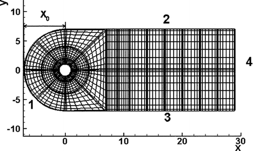
The outlines of the physical domain boundary are specified in Figure 1 in particular that they are fictitious and far from the cylinder. The line numbered 1 is the inflow boundary with an initial condition as u = 1, v = 0. Lines 2 and 3 refers to the top and bottom boundary at y-direction, respectively. Along the two lines, a Neumann-type boundary condition was adopted for the u-component and a Dirichlet-type boundary condition was taken for v-component: ∂ u/∂ y = 0, v = 0. The boundary condition v = 0 effect on the simulation has been justified in the latter section. Line 4 is the outflow boundary and non-reflecting conditions were employed here. In detail, a buffer was set up closed to the outflow boundary and flow viscidity herein was divided into two parts: x-component and y-component. The value of viscidity at x-component decreases progressively and reaches zero at the outflow boundary. This process can ensure the governing equation being parabolic and prevent the upper flow from the diffusing effect by perturbing wave behind. On the contrary, the viscidity of y-component increases gradually at the streamwise direction and introduces diffusing effect on the flow. In principle, the buffer is assumed so long that the following conditions meet at the outflow boundary: ∂ u/∂ x = 0,∂ v/∂ x = 0, p = 0. In addition, the buffer is connecting with the physical domain smoothly to avoid the reflecting effect.

FIG. 1 A sketch of the computational domain.

Numerical Procedure

Time-Discretization

The time-discretization of the governing equations was to employ the mixed explicit/implicit time-integration rules, which can be implemented in three steps:

where are intermediate velocity fields defined in Equations (5) and (6), J _e , J _i are the parameters characterized the accuracy of the overall scheme denoting the individual accuracy of the explicit integration (nonlinear terms) and the implicit integration (viscous terms), respectively, α _q , β _q are implicit/explicit weight-coefficients for the stiffly stable scheme and γ₀ is a weight coefficient of the backwards differentiation scheme. In present research, the process of time-discretization was implemented by third order with the parameters listed below.

Table

γ 0	α 0	α 1	α 2	β 0	β 1	β 2
11/6	3	−3/2	1/3	3	−3	1

Taken the divergence of Equation (6) and combined with the continuity Equation (2), a Poisson equation for the pressure can be obtained:

along with the consistent high-order pressure boundary condition:

which ensures that the divergence is equated to zero on the solid surface. As a result, equations were translated to the Hemholtz form Equations (7) and (8) in the term of V and P. In this work, the time step was set a constant value 0.01.

Spatial Discretization

The spatial discretization of Equations (7) and (8) as Hemholtz form was processed by the method of static condensation for the system matrix. In summary, the standard spectral element discretization the computational domain was broken up into a series of quadrangular elements in two dimensions, which were mapped isoparametrically to canonical squares. Field unknowns and data with the geometry, velocity, and pressure were then expressed as tensorial products in terms of high-order Lagrangian interpolants through Chebyshev collocation points. The final system of discrete equations was then obtained via a Galerkin variational statement by Korczak and Patera (1986).

Further details of the mathematical model employed, and the numerical algorithm and its implementation, may be found in the work (Yao 2002; Yao et al. 2003).

Particle Phase Simulation

Prediction of the solid phase uses a Lagrangian particle tracking approach (Fan et al. 2002, Zhang and Ahmadi 2005) in which the particles are followed along their trajectories through the flow field.

In this article, several assumptions about the particles have been made:

1. All particles are rigid spheres with the same diameter and density.

2. The density of particles is much larger than that of the gas.

3. The flow is considered as dilute two-phase flow so that particle-particle interactions are neglected.

4. Drag force and gravity are considered affecting on particles.

5. Particle-wall collisions are elastic. Particle rotation and electrostatic forces are negligible.

The non-dimensional motion equation based on a particle is expressed as:

where V _p is the particle velocity, U is the fluid velocity at that particle position, the Stokes number of the particle is defined as , f is a modification factor for the Stokes drag coefficient, which is described by f = 1+ 0.15 Re _p ^0.687, and the relative Reynolds number Re _p = |U − V _p | d _p /ν, is the non-dimensional acceleration of gravity, which can be described as = 9.8R/U ₀ ², n is the unit vector in wall-normal direction. The notation “sign” implies taking the sign of the bracketed quantity. The left-hand side of Equation (10) represents particle inertia, and the terms on the right-hand side of Equation (10) represent the effects of Stokes drag, gravity, and Saffman lift force. The Saffman lift force reproduces the effects of the local gradient of the fluid velocity field ∂ U/∂ Y acting on a particle in a streamwise-oriented, time-dependent shear flow that is a function of the wall-normal direction (Saffman 1965). Then, the velocity and position of particles can be obtained by integrating Equation (10). Within the model a particle is assumed to interact with an eddy lifetime and the transition time. A fourth-order Runge-Kutta scheme with adaptive step length is used to solve the Equation (10) given initial particle locations and velocity. Particles are released from the inlet boundary. The initial position of particles is evenly set along the boundary and the initial velocity is set as 0.8 times of local flow velocity (Fan et al. 2002).

Particle tracking method can be described as following. At each step, as the simulation for the flow-phase was completed, particles were introduced to the flow field. With the progress of simulation, more particles were tracked in the flow field. Once particles moved out of the flow domain they would not be simulated in the next step. The total number of particles is determined by two factors. One is the number of particles introduced at each step to the flow field. The other is the time step of the simulation. Generally, the first factor is used to control the total number of particles tracked. To get a balance of economical computation and good presence of particle tracking, the number of particle introduced to the flow field at each step would be chosen at the beginning of the work.

RESULTS AND DISCUSSION

Flow Field

In the following, the conventional coefficients of drag are normalized by the dynamic pressure, q ≡ 0.5 · ρ U _∞ ², acting on the cylinder:

where l is the span unit of the cylinder and the viscous and pressure forces are given by:

The base pressure coefficient is a point measurement given by C _pb = (p _b − p _∞)/q, where p _b is the time-averaged pressure at the base (180 degrees from the front) of the cylinder.

Simulation Accuracy

In present work, the influence of computational domain on simulation accuracy was studied with 8th-Order polynomial basis. All tests can be divided into two groups. One is for Re ≤ 60 and the other is for 100 ≤ Re ≤ 300. The computational domain is shown in Figure 1, where X0, X1, and Y1 respectively indicate the location of the inflow boundary, the total length at x-, and y-direction. The computational domain and element scale for each case G1, G2, G3, and G4 is specified and the typical wake coefficients are summarized in Table 1 for Re = 30 and Table 2 for Re = 100. It can be seen that the simulation results seem slightly better with finer element especially for C _pb , C _df . To save CPU time, the slight difference would not justify a further refinement of grid. On the other hand, the increase of the upstream distance X0 (G3, G4) seems to have obvious influence on the numerical results.

TABLE 1 Numerical results with different grids division at Re = 30

Cases	Elements	X1	X0	Y1	−C pb	C df	C dp	Convergence	h min ∗	h avg ∗
G1	30	24	−7	14	0.65	0.81	1.25	1.7e0-4	0.08	0.52
G2	40	36	−7	14	0.66	0.80	1.25	1.5e0-4	0.03	0.24
G3	50	40	−14	28	0.54	0.70	1.05	2.0e0-4	0.01	0.12
G4	50	40	−7	28	0.64	0.72	1.26	3.4e0-4	0.01	0.12
∗∗	202	—	—	—	0—56	0.64	1.1	−e0-4	—	—
∗ h min and h avg are the minimum and average element size in the region |R| ≤ 2; ∗∗Henderson (1995).

TABLE 2 Numerical results with different grids division at Re = 100

Cases	Elements	X1	X0	Y1	−C pb	C df	C dp	St g	u∗	h min ∗∗	h avg ∗∗
G1	30	24	−7	14	0.79	0.40	1.24	0.192	1.392	0.08	0.52
G2	40	36	−7	14	0.81	0.40	1.24	0.192	1.392	0.03	0.24
G3	50	40	−14	28	0.69	0.35	1.05	0.172	1.255	0.01	0.12
G4	50	40	−7	28	0.79	0.36	1.24	0.192	1.392	0.01	0.12
G5	40	36	−7	28	0.81	0.40	1.24	0.191	1.392	0.05	0.36
G6	60	40	−14	28	0.69	0.35	1.04	0.172	1.251	0.008	0.08
G7	80	40	−14	28	0.68	0.35	1.04	0.172	1.250	0.005	0.05
—	—	—	—	—	0.74^+	0.35^+	1.0^+	0.165^+ +	1.20^+ +	—	—
∗ u-component larger magnitude at x/R = 3.24, y/R = 1.65; ∗∗ h min and h avg are the minimum and average element size in the region |R| ≤ 2; ^+ Henderson (1995), ^++ Williamson (1989), ^++ Braza, Chassaing, and Minh (1986).

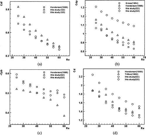
Cases listed in Table 1 are all proceeded at Re = 30. Coefficient results are achieved when it reaches “steady-state” with a convergence of 10^–4 order. G1 and G2 have the same X0, Y1, different X1 and finally almost the same results are achieved. G3 and G4 have the same X1, Y1, different X0, while their results are much different. The discrepancy of present results to the work Henderson (1995), respectively for Case G1, G2, G3, G4, C _pb is 16%, 18%, 4%, 14%, C _df is 27%, 25%, 9%, 13%, and C _dp is 14%, 14%, 5%, 15%. It is clear that the results of Case G3 are the best. In comparison with other cases (G1, G2, and G4), G3 has a longer inflow length (X0). So, it suggests that the longer inflow length the better simulation result.

Cases listed in Table 2 are all proceeded at Re = 100 with appearances of well-known Karman vortex paths. It shows that the discrepancy of the wake coefficients to the work Henderson (1995), respectively for four cases G1, G2, G3, G4, C _pb is 7%, 9%, 7%, 7%, C _df is 14%, 14%, 0%, 3%, and C _dp is 24%, 24%, 5%, 24%. Again, G3 has the lowest discrepancy of wake coefficients. Another useful characteristic parameter, vortex shedding frequency can be characterized by Strouhal number, Stg = f _q (2R)/U ₀ where f _q is the frequency of oscillation. In Table 2, Cases G1, G2, and G4 have the same Strouhal number (0.192) with a discrepancy of 16% to the experimental data (0.165) obtained by Willamson (1989) while for Case G3 the discrepancy of Strouhal number (0.172) decreases to 4%. Such conclusion can be further supported by the comparison of the larger magnitude u-component velocity at x/R = 3.24, y/R = 1.65 with the work by Braza et al. (1986). The discrepancy of the flow velocity, respectively for four cases G1, G2, G3, G4, is 16%, 16%, 5%, 16%. Therefore, it is clear that the result based on the domain of G3 is the best one compared with other domains.

Figure 2 compares present results (case G2, G3) with other works (Henderson 1995; Grove et al. 1964; Tritton 1959) at Re = 25 ∼ 60. It is clear that G3 has better results than G2. The averaged discrepancy of G3 results to other work (experimental and numerical) shown in Figure 2 is 4% while that of G2 is 17%.

FIG. 2 Coefficient versus Reynolds number: (a) C _df ; (b) C _dp ; (c) C _Pb ; (d) C _d .

To test the boundary condition v = 0 effect on the simulation results, an additional case G5 was tested. In comparison with G2, G5 has larger domain length at y-direction (Y1). The variation of the length of Y1 does not seem to have much influence on the simulation results. The comparison of G2 and G5 shows a small decrease (0.5%) of St _g when Y1 increases. This slight difference would not justify a further increase of Y1, in order to save CPU time. Therefore, it is suggested that the boundary condition v = 0 does not seem to have much influence on the simulation results.

From above analysis, it is apparent that the inflow length does an important role in determining the simulation results. Here, case G3 is found to be the best one. To study the grid effect on simulation results, case G6 and G7 were chosen with all the same parameters as case G3 except grid. The results (drag coefficient, pressure coefficient, Strouhal number, and u-component velocity) of case G6 and G7 are summarized in Table 2. It is clear that they are almost the same as those of Case G3. To save computation, we retained the coarser grid (G3) for the final computations.

Cases listed in Table 3 are all proceeded at Re = 300. With the same grids of Case G3, G6, G7 as used for Re = 100, the discrepancy of the wake coefficients to the work Henderson (1995), respectively for G3, G6, G7, C _pb is 7%, 6%, 6%, C _df is 5%, 5%, 0%, and C _dp is 9%, 8%, 8%. The discrepancies of Strouhal number to the work Williamson (1989) for the three cases G3, G6, G7 are all the same as 8%. The discrepancies of the larger magnitude u-component at x/R = 1.94, y/R = 0 to the work Braza et al. (1986), respectively, for G3, G6, G7, is 9%, 8%, and 8%. Again, the simulation results for Re = 300 are independent of the grids of G3, G6, G7. However, in comparison with the case Re = 100, the discrepancy of simulation for Re = 300 is slightly higher, which may be due to three-dimensional characteristics appearing in Re = 300 while present simulations were conducted in two-dimension. As the flow Reynolds number is larger than 188.5 (Henderson 1995), the circular cylinder wake starts having 3-dimensional characteristics. In this work, most cases' flow-Re-number is below the critical value so the flow characteristics are mostly in 2-dimension.

TABLE 3 Numerical results with different grids division at Re = 300

Cases	Elements	X1	X0	Y1	−C pb	C df	C dp	St g	u∗	h min ∗∗	h avg ∗∗
G3	50	40	−14	28	1.14	0.23	1.29	0.222	0.381	0.01	0.12
G6	60	40	−14	28	1.15	0.23	1.27	0.222	0.379	0.008	0.08
G7	80	40	−14	28	1.15	0.22	1.27	0.222	0.379	0.005	0.05
—	—	—	—	—	1.22^+	0.22^+	1.18^+	0.206^++	0.351^+++	—	—
∗ u-component larger magnitude at x/R = 1.94, y/R = 0; ∗∗ h min and h avg are the minimum and average element size in the region |R| ≤ 2; ^+ Henderson (1995), ^+ + Williamson (1989), ^+ + + Braza, Chassaing, and Minh (1986).

Flow Reynolds Number

Figure 3 shows the time-dependent evolution of the u(Figure 3a) and v-velocity components (Figure 3b). It is clear that the amplitude of u- and v-component increases with Reynolds number. Figure 3c and d shows the time-dependent evolution of the drag and lift coefficients, respectively. Again, the amplitudes of the drag and lift coefficients increase with Reynolds number. Moreover, the oscillation frequency of the wake velocity (u- and v-velocity components), drag and lift coefficient is all found to be increased due to Reynolds number increasing.

FIG. 3 Time-dependent evolution of: (a) U-component; (b) V-component; (c) drag coefficient; (d) lift coefficient (x/R = 2, y/R = 0.5).

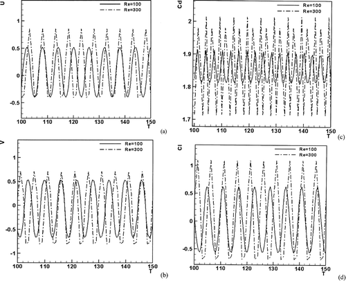
From Figure 3, it is apparent that the higher Reynolds number the higher amplitude of the wake physical properties, i.e., velocity, drag coefficient, and lift coefficient. The frequencies of these variables oscillation increase with Reynolds number and so do for vortices appearance. It is worth noting that, due to the contribution of the upper and lower alternating vortices to the drag, the frequency of the drag coefficient oscillation (shown in Figure 3c, 0.32 at Re = 100 and 0.40 at Re = 300) is twice as fast as the oscillation of the lift coefficient (shown in Figure 3d, 0.16 at Re = 100 and 0.20 at Re = 300).

Flow-Field Variable Distribution

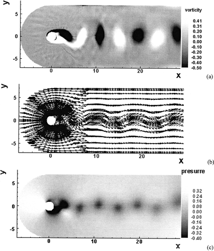
Figure 4 shows the distribution of vorticity, velocity and pressure at t = 100. It is clear that the alternating vortex patterns persist over the whole downstream distance and the vortices travel downstream through the end of the domain without any constraint. At the boundary zones between two vortex structures (vortex braid zones), the vorticity and pressure are low, but the absolute value of velocity is high. However, in the vortex core zones, the smaller velocity vector results in the higher absolute value of vorticity and higher pressure. These results are associated with the “stretching” mechanism of large-scale vortex structures in the flow field and may have an effect on the dispersion of particles.

FIG. 4 Distribution of fluid flow (Re = 100) variables at the nondimensional time of t = 100: (a) vorticity; (b) velocity; (c) pressure.

Particle Field

Particle Number Independence

To show the independence of particle number to the simulation, particle concentration function (Nrm(x) defined in Equation (13) was tested for all cases and the results are listed in Table 4. It is clear that as particle introduced number at each step is above 50, the Nrm(x) is almost constant, which is independent of particle introduced number. However, as particle introduced number is 10 or 20 at each step, the averaged particle concentration function appears slight different and the error is 2–6%. Obviously, it suggests that in this work, particle number is independent of the simulation. To save computation and obtain good presence of particle trajectory, the number of particle introduced at each step was chosen 100 for all cases.

TABLE 4 Test of particle number independence

	The number of particles introduced at each step
	10	20	50	100	200	500
	Averaged particle concentration function (Nrm(x))
St = 4, Re = 40	0.321	0.327	0.339	0.340	0.340	0.340
Re = 100	0.350	0.357	0.368	0.369	0.368	0.369
Re = 300	0.349	0.358	0.370	0.372	0.373	0.372
Re = 100, St = 0.01	0.379	0.381	0.387	0.388	0.388	0.388
St = 1	0.345	0.350	0.359	0.359	0.359	0.359
St = 10	0.341	0.349	0.354	0.354	0.354	0.354

Based on the particle tracking method introduced above, the total number of particle tracked in the whole domain was counted for each case as shown in Table 5. It is seen that the total particle number increases with the flow Re number decreasing. This is because as flow Re number decreases, flow velocity decreases leading to particle slow traveling in the flow field. In addition, in comparison with small particle, large particles tend to need more tracking in the field due to their slow traveling.

TABLE 5 Total number of particle tracked for each case

St = 4	Re =	30	40	50	60	100	300
Particle number		1091327	87646	663105	57791	29797	10457
Re = 100	St =	0.01	0.1	1	4	10	100
Particle number		28645	29157	27943	29797	35679	46789

Particle Dispersion Patterns

Flow Reynolds Number

Figure 5 shows particle instantaneous dispersion patterns (t = 100) for four particles (St = 0.01, 0.1, 1, 10) at two Reynolds numbers 100, 300. It is seen that, in the flow with a higher Reynolds number (Re = 300), particles not only disperse more in the global region but also merge interaction with vortex structures at higher level. The reason may be examined by the properties of the circular cylinder wake as analyzed above. First, with Reynolds number increasing, vortex structures spawned at higher frequency behind the circular cylinder promote particle to mix more throughout the vortex interior region. Second, as Reynolds number increases, large-scale structure of the cylinder wake stretched at higher amplitude promote particle to disperse more to the outside region of the vortex street. Therefore, it can be concluded that as flow Reynolds number increases, particle dispersion in the circular cylinder wake increases.

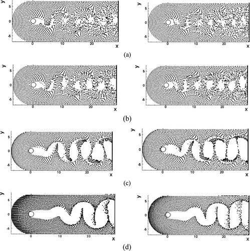
FIG. 5 Particle dispersion pattern t = 100 in the flow: Re = 100 (left), 300 (right): (a) St = 0.01, (b) 0.1, (c) 1, (d) 10.

Particle Stokes Number

Particle size (Stokes number) is one of the important factors effect on particle dispersion. In Figure 5a, small particles (St = 0.01) not only enter the core region of vortex structures but distribute in the thinned band region that connect adjacent vortex street structures. Such dispersion pattern is associated with the smaller aerodynamic response time of these particles. For the intermediate particles (St = 0.1, 1, Figure 5b and c), most of them are prevented from entering the vortex core region but are concentrated on the vortex boundaries to form highly organized distribution. This is because the aerodynamics response time of these particles is almost the same as the characteristic time scale of the wake flow. For the large particles (St = 10, Figure 5d), the dispersion of particles along the lateral direction is very little and most of the particles disperse outside of the vortex street and move toward the downstream just a slight waviness detectable in their paths. The particles are still prevented from entering the vortex core regions but the conglomeration of the particles in the boundary regions of the vortex structures becomes less, especially in the vortex braid region between two adjacent vortexes. Such pattern of particle distribution indicates that particle motion does not depend much on the vortex structure in the flow field when the Stokes number is relatively large. The reason is that the aerodynamic response time of these particles is quite longer than the characteristic time scale of the large-scale vortex structures in the flow field. Similar patterns of particle dispersion have been often observed in the gas-particle two-phase flow in the free shear flows, such as the mixing layer (Wen et al. 1992; Fan et al. 2001) and the plane wake (Tang et al. 1992; Yang et al. 2000).

Particle Dispersion Mechanism

To reveal the mechanism of the particle dispersion pattern observed in Figure 5, the relative slip velocity vector Vr, which represents the difference between the particle and fluid velocity vectors at the same time, is examined. Figure 6 shows the relative velocity vectors for different Stokes numbers at t = 100 when the flow becomes steady. When the Stokes number is small as St = 0.01 (Figure 6a), the relative slip velocity vector is fairly low (see Table 6) and distributed uniformly in the flow field, showing these particles can disperse almost as fast as the fluid. When the Stokes number is of St = 10 (Figure 6d), the relative slip velocity is at the level of O(–1) (Table 6) that is three orders higher than that of St = 0.01(O(–4)). It means that these particles slowly response to fluid motion due to large inertia effect. Subsequently, most large particles are seen (Figure 6d) to track outside of the wake street and few of them are able to reach the core region of the vortex structure.

FIG. 6 Distribution of relative velocity vector for different Stokes number at nondimensional time of t = 100 at Re = 100: (a) St = 0.01, (b) St = 0.1, (c) St = 1, (d) St = 10.

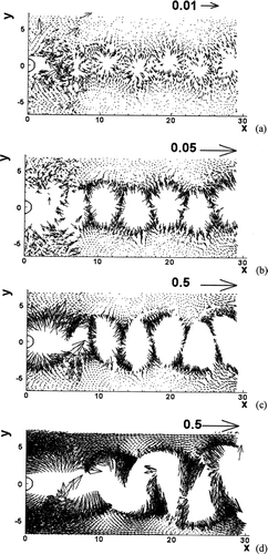
TABLE 6 Mean relative slip velocity (t = 100)

		Mean relative slip velocity
Particle St		|u − u p |	|v − v p |
0.01	Re = 100	7.033e-04	9.094e-04
0.1		5.406e-03	6.322e-03
1		2.365e-02	3.122e-02
10		1.175e-01	7.400e-02
0.01	Re = 300	6.220e-04	8.889e-04
0.1		4.868e-03	7.390e-03
1		2.322e-02	3.495e-02
10		1.093e-01	8.460e-01

However, as the Stokes numbers are intermediate, such as St = 0.1 and 1 (Figure 6b and c), the distribution of relative slip velocity vectors is extraordinary. There exist a series of saddles in the distribution of relative slip velocity vectors at the boundaries that link two opposite-sign vortex structures. In these saddles regions, the magnitude of fluid velocity is very high, but the magnitude of vorticity is quite low. The relative slip velocity vector is concentrated on the vortex braid regions that connect two roller vortex structures with opposite sign. In this case, the local focusing process of particles happens due to the folding phenomena of particles into the vortex braid regions from the adjacent vortex structures.

To make quantitative analysis of the particle size (Stokes number) and flow Reynolds number effect on particle dispersion, the mean relative slip velocity is shown in Table 6. It is clear that the value of the mean relative slip velocity increases with particle size, which is independent of the flow Reynolds number. This occurs because, as particle size increases, the ability of particle response to flow motion decreases. For all cases, the value of mean relative slip velocity at the lateral direction is higher than that at the streamwise direction, which indicates that particles disperse less along the steamwise direction and mainly follow the wake street at the lateral direction with high velocity.

It seems that the relative slip velocity vector can well reflect the dispersion mechanism of particles. From these results obtained, the dispersion patterns of particles at the intermediate Stokes numbers in the circular cylinder wake is found to be different from those in the plane mixing layers (Ling et al. 1998; Fan et al. 2001) and jets (Uthuppan et al. 1994; Aggarwal et al. 1994). The mechanism depends mostly on the strong interactions between two alternative and successive shedding vortex structures with opposite sign.

Quantitative Particle Dispersion

Particle Concentration Function

To quantify the concentration pattern of particles at the horizontal (vertical) direction, the root mean square (concentration function) of particle number per cell at x-axis (y-axis), Nrms(x) (Nrms(y)), is defined as follows:

where n _i (x) (n _i (y)) is the number of particles in the ith cell along x (y) direction.

Figure 7a and b depicts the concentration function for different flow Reynolds numbers. Along the x-direction, the profiles of Nrms(x) (Figure 7a) have several pinnacles and these pinnacles are found to just happen between two adjacent vortex structures. It indicates that such intermediate particle has high concentration between two adjacent vortex structures, which agrees well with the analysis for the dispersion pattern of particles mentioned above. As flow Reynolds number increases, the pinnacle value (Nrms(x)) shown in Figure 7a increase and the profile of the concentration function becomes more fluctuant. This is because both the amplitude and the oscillation of the flow (velocity, drag coefficient, and lift coefficient) increase with Reynolds number making more effect on particle dispersion.

FIG. 7 Particle concentration function in the flow t = 100 (a), (b) St = 4: (a) Nrms(x); (b) Nrms(y); (c), (d) Re = 100: (c) Nrms(x); (d) Nrms(y).

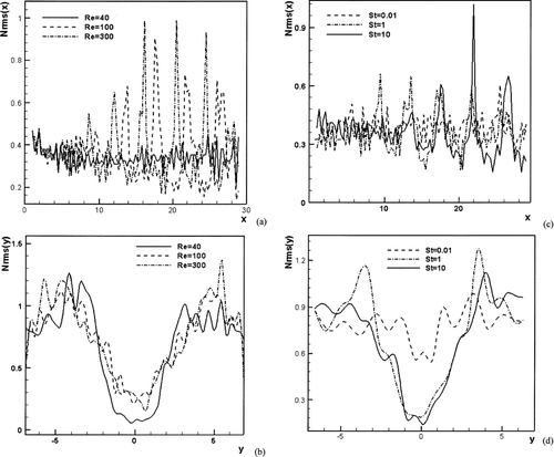
Figure 7b shows that Nrms(y) at the central region (near y = 0) is much lower than that at other regions, which is independent of the flow Reynolds number. This occurs since, most intermediate particles (St = 4) accumulate at the periphery of the large-scale structures at outside region and few of them disperse in the flow interior region. Such trend decreases with Reynolds number increasing because higher-Reynolds-number flow promotes particles to enter the flow central region. Again, as the flow Reynolds number increases, Nrms(y) increases and the profile becomes more fluctuant. This can be explained by the same reason as that for Nrms(x).

Figure 7c and d depicts the concentration function for three particles (St = 0.01, 1, 10). It is known that large-scale structures have a significant effect on the dispersion of particles, when the particle aerodynamic response time scale has the same order as the characteristic time scale of large-scale organized flow structures. Therefore, as shown in Figure 7c, the particles with the Stokes numbers of 1, 10 apparently have the larger values of Nrms(x). Corresponding to the particle concentration at the region between adjacent vortexes, there exist several pinnacles of Nrms(x) for these intermediate particles. However, as shown in Figure 7d, the value of Nrms(y) for intermediate particles (St = 1) is very low (< 0.18) near the center region (y = 0) while that for small particle (St = 0.01) is fairly high (> 0.54). On the contrast at the outside region the intermediate particles have higher Nrms(y)than the small particle does. This may be explained by the fact that small particle is able to mix with vortex structures in the center region but moderate particles tend to accumulate at the periphery of vortex structure in the outside region. Such results agree well with the analysis results mentioned above.

Particle Dispersion Function

To study the particle dispersion level due to the effect of large-scale structures quantitatively, the dispersion function of particles at the vertical (Y) direction is introduced:

where n _t is the total number of particles distributed in the whole region at time t, Y _i (t) is the particle displacement in the vertical direction at time t, and Y _m (t) is the mean value.

Figure 8a shows time-dependent particle dispersion function for particle St = 4 at the vertical direction in various flows Re = 30 ∼ 300. It is seen that the particle dispersion function increases with flow Reynolds number, especially as Re > 50 when the flow gives rising to vortex shedding with appearance of vortex street. Further, the profiles of dispersion function become more fluctuant with Reynolds number increasing. These results can be again explained by the properties of the wake flow associated with the Reynolds number. As Reynolds number increases, both the amplitude and the oscillation of the flow (velocity, drag coefficient, lift coefficient) increase and then do significant effect on particle dispersion that has been analyzed above.

FIG. 8 Time-dependent particle dispersion in the vertical direction: (a) St = 4 in various flows (Re = 30 ∼ 300); (b) different particles in the flow: Re = 100.

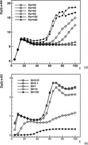
Figure 8b shows particle dispersion function for different particles (St = 0.01, 0.1, 1, 10,100) in the flow Re = 100. For particle St = 0.01, 0.1, and 1, the profile varies much with time, especially in the duration of t = 50–80 when the vortex structure is developing in progress. Due to these particles closely following with flow motion, in this period, particle dispersion function quickly increases with time and around t = 70, the value of particle dispersion function reaches the highest level. As the vortex structure shaped and shed in a normal “wake street,” particle dispersion becomes steady at an even level. In the progress of coherent structure generation, particle size plays a dominant role in particle dispersion: the smaller particle, the more particle dispersion. For particle St = 10, 100, due to their relatively large inertia, particles response to flow motion slowly and their dispersion appears much less in comparison with that of small particles. It is worth noting that the observation of particle dispersion in circular cylinder wakes appears different from that of particle dispersion in mixing layer where particle dispersion mainly depends on the progress of vortex structures rolling and pairing.

CONCLUSIONS

Numerical simulation of the two-phase flow in a flow around a cylinder was performed. The unsteady Navier-Stokes equations were solved using explicit/implicit time integration rules in time and the spectral-element method in space. The Lagrangian approach was used to trace particles based on one-way coupling. The evolution of large-scale vortex structures and the different patterns of particle dispersion in the circular cylinder wake were performed.

Based on the present simulation method, the simulation of the flow field has the averaged discrepancy to experimental work around 4%. The simulation results reveal that the amplitude of the flow physical properties (velocity, drag, and lift coefficient) increase with Reynolds number and so do the frequencies of their oscillations and vortices appearance. Due to the contribution of the upper and lower alternating vortices to the drag, the frequency of the drag coefficient oscillations is twice as fast as the oscillations of the lift coefficient.

For particle tracking, both flow Reynolds number and particle size do have a significant effect on particle dispersion. Particle dispersion increases with the flow Reynolds number and so does for particle concentration, which is independent of particle size. However, for particles at different Stokes numbers, the dispersion pattern appears much different. When the Stokes number is small as St = 0.01, particles follow the fluid flow closely and have considerable dispersion along the lateral direction. But the concentration of particles is low and their distribution is even. When the Stokes number has the order of unity, particles are observed to concentrate near the outer edges of large-scale vortex structures to form quasicoherent dispersion structures of particle. The local-focusing process of particle happens in the converging region that connects opposite sign vortex structures. So these particles are distributed very unevenly in the flow field and disperse more along the lateral direction. When the Stokes number is large as St = 10, particles tend to disperse much less along the lateral direction outside of the vortex street and move toward the downstream with even distribution.

This project is supported by the China Postdoctoral National Science Foundation (2003033539) and the National Natural Science Foundation of China (50236030).

REFERENCES

- Aggarwal , S. K. 1994 . Relationship between Stokes Number and Intrinsic Frequencies in Particle-Laden Flows . AIAA J , 32 : 1322 – 1325 .
- Brandon , D. J. and Aggarwal , S. K. 2001 . A Numerical Investigation of Particle Deposition on a Square Cylinder Placed in a Channel Flow . Aerosol. Sci. Technol. , 34 : 340 – 352 .
- Braza , M. , Chassaing , P. and Minh , H. H. 1986 . Numerical Study and Physical Analysis of the Pressure and Velocity Fields in the Near Wake of a Circular Cylinder . J. Fluid Mech. , 165 : 79 – 130 .
- Chang , E. J. and Kailasanath , K. 1996 . Simulations of Particle Dynamics in a Confined Shear Flow . AIAA J. , 34 : 1160 – 1166 .
- Chein , R. and Chung , J. N. 1988 . Simulation of Particle Dispersion in a Two-Dimensional Mixing Layer . AIChE J. , 34 : 946 – 954 .
- Crowe , C. T. , Gore , R. A. and Troutt , T. R. 1985 . Particle Dispersion by Coherent Structures in Free Shear Flows . Particul. Sci. Technol. , 3 : 149 – 158 .
- Eaton , J. K. and Fessler , J. R. 1994 . Preferential Concentration of Particles by Turbulence . Int. J. Multiphase Flow , 20 : 169 – 209 .
- Elghohashi , S. E. 1994 . On Predicting Particles by Turbulence . Applied Scientific Res. , 52 : 309 – 329 .
- Fan , J. R. , Yao , J. and Cen , K. F. 2002 . Antierosion in a 90o Bend by Particle Impaction . AIChE J , 48 : 1401 – 1412 .
- Fan , J. R. , Zheng , Y. Q. , Yao , J. and Cen , K. F. 2001 . Direct Simulation of Particle Dispersion in a Three-Dimensional Temporal Mixing Layer . Proc. R. Soc. Lond. A. , 457 : 2152 – 2166 .
- Grove , A. S. , Shair , F. H. and Petersen , E. E. 1964 . An Experimental Investigation of the Steady Separated Flow Past a Circular Cylinder . J. Fluid Mech. , 19 : 60 – 80 .
- Henderson , R. D. 1995 . Details of the Drag Curve Near the Onset of Vortex Shedding . Phys. Fluids , 7 : 2102 – 2104 .
- Ilias , S. and Douglas , P. 1989 . Inertial Impaction of Aerosol Particles on Cylinders at Intermediate and High Reynolds Numbers . Chem. Eng. Sci. , 44 : 81 – 99 .
- Korczak , K. Z. and Patera , A. T. 1986 . An Isoparametric Spectral Element Method for Solution of the Navier-Stokes Equations in Complex Geometry . J. Comput. Phys. , 62 : 361 – 382 .
- Lazaro , B. J. and Lasheras , J. C. 1992 . Particle Dispersion in the Developing Free Shear-Layer. 1. Unforced Flow . J. Fluid Mech. , 235 : 143 – 178 .
- Ling , W. , Chung , J. N. , Troutt , T. R. and Crowe , C. T. 1998 . Direct Numerical Simulation of a Three-Dimensional Temporal Mixing Layer with Particle Dispersion . J. Fluid Mech. , 358 : 61 – 85 .
- Longmire , E. K. and Eaton , J K. 1992 . Structure of a Particle-Laden Round Jet . J. Fluid Mech. , 236 : 217 – 257 .
- Richmond-Bryant , J. , Eisner , A. D. and Flynn , M. R. 2006 . Considerations for Modeling Particle Entrainment into the Wake of a Circular Cylinder . Aerosol Sci. Tech. , 40 : 17 – 26 .
- Saffman , P. G. 1965 . The Lift on a Small Sphere in a Slow Shear Flow . J. Fluid Mech. , 22 : 385 – 400 .
- Saffman , P. G. 1968 . The Lift on a Small Sphere in a Slow Shear Flow . Corrigendum , 31 : 624
- Salmanzadeh , M. , Rahnama , M. and Ahmadi , G. 2007 . Particle Transport and Deposition in a Duct Flow with a Rectangular Obstruction . Particul Sci. Technol , 25 : 401 – 412 .
- Schuh , M. J. , Schuler , C. A. and Humphrey , J. A. C. 1989 . Numerical Calculation of Particle-Laden Gas Flows Past Tubes . AIChE J. , 35 : 466 – 480 .
- Squires , K. D. and Eaton , J. K. 1991 . Measurements of Particle Dispersion Obtained from Direct Numerical Simulations of Isotropic Turbulence . J. Fluid Mech , 226 : 1 – 35 .
- Tang , L. , Wen , F. , Yang , Y. , Crowe , C. T. , Chung , J. N. and Troutt , T. R. 1992 . Self-Organizing Particle Dispersion Mechanism in a Plane Wake. . Phys. Fluids A , 4 : 2244 – 2251 .
- Tritton , D. J. 1959 . Experiments on the Flow Past a Circular Cylinder at Low Reynolds Numbers . J. Fluid Mech. , 6 : 547 – 567 .
- Uthuppan , J. , Aggarwal , S. K. , Grinstein , F. F. and Kailasanath , K. 1994 . Particle Dispersion in a Transitional Axisymmetrical Jet—A Numerical-Simulation . AIAA J , 32 : 2004 – 2014 .
- Wen , F. , Kamalu , N. , Chung , J. N. , Crowe , C. T. and Troutt , T. R. 1992 . Particle Dispersion by Vortex Structures in Plane Mixing Layers . J. Fluid Eng.—ASME. , 114 : 657 – 666 .
- Williamson , C. H. K. 1989 . Oblique and Parallel Model of Vortex Shedding in the Wake of a Cylinder at Low Reynolds Numbers . J. Fluid Mech. , 206 : 579 – 627 .
- Yang , Y. , Crowe , C. T. , Chung , J. N. and Troutt , T. R. 2000 . Experiments on Particle Dispersion in a Plane Wake . Int. J. Multiphase Flow , 26 : 1583 – 1607 .
- Yao , J. 2002 . Direct Numerical Simulation of Particle Dispersion in the Temporal Wake of a Circular Cylinder & Numerical Investigation of a New Method for Protecting Bends from Erosion in Gas-particle Flows Ph.D. dissertation, Zhejiang University
- Yao , J. , Ji , F. , Liu , L. , Fan , J. R. and Cen , K. F. 2003 . Direct Numerical Simulation of the Particle Flow in the Wake of Circular Cylinder . Prog. Nat. Sci. , 13 : 379 – 384 .
- Yao , J. , Zhang , B. Z. and Fan , J. R. 2000 . An Experimental Investigation of a New Method for Protecting Bends from Erosion in Gas-Particle Flows . Wear , 240 : 215 – 222 .
- Zhang , X. Y. and Ahmadi , G. 2005 . Eulerian-Lagrangian Simulation of Liquid-Gas-Solid Flows in Three-Phase Slurry Reactors . Chem. Eng. Sci. , 60 : 5089 – 5104 .