Satellite Remote Sensing for Developing Time and Space Resolved Estimates of Ambient Particulate in Cleveland, OH

Abstract

This article empirically demonstrates the use of fine resolution satellite-based aerosol optical depth (AOD) to develop time and space resolved estimates of ambient particulate matter (PM) ≤2.5 μm and ≤10 μm in aerodynamic diameters (PM_2.5 and PM₁₀, respectively). AOD was computed at three different spatial resolutions, i.e., 2 km (means 2 km × 2 km area at nadir), 5 km, and 10 km, by using the data from MODerate Resolution Imaging Spectroradiometer (MODIS), aboard the Terra and Aqua satellites. Multiresolution AOD from MODIS (AOD_MODIS) was compared with the in situ measurements of AOD by NASA's AErosol RObotic NETwork (AERONET) sunphotometer (AOD_AERONET) at Bondville, IL, to demonstrate the advantages of the fine resolution AOD_MODIS over the 10-km AOD_MODIS, especially for air quality prediction. An instrumental regression that corrects AOD_MODIS for meteorological conditions was used for developing a PM predictive model.

The 2-km AOD_MODIS aggregated within 0.025° and 15-min intervals shows the best association with the in situ measurements of AOD_AERONET. The 2-km AOD_MODIS seems more promising to estimate time and space resolved estimates of ambient PM than the 10-km AOD_MODIS, because of better location precision and a significantly greater number of data points across geographic space and time. Utilizing the collocated AOD_MODIS and PM data in Cleveland, OH, a regression model was developed for predicting PM for all AOD_MODIS data points. Our analysis suggests that the slope of the 2-km AOD_MODIS (instrumented on meteorological conditions) is close to unity with the PM monitored on the ground. These results should be interpreted with caution, because the slope of AOD_MODIS ranges from 0.52 to 1.72 in the site-specific models. In the cross validation of the overall model, the root mean square error (RMSE) of PM₁₀ was smaller (2.04 μg/m³ in overall model) than that of PM_2.5 (2.5 μg/m³). The predicted PM in the AOD_MODIS data (∼2.34 million data points) was utilized to develop a systematic grid of daily PM at 5-km spatial resolution with the aid of spatiotemporal Kriging.

1. INTRODUCTION

During the last decade, satellite remote sensing has advanced substantially, especially after the launch of the Earth Observing System (EOS) satellite in December 1999. Several sensors, aboard many sun-synchronous and geostationary satellites, have been orbiting the earth and recording data in many different spectral bands and at many spatial resolution and temporal intervals. In recent years, researchers are increasingly using these data to estimate aerosol optical depth (AOD) for climate change studies. Because AOD can help assess time–space dynamics of radiative forcing that plays an important role in climate change studies. The recent literature also suggests that AOD has a great potential to develop time and space resolved estimates of air quality (Chu et al. 2003; Gupta et al. 2006; Kumar 2010b; van Donkelaar et al. 2010). Because spatiotemporal coverage of in situ air pollution monitoring worldwide is very limited, these estimates are critically important for air quality surveillance and management and epidemiological studies. For example, there are only two operational stations in the City of Chicago that record ambient particulates ≤10 μm in aerodynamic diameter (PM₁₀). These two stations alone are unlikely to gather data that can adequately represent population exposure to ambient PM₁₀.

In this article, we demonstrate the use of high-resolution AOD to develop time and space resolved estimates of airborne particulates ≤2.5 μm, ≤10 μm, and >2.5 μm and ≤10 μm in aerodynamic diameters (PM_2.5, PM₁₀, and PM_10–2.5) in the Cleveland Metropolitan Statistical Area (MSA) from 2000 to 2009. A dozen recent studies have investigated the use of satellite-based AOD to predict ambient particulate matter (PM) of different sizes (Wang and Christopher 2003; Gupta et al. 2006; Kumar et al. 2007, 2008; Martin 2008; Gupta and Christopher 2009a; Hoff and Christopher 2009; Liu et al. 2009; van Donkelaar et al. 2010). Despite this, our understanding of how to predict time and space resolved estimates of ambient PM is far from complete, because the AOD–PM association is not straightforward for several reasons. First, AOD retrieval using satellite data is not a direct measurement and has inherent uncertainties due to the assumptions of the radiative forcing model. In addition, several factors can influence the robustness of AOD, such as cloud contamination, surface glint, types of aerosols, and spatial resolution at which AOD is computed and aggregated (Li et al. 2005; Zhang and Reid 2006; Kumar 2010b). Therefore, the quality of the predicted PM is dictated by the robustness of AOD. Second, the concentration of ambient PM varies significantly within a short distance (Kumar et al. 2007). Thus, the coarse spatial resolution of AOD, such as the 10-km AOD extensively used by researchers (Gupta and Christopher 2009a; Liu et al. 2009), is unlikely to capture microenvironment variability of ambient PM. Third, there are subtle differences in the spatial, temporal, and vertical scales at which AOD and PM data are collected, aggregated, and made available to researchers. Thus, the spatiotemporal scales used to collocate and aggregate these data can influence the degree of generalization and hence the AOD–PM association. The satellite-based AOD is a columnar estimate that represents a fraction of a minute's time over an area on a given day. PM data, however, are point measurements recorded at sparsely distributed locations on the ground at different time intervals—every hour, 8 h, or 24 h. Unlike AOD, which consists of airborne solid and liquid aerosols, PM is just the dry mass. AOD represents three distinct types of aerosols: aerosols generated by human activities (AOD_h), aerosols generated by natural processes (AOD_n), and aerosols generated through the interaction of AOD_h with AOD_n. Among these, AOD_h that consists of airborne dry mass is likely to show a stronger association with PM except for arid and semiarid areas and areas with frequent dust storm, because fine dust can also account for dry PM mass. But if the AOD_n component dominates, it is likely to result in a weak association between AOD and PM. Therefore, failing to account for AOD_n and AOD_n ∩ AOD_h can result in a weak AOD–PM association. Fourth, nature and sources of aerosols and meteorological and climatic conditions vary regionally and play important roles in AOD retrieval and its association with PM. This means that the AOD–PM association observed in one region may not be extrapolated to other regions. Therefore, it is important to examine how regional factors can influence the AOD–PM association.

This article demonstrates how the high resolution (2-km AOD_MODIS) can improve the robustness of AOD and help address indirectly most of the above concerns that hinder our ability to develop the ambient concentration of PM by using AOD_MODIS and ancillary data. In particular, this article has two objectives. First, it examines how the robustness of satellite-derived AOD changes with respect to the spatial resolution of AOD retrieval and spatiotemporal scales used for aggregating AOD. Second, utilizing the 2-km AOD_MODIS and PM data (from Environmental Protection Agency [EPA]), it develops an empirical model to estimate ambient PM. To demonstrate the application of this model, daily PM_2.5, PM₁₀, and PM_10–2.5 concentrations were computed in Cleveland and surrounding areas from 2000 to 2009. The remainder of this article describes the data and methods used for the analysis, presents the results of the analysis, and provides a detailed discussion on the finding of this article with the relevant literature.

2. METHODOLOGY

2.1 Data

Data for this research come from four different sources, namely, MODIS Level 1 and Level 2 data from NASA (2010), AERONET data from NASA (2007), meteorological data from the National Climatic Data Center (NCDC 2007), and PM data from EPA (2008). All these datasets were available with the GMT time stamp and location coordinates, which made the temporal comparison and integration possible. These data are described in the following sections.

2.1.1. MODIS Data

Terra and Aqua satellites (that have MODIS aboard) were launched on December 18, 1999, and May 4, 2002, respectively, and MODIS data have been available since February 24, 2000, and June 24, 2002, respectively. MODIS records spectral radiances in 36 bands, which can be grouped by three different spatial resolutions: 0.25, 0.5, and 1.0 km. To extract AOD_MODIS, we acquired the following MODIS datasets through December 2009 from both satellites: Level 1b calibrated radiances—1.0 km, Level 1b calibrated radiances—0.5 km, Level 1b calibrated radiances—0.25 km, geolocation—1.0 km, Level 2 join atmospheric products of profiles, total column ozone, water vapor, and stability indices, and Level 2 cloud mask and spectral test results.

2.1.2. AERONET Data

In situ hourly AOD_AERONET data were downloaded from NASA's Web site for Bondville, IL (NASA 2007). AOD_AERONET was computed at 0.550 μm to match the spectral resolution of AOD_MODIS. These data were used to compare the robustness of multiresolution AOD_MODIS. The level 2.0 AERONET data used in this research were screened for cloud contamination by using the methodology of Smirnov et al. (2000).

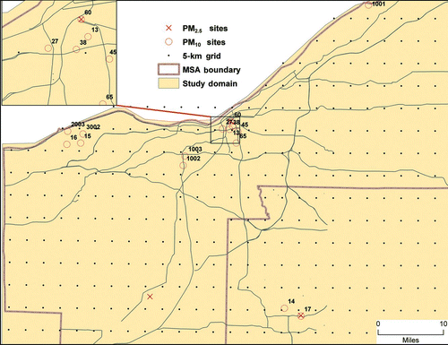
FIG. 1 Study area—Cleveland metropolitan statistical area and PM_2.5 and PM₁₀ monitoring stations. (Figure available in color online.)

2.1.3. NCDC Data

Global surface hourly data on meteorological conditions, including relative humidity, surface temperature, wind direction, wind speed, dew point, and atmospheric pressure, were acquired from NCDC. These data were critically important for developing the AOD-PM empirical model, because meteorological conditions can influence AOD_MODIS greatly. For example, the value of AOD_MODIS increases with the increase in relative humidity, because not only does it increase the concentration of water vapors, but it also inflates particle size (Ramachandran 2007). Other factors, such as wind speed and atmospheric pressure, can influence aerosols mixing within the boundary layer height (Tripathi et al. 2007; Gupta and Christopher 2009b). This, in turn, also influences uncertainty in AOD_MODIS retrieval.

2.1.4. EPA Data

PM₁₀ and PM_2.5 data from 2000 to 2009 were acquired from EPA from all monitoring stations in the Cleveland MSA and surrounding areas (EPA 2008; Figure 1). These data were needed to develop and validate an empirical PM-AOD_MODIS model. Although there were many monitoring stations, data from five PM_2.5 and three PM₁₀ monitoring stations were used, because the data from only these stations had adequate number of data points within the optimal 0.025° distance and 60-min time intervals of AOD_MODIS data.

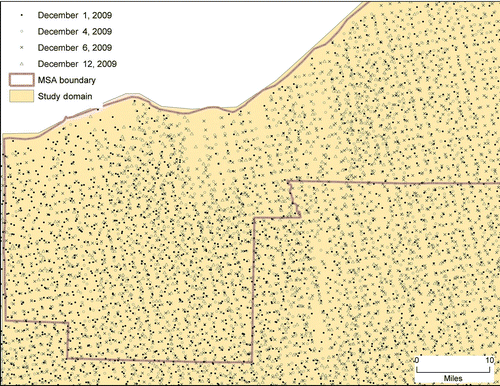
FIG. 2 Location of AOD and imputed PM₁₀, PM_2.5, and PMC values in the first 2 weeks of December 2009. (Figure available in color online.)

2.2 Methods

2.2.1 Data Integration

The data for this research were acquired from multiple sources and these data were available at different spatiotemporal scales. The multiresolution AOD_MODIS (2, 5, and 10 km) was collocated with the AOD_AERONET data (at Bondville, IL) within 3 h time and 0.6° distance intervals, and were averaged within different time and distance intervals to demonstrate how uncertainty in AOD_MODIS changes with respect to the change in time and distance intervals used for aggregating these data.

AOD_MODIS was collocated with the hourly PM data monitored on the ground at sparsely distributed monitoring stations in the study area (Figure 1). Let y_ith denotes PM observed at sites ; for hours h = 1, …, H; and days t = 1, …, T. Since AOD_MODIS locations are distributed sporadically and do not correspond with the PM monitoring sites (Figure 2), AOD_MODISlocations are distinguished from y_ith sites. Let τ_atp denotes AOD_MODIS at locations a = 1, …, A; days t = 1, …, T; and satellite overpass time (or hour of AOD_MODIS) p = 1, …P. On a given day, τ_atp can be observed at multiple locations (a) around the ith site. Likewise, the overpass (or recording) time (p) of AOD_MODIS does not correspond with the duration and time (h) of y_ith on the same day. Consequently, there can be many AOD_MODIS values around the ith site on a given day, but one value within an hour interval between the time of PM observation and AOD_MODIS data. The τ_atp data were aggregated to match the spatiotemporal resolutions of PM data. AOD_MODIS, comparable with the PM data (τ_ith ), within a given distance interval around the ith site with distance (d_ia ) and time difference (m_hp ) between AOD_MODIS and y_ith was computed as

where ω is 1 if the distance between ath location (i.e., centroid of an AOD pixel) and ith site ≤ d_ia and the difference between pth time of AOD_MODIS and hth recording time of PM at ≤ m_hp (for m_hp = 15, 30, …, 180 min), or 0 otherwise.

A similar procedure was adopted to collocate AOD_MODIS with the AOD_AERONET data; the collocated data were restricted with 3-h time and 0.6° distance intervals.

2.2.2 Statistical Methods

Descriptive statistics and correlation were used for the exploratory analysis, and instrumental regression was employed to develop a PM predictive model. Further, we employed a cross-validation method to evaluate the performance of the regression models. An empirical relationship between AOD_MODIS and PM (observed at the existing EPA sites) was developed, and then this relationship was applied for all data points in the 2-km AOD_MODIS dataset to predict PM. Since both AOD_MODIS and PM observed a highly skewed distribution, both were transformed to log scales for the analysis. As described earlier, AOD_MODIS is a columnar measurement and can be greatly influenced by meteorological conditions. Instrumenting AOD_MODIS on meteorological conditions can help overcome this problem, as

where ϕ is the regression coefficient and M′ _t is a design matrix of meteorological variables, including temperature, wind direction, wind velocity, and atmospheric pressure. As we are using surface measurement and there are limited numbers of monitoring stations, we assume meteorological conditions to be the same within the study area at the crossing time of Terra and Aqua satellites (i.e., time stamp on the AOD_MODIS). For example, wind direction is likely to be the same at tth time (on a given day) within the Cleveland MSA. To control for intratime and intracity structure, time (ν_t ) and site (s_i ) specific fixed effects can be introduced in Equation (2), as

Since both AOD_MODIS and PM data showed a strong temporal and seasonal structure, Equation (3) was extended to control for temporal and seasonal structure as

where C_t is the month number since January 2000 (January 2000 = 1 and December 2009 = 120) and controls for cyclic trend; S_it is a seasonal dummy (1 = summer, 0 otherwise). Solving Equation (4) can allow us to estimate for each data point τ_atp in the AOD_MODIS dataset. This, however, does not ensure an estimate of for any point location and time within the study domain, because of missing values in the AOD_MODIS dataset due to cloud cover and mismatches in the location and time of AOD_MODIS and other datasets. We suggest the use of spatiotemporal Kriging to impute PM for any given location and time by using the predicted values () in the AOD_MODIS dataset as it minimizes prediction error (De Iaco et al. 2002). We have developed a software application in C++ to implement spatiotemporal Kriging: this application takes the predicted values () and imputes it () for any location (j) and time (T). In this research, daily PM_2.5, PM₁₀, and PM_10–2.5 were developed for a 5-km grid overlaid onto the Cleveland MSA from 2000 to 2009; the results of the analysis and imputation are discussed in the next section.

2.2.3 Procedure for Extracting Multiresolution AOD

We retrieved the 10-km AOD_MODIS at 0.550 μm over land by using the algorithm employed for AOD_MODIS in the Collection 5.0 (Levy et al. 2007). The MODIS spectral channels used in retrieving AOD over land and ocean included two 0.25 km (0.660 and 0.860 μm) channels and five 0.5 km (0.470, 0.550, 1.240, 1.640, and 2.130 μm) channels. The 0.25-km resolution (0.660 and 0.860 μm) channels were used to detect water bodies, such as lakes and rivers. The detailed procedures of screening clouds and surface snow/ice and computing AOD_MODIS using MODIS data are discussed elsewhere (Remer et al. 2006). At the final step, pixels that passed screening tests were further analyzed for computing AOD_MODIS. For the 10-km AOD_MODIS, for example, pixels were selected within a range of 20th–50th percentile of reflectances in ascending order that removes the upper 50% and the lower 20% of the pixels to avoid the possible subpixel contamination by clouds, surface snow/ice, and water bodies. The algorithm (used for the Collection 5.0) requires at least 12 pixels in order to compute an AOD_MODIS value for a pixel. Otherwise, a missing (−9999) is attached to the pixel.

We employed the same algorithm to retrieve the 2- and 5-km AOD_MODIS as used by NASA for retrieving the 10-km AOD_MODIS in the Collection 5.0 (Levy et al. 2007). The only differences are in the final stage of the algorithm for selecting the minimum number of pixels required for a valid AOD_MODIS retrieval. For the 10-km AOD_MODIS, the minimum number of valid pixels required is 12 out of a total of 400 available pixels. Since the number of pixels available within 5 × 5 km area and 2 × 2 km area was reduced to 1/4 and 1/25, the degree of freedom to select the best pixels was also reduced significantly. If we reduce the number of pixels in proportion to reduction in the area, we will be left with only 3 and 0.5 pixels for the 5- and 2-km AOD_MODIS, respectively. Since this number is very small and can result in greater uncertainty, we doubled this number and set 5 pixels as the minimum threshold for computing the 5-km AOD_MODIS and 2 pixels for the 2-km AOD_MODIS.

In the 10-km AOD_MODIS algorithm, we arrange reflectance values in ascending order and eliminate the top 50% brighter pixels due to cirrus or subpixel cloud contamination and 20% darker pixels due to snow/ice and water bodies. We maintain the same quality for selecting the best 30% pixels within the range of 20th–50th percentiles of reflectance values for the 2- and 5-km AOD_MODIS. Of the screened pixels (between 20 and 50 percentiles of reflectance values), the minimum number of valid pixels required was reduced to 5 and 2 for the 5- and 2-km AOD_MODIS, respectively. In terms of percentage, these values were 17% and 40% for the 5- and 2-km AOD_MODIS, respectively. This is a more restrictive criterion for the selection of the minimum number of pixels required to compute AOD_MODIS as compared with that used for the 10-km AOD_MODIS, i.e., 10%. Therefore, the 2- and 5-km AOD_MODIS are likely to be more robust than the 10-km AOD_MODIS.

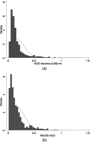
FIG. 3 (a) Statistical distribution of AOD_ANet at Bondville, IL, 2000–2007. (b) Statistical distribution of the 2-km AOD_MODIS, aggregated within 0.15° and 1-h intervals of AOD_ANet data at Bondville, IL, 2000–2007.

3. RESULTS

3.1. A Comparison of Multiresolution AOD_MODIS and Its Aggregation Across Spatiotemporal

The 8-year average of AOD_AERONET at Bondville, IL, was 0.1601 ± 0.0006 (Table 1). Both multiresolution 2-, 5-, and 10-km AOD_MODIS and AOD_AERONET recorded a positively skewed distribution (Figures 3a and b). This suggests that the events of high-aerosol loading occurred for only a limited number of days during these 8 years. The differences between AOD_AERONET and AOD_MODIS (at 2-, 5-, and 10-km spatial resolutions) were not large. However, these differences were statistically significant. Since AOD_AERONET and AOD_MODIS record the same thing (i.e., AOD), the fundamental question is why the averages of AOD_AERONET and AOD_MODIS are significantly different? The differences in the values of AOD_AERONET and AOD_MODIS can arise due to two important reasons: differences in the methodology for computing AOD and differences in the spatial and temporal scales of these datasets.

TABLE 1 Descriptive statistics of AOD_MODIS and AOD_ANet, at Bondville, IL (2000–2007)

	MODIS AOD				Aeronet AOD 0.550 μm
Spatial resolution (km)	Mean	Median	95% CI	N	Mean	Median	95% CI	N
2	0.151	0.092	0.0050	4235	0.1608	0.1049	0.0006	14,003
5	0.168	0.106	0.0065	3095
10	0.153	0.097	0.0068	2034
Note: AOD retrieval was restricted with 0.05° of Aeronet stations.

AOD_ARONET is a direct measurement recorded by a sunphotometer (NASA 2007). However, AOD_MODIS is an area measurement (such as 2, 5, and 10 km) computed using the same aerosol retrieval algorithm with radiative-transfer-model-generated lookup tables (Remer et al. 2005, 2006; Levy et al. 2007). AOD_MODIS represents the AOD concentration for a fraction of a minute when a satellite is over an area, and the AOD_AERONET data are aggregated hourly at the point location of the sunphotometer. Since AOD_MODIS computation using radiative transfer models is based on many assumptions about aerosol and surface properties (Chu et al. 2003), AOD_MODIS often suffers from uncertainties in association with the assumed aerosol properties and surface characteristics. Over the eastern US, the assumption of dark surface is generally valid (Chu et al. 2003) except in the urban areas. Furthermore, the degree of uncertainty increases as the spatial resolution of AOD_MODIS retrieval increases as demonstrated by Kumar et al. (2008).

The robustness of AOD_MODIS is evaluated by comparing it with the in situ measurements of AOD_AERONET by the sunphotometer (Chu et al. 2002; Ichoku et al. 2002; Li et al. 2005) for two important reasons. First, the sunphotometer measures AOD directly (without assuming a particular aerosol model), and data on the variables that can bias the AOD value are recorded at the AERONET stations such as angstrom exponent. Therefore, the estimation and calibration of AOD_AERONET are more reliable (Dubovik et al. 2000). For AOD_MODIS, however, the spectral reflectance (especially bright surfaces) can bias AOD_MODIS upward or downward. Second, despite the mismatch in the spatial scale and spatiotemporal intervals of aggregation, both AOD_MODIS and AOD_AERONET show a very strong spatiotemporal autocorrelation, due to the longer (about a week) lifetime of aerosols and their significant movement across geographic spatiotemporal.

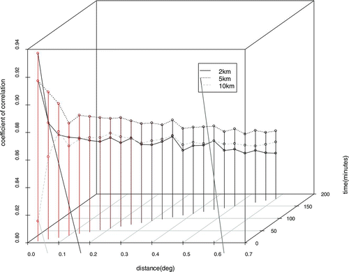
FIG. 4 Association between multiresolution (2, 5, and 10 km) AOD_MODIS and AOD_ANet at different spatiotemporal intervals in Bondville, IL, 2000–2007. (Figure available in color online.)

Despite these two reasons, these two datasets are not fully comparable, because the computation method and spatial resolution of AOD_MODIS and AOD_AERONET are subtly different and the differences between AOD_MODIS and AOD_AERONET should not be surprising. When the spatiotemporal resolution of these two datasets is the same, the coefficient of correlation between them must ∼1 and the deviation of this correlation from unity is most likely attributed to uncertainty in AOD_MODIS retrieval.

The 2-, 5-, and 10-km AOD_MODIS, aggregated at different spatiotemporal intervals, were correlated with the AOD_AERONET. Table 2 and Figure 4 show how the correlation between AOD_AERONET and the 2- and 5-km AOD_MODIS drops gradually with the increasing spatiotemporal intervals used for aggregating these data. For the 10-km AOD_MODIS, however, correlations were in the range of 0.73–0.77 within 0.05° distance (because of very few data points), but it improved to 0.88 when the distance interval increased to 0.075 distance and 15-min time intervals. This pair of distance and time intervals only depicts the correlation that is a maximum in our time and space domains. It could vary across different increments of space and time. Therefore, it should be more important to note that the correlation between AOD_AERONET and AOD_MODIS was ≥0.83 for distance ≥0.05 regardless of the time interval. It is worth noting that the correlation value was ∼0.92 for the 2-km AOD_MODIS when these data were aggregated within 0.025° and 15-min time intervals.

TABLE 2 The coefficient of correlation between AOD_MODIS and AOD_ANet at 550 nm, Bondville, IL (2000–2007)

	Spatial resolution
	2 km				5 km				10 km
	Time difference between Aeronet AOD and MODIS AOD recording (min)
Distance (deg)	15	30	60	120	15	30	60	120	15	30	60	120
0.025	0.918 (179)	0.913 (341)	0.910 (672)	0.882 (1265)	0.910 (94)	0.892 (177)	0.874 (324)	0.851 (604)	0.771 (53)	0.761 (110)	0.731 (210)	0.741 (380)
0.050	0.884 (456)	0.891 (882)	0.890 (1724)	0.858 (3220)	0.907 (338)	0.899 (672)	0.890 (1299)	0.868 (2399)	0.860 (207)	0.855 (433)	0.851 (857)	0.837 (1590)
0.075	0.867 (793)	0.877 (1534)	0.877 (2992)	0.847 (5588)	0.889 (642)	0.889 (1289)	0.884 (2509)	0.863 (4627)	0.878 (436)	0.872 (898)	0.863 (1791)	0.839 (3340)
0.100	0.859 (1171)	0.871 (2278)	0.870 (4449)	0.845 (8299)	0.879 (1003)	0.881 (2009)	0.875 (3931)	0.855 (7277)	0.864 (780)	0.865 (1596)	0.855 (3165)	0.834 (5882)
0.125	0.858 (1571)	0.869 (3070)	0.869 (6009)	0.844 (11,231)	0.881 (1429)	0.883 (2859)	0.877 (5603)	0.859 (10,376)	0.863 (1166)	0.867 (2372)	0.862 (4681)	0.840 (8674)
0.150	0.852 (1748)	0.869 (3424)	0.868 (6710)	0.840 (12,531)	0.885 (1673)	0.888 (3351)	0.881 (6577)	0.861 (12,148)	0.865 (1402)	0.870 (2864)	0.863 (5658)	0.842 (10,469)
0.175	0.854 (2017)	0.866 (3949)	0.867 (7739)	0.843 (14,484)	0.884 (1963)	0.887 (3943)	0.880 (7741)	0.860 (14,338)	0.866 (1744)	0.870 (3538)	0.867 (6964)	0.848 (12,919)
0.200	0.857 (2199)	0.866 (4308)	0.866 (8441)	0.842 (15,822)	0.882 (2241)	0.885 (4508)	0.879 (8872)	0.860 (16,448)	0.869 (2052)	0.874 (4170)	0.869 (8222)	0.849 (15,237)
0.225	0.854 (2449)	0.866 (4807)	0.867 (9429)	0.844 (17,680)	0.884 (2524)	0.888 (5094)	0.881 (10,026)	0.864 (18,589)	0.870 (2355)	0.875 (4784)	0.870 (9448)	0.852 (17,571)
0.250	0.854 (2872)	0.866 (5646)	0.868 (11,077)	0.847 (20,779)	0.885 (2988)	0.889 (6040)	0.882 (11,903)	0.864 (22,079)	0.872 (2873)	0.875 (5844)	0.871 (11,539)	0.854 (21,456)
0.275	0.854 (3303)	0.866 (6504)	0.869 (12,766)	0.848 (23,977)	0.883 (3490)	0.888 (7063)	0.882 (13,925)	0.863 (25,849)	0.868 (3418)	0.874 (6957)	0.870 (13,763)	0.853 (25,618)
0.300	0.851 (3491)	0.864 (6872)	0.867 (13,479)	0.845 (25,303)	0.883 (3738)	0.889 (7571)	0.881 (14,960)	0.864 (27,795)	0.866 (3715)	0.873 (7566)	0.870 (14,996)	0.853 (27,919)
0.325	0.852 (3747)	0.865 (7388)	0.868 (14,506)	0.847 (27,273)	0.882 (4091)	0.888 (8280)	0.881 (16,346)	0.863 (30,382)	0.867 (4071)	0.874 (8292)	0.870 (16,431)	0.855 (30,647)
0.350	0.851 (4176)	0.865 (8242)	0.868 (16,195)	0.848 (30,497)	0.881 (4646)	0.888 (9402)	0.881 (18,577)	0.864 (34,578)	0.864 (4624)	0.872 (9430)	0.869 (18,725)	0.855 (34,946)
0.375	0.851 (4619)	0.865 (9124)	0.869 (17,943)	0.849 (33,829)	0.880 (5197)	0.888 (10,534)	0.881 (20,830)	0.863 (38,787)	0.863 (5226)	0.872 (10,669)	0.867 (21,178)	0.852 (39,515)
0.400	0.850 (5069)	0.865 (10,019)	0.869 (19,708)	0.849 (37,209)	0.879 (5793)	0.887 (11,746)	0.880 (23,240)	0.862 (43,315)	0.863 (5848)	0.872 (11,941)	0.867 (23,706)	0.851 (44,246)
0.425	0.850 (5249)	0.865 (10,365)	0.869 (20,394)	0.849 (38,503)	0.879 (6109)	0.887 (12,392)	0.880 (24,513)	0.863 (45,713)	0.862 (6191)	0.871 (12,627)	0.866 (25,085)	0.852 (46,876)
0.450	0.849 (5547)	0.864 (10,970)	0.868 (21,575)	0.848 (40,789)	0.878 (6474)	0.886 (13,146)	0.879 (26,011)	0.862 (48,532)	0.861 (6582)	0.871 (13,445)	0.866 (26,706)	0.851 (49,910)
0.475	0.847 (6023)	0.863 (11,922)	0.867 (23,443)	0.848 (44,387)	0.877 (7102)	0.886 (14,429)	0.879 (28,566)	0.862 (53,347)	0.860 (7247)	0.871 (14,815)	0.866 (29,439)	0.852 (55,055)
0.500	0.844 (6215)	0.860 (12,301)	0.866 (24,197)	0.846 (45,817)	0.877 (7436)	0.886 (15,120)	0.878 (29,933)	0.863 (55,878)	0.860 (7661)	0.871 (15,651)	0.865 (31,117)	0.851 (58,234)
0.525	0.846 (6515)	0.862 (12,906)	0.867 (25,383)	0.848 (48,131)	0.875 (7818)	0.884 (15,906)	0.878 (31,504)	0.862 (58,913)	0.860 (8038)	0.871 (16,439)	0.866 (32,684)	0.852 (61,192)
0.550	0.845 (6705)	0.862 (13,277)	0.867 (26,127)	0.848 (49,567)	0.876 (8164)	0.885 (16,641)	0.879 (32,986)	0.863 (61,706)	0.858 (8426)	0.869 (17,242)	0.864 (34,318)	0.849 (64,262)
0.575	0.843 (7013)	0.860 (13,910)	0.866 (27,363)	0.847 (51,963)	0.874 (8561)	0.883 (17,430)	0.877 (34,546)	0.861 (64,669)	0.858 (8868)	0.870 (18,146)	0.865 (36,106)	0.851 (67,656)
0.600	0.840 (7513)	0.859 (14,915)	0.864 (29,355)	0.846 (55,803)	0.871 (9286)	0.881 (18,921)	0.876 (37,530)	0.860 (70,313)	0.856 (9654)	0.868 (19,746)	0.864 (39,296)	0.851 (73,661)

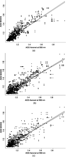
From this analysis, two important findings emerge. First, the 2-km AOD_MODIS, aggregated within the finest spatiotemporal intervals, recorded the best association (∼0.92) with the AOD_AERONET, despite the fact that the overall correlation value does not drop below 0.73 for any spatiotemporal intervals, and for any spatial resolution of AOD_MODIS. This finding suggests that a major fraction of AOD_MODIS (that consists of aerosols generated through natural processes, such as water vapors and dust) exhibits a strong spatiotemporal autocorrelation. Therefore, the correlation between AOD_AERONET and AOD_MODIS is strong and positive even within 0.6° (∼52 km at Bondville) and 120-min time intervals. Second, we begin to lose details about a small fraction of AOD_MODIS that consists of aerosols generated through anthropogenic sources (such as emission from point and mobile sources) as the spatiotemporal intervals used for aggregation and the spatial resolution of AOD_MODIS retrieval become coarser. As evident from Figure 5, there is a one-to-one correspondence between AOD_MODIS and AOD_AERONET data at the 2-km spatial resolution at the fitted line, and the extent of scattering (around the line of best fit) increases significantly for the 5- and 10-km AOD_MODIS. Therefore, we suggest the use of 2-km AOD_MODIS for developing air quality estimates. Not only do these data ensure better locational precision, but also have a significantly large number of data points, which is critically important for imputing systematic spatiotemporal grids of air pollution exposure with the minimal uncertainty.

FIG. 5 (a) Association between the 2-km AOD_MODIS and AOD_ANet in Bondville, IL, 2000–2007. (b) Association between the 5-km AOD_MODIS and AOD_ANet in Bondville, IL, 2000–2007. (c) Association between the 10-km AOD_MODIS and AOD_ANet in Bondville, IL, 2000–2007.

3.2. Spatial Distribution of PM and AOD_MODIS

PM data are monitored at sparsely located sites (Figure 1), and the locations of daily AOD_MODIS (irrespective of the spatial resolution of their retrieval) vary significantly (Figure 2), and the same location repeats every 16th day. Although there were many sites where PM data were monitored, the hourly PM_2.5 and PM₁₀ data that corresponded with the time intervals of Terra and Aqua satellites (i.e., 9 a.m. to 3 p.m. local time) were available for five and four sites, respectively. Both PM₁₀ and PM_2.5 recorded a significant spatial variation in the annual averages (Tables 3 and 4): PM₁₀ concentration ranged from 18.0 to 41.4 μg/m³, and PM_2.5 concentration ranged from as low as 10.5 μg/m³ at a suburban site to as high as 16.0 μg/m³ at the downtown site. Since there were subtle differences in the spatiotemporal scales of PM and AOD_MODIS data, these data were aggregated using optimal spatial (0.025° distance interval at nadir, i.e., spatial interval at which AOD_MODIS recorded the best association with AOD_AERONET) and 1-h time intervals (because that was the finest temporal scale at which PM data were available).

TABLE 3 PM_2.5 monitoring stations in Cleveland, OH

Site no.	Longitude (deg)	Latitude (deg)	μg/m^3	Beginning year	Ending year
3	−81.9117	41.10278	16.1 ± 0.11	2005	2009
7	−80.7875	41.21417	13.1 ± 0.11	2005	2009
17	−81.4686	41.06333	14.1 ± 0.10	2002	2009
20	−81.3733	40.80056	10.5 ± 0.07	2002	2009
60	−81.6785	41.49395	16.0 ± 0.13	2002	2009
3002	−81.7005	41.58614	12.5 ± 0.08	2004	2009
Total	−81.5079	41.20068	13.3 ± 0.04	NA

TABLE 4 PM₁₀ monitoring stations

Site no.	Longitude (deg)	Latitude (deg)	μg/m^3	Beginning year	Ending year
5	−80.8019	41.2308	19.7 ± 0.86	2000	2009
6	−80.8106	41.2019	19.5 ± 0.83	2000	2009
7	−80.7875	41.2142	19.1 ± 0.89	2000	2008
9	−81.3347	40.8183	23.1 ± 1.61	2000	2004
13	−81.6733	41.4842	41.4 ± 1.22	2000	2003
14	−81.5167	41.0792	20.1 ± 0.12	2000	2005
15	−82.1208	41.4428	21.5 ± 1.76	2000	2001
16	−82.1617	41.4395	21.3 ± 1.63	2000	2001
17	−81.4682	41.0619	22.0 ± 0.13	2000	2005
20	−81.3733	40.8006	20.6 ± 0.58	2000	2004
27	−81.7031	41.4775	25.0 ± 1.06	2000	2009
38	−81.6820	41.4769	32.0 ± 0.55	2000	2009
45	−81.6572	41.4717	29.1 ± 1.01	2000	2009
60	−81.6785	41.4940	30.0 ± 0.18	2000	2009
65	−81.6619	41.4464	32.5 ± 1.35	2000	2009
1001	−81.2731	41.7550	18.0 ± 0.83	2000	2009
1002	−81.8181	41.3956	20.9 ± 0.77	2000	2009
1003	−81.8131	41.4164	28.4 ± 1.70	2000	2003
2003	−82.1597	41.4686	27.4 ± 2.79	2000	2001
3002	−82.1144	41.4631	20.3 ± 0.70	2000	2009
Total			25.5 ± 0.10

3.3. AOD_MODIS-PM Predictive Model

Although a fraction of AOD represents ambient PM mass, quantifying PM by using AOD could be challenging because this fraction of AOD that represents PM mass can vary greatly across geographic space, time, and vertical layers as the sources, composition, and types of aerosols change. In addition, AOD is a columnar estimate and PM is monitored on the ground at point locations, and their spatiotemporal scales are different. The AOD_MODIS correlation with PM monitored on the ground can also vary from region to region due to regional variations in the types and sources of aerosols uncertainty in the retrieval of AOD_MODIS. Therefore, it is important to evaluate local and regional empirical associations between PM and AOD_MODIS, and control for potential confounding factors that can otherwise bias the PM–AOD_MODIS association.

To estimate PM mass by using AOD_MODIS, it is important to control for meteorological conditions that can influence AOD in a number of ways. For example, relative humidity and dew points have a direct impact on particle size; wind speed and atmospheric pressure can affect how effectively aerosols are mixed; and visibility can indicate the concentration of aerosols. Since most meteorological conditions are highly collinear, factor analysis was used to reduce a set of seven meteorological conditions into three factors that accounted for almost 100% of the total variability in the dataset (Table 5). The first factor represented high-positive loadings for temperature, dew point, relative humidity, and slightly moderate-negative loading for atmospheric pressure. The second factor showed very high-negative loading for relative humidity and its negative association with the temperature. The third factor exhibited a significant positive loading for mean sea-level pressure, and a significant negative loading for wind speed. The AOD_MODIS was instrumented on these three factors in the regression model.

TABLE 5 Factor analysis of meteorological conditions

Meteorological conditions	Factor 1	Factor 2	Factor 3
Temperature (°C)	0.8571	0.5012	0.0841
Dew point (°C)	0.992	0.0034	0.0642
Wind speed (m/s)	−0.1595	0.0931	−0.4695
Wind direction (0–360)	0.0471	0.0893	−0.1947
Relative humidity (%)	0.3937	−0.9019	−0.04
Visibility (m)	−0.3579	0.2395	−0.0119
Ceiling height (m)	0.0597	0.0721	0.0894
Mean sea level atmospheric pressure	−0.3647	−0.039	0.5355
Eigenvalue	2.16603	1.14549	0.56602
% Eigenvalue	0.5637	0.2981	0.1473
Cumulative	0.5637	0.8618	1.0091

Utilizing the aggregated PM and AOD_MODIS centered on the selected PM sites, PM_2.5 and PM₁₀ were regressed on the instrumented AOD_MODIS with the control for temporal structure and seasonality. The regression analysis was implemented in STATA using ivregress with the cluster option for site- and day-specific random effects (StataCorp 2010). The model was run separately for each PM site (or sample site where PM data are recorded on the ground) and for all sites together. The results of the analysis are presented in Tables 6 and 7.

As evident from Tables 6 and 7, there is a one-to-one correspondence between PM and instrumented AOD_MODIS, other variables being constant; for example, a 1% change in the instrumented ln(AOD_MODIS) was associated with 0.97% and 098% change in ln(PM₁₀) and ln(PM_2.5), respectively (last columns in Tables 6 and 7). Among all sites, the model is relatively close to unity for the suburban site (17) and for the downtown site, the slope of ln(AOD_MODIS) is significantly greater than unity: 1.72 for PM_2.5 and 1.18 for PM₁₀. Figure 6 shows the distribution of predicted values (for both control and sample sets) of PM_2.5 and PM₁₀ with respect to observed values. Although the predicted and observed values of most PM_2.5 data points are close to the line of best fit, the regression model overpredicts the values when the PM_2.5 concentration is very low (<2 μg/m³), and for PM₁₀, it underpredicts the values for extremely large values, such as ≥120 μg/m³.

The differences between the observed and predicted PM vary significantly by sites (Table 8). It is important to note that the difference between the averages of predicted and observed PM_2.5 in the downtown Cleveland area (site no. 60) was significantly greater than that in the suburban areas (e.g., site no. 17). These differences, especially in the downtown (or densely populated urban) areas, should be interpreted with caution. These differences can arise for two important reasons. First, the presence of high-rising buildings in the downtown areas can hinder the dispersion of PM from its sources (referred to as the canyon effect; Boddy et al. 2005), and PM monitored at a site may capture the localized concentration of PM and may represent PM concentration for the 2-km pixel. Consequently, PM monitored at a point location may not correlate well with the area measurement of the 2-km AOD_MODIS around the PM site. Second, the presence of bright surfaces, high-rising buildings, and built-up areas can add bias to surface reflectance, and hence can result in uncertainty in AOD_MODIS retrieval (Chu 2006; Levy et al. 2007; Kumar 2010b).

TABLE 6 Site-specific instrumental regression estimates for PM_2.5

Covariates	Site number
	3	7	17	20	60	Global
Ln(AODMODIS) = f (Factors 1, 2, and 3)	0.512*** (0.400–0.624)	0.898*** (0.686–1.110)	1.107*** (0.886–1.328)	1.364*** (1.090–1.638)	1.721*** (1.223–2.219)	0.982*** (0.865–1.099)
Sin(month since January 2000/2006)	−0.222*** [−0.353–(−0.091)]	−0.238*** [−0.406–(−0.070)]	−0.178** [−0.334–(−0.022)]	−0.397*** [−0.634–(−0.160)]	0.04 (−0.242–0.322)	−0.269*** [−0.378–(−0.160)]
Cos(month since January 2000/2006)	0.0265 (−0.179–0.232)	0.176 (−0.094–0.446)	0.344*** (0.121–0.567)	0.445*** (0.131–0.759)	0.768*** (0.237–1.299)	0.232*** (0.065–0.399)
Season dummy (1 for June, July, and August, 0 for the rest)	0.0237 (−0.188–0.235)	−0.108 (−0.402–0.186)	0.0443 (−0.250–0.338)	−0.095 (−0.454–0.264)	−0.0356 (−0.453–0.382)	−0.072 (−0.248–0.104)
Constant	3.864*** (3.595–4.133)	4.084*** (3.619–4.549)	4.385*** (3.975–4.795)	4.501*** (3.944–5.058)	4.813*** (4.127–5.499)	4.178*** (3.945–4.411)
Observations	286	236	395	301	212	1430
Note: Factor 1 = positively correlated surface temperature, dew point, relative humidity, and negative visibility; Factor 2 = relative humidity inversely associated with surface temperature; and Factor 3 = atmospheric pressure inversely associated with wind speed (see Table 5 for details). 95% confidence limits in parentheses.

TABLE 7 Site-specific instrumental regression estimates for PM₁₀

Covariates	14	17	60	All sites
Ln(AODMODIS) = f (Factors 1, 2, and 3)	0.908*** (0.630–1.186)	1.051*** (0.802–1.300)	1.188*** (0.896–1.480)	0.972*** (0.798–1.146)
Sin(month since January 2000/2006)	−0.209*** (−0.338–−0.080)	−0.272*** (−0.427–−0.117)	0.0939 (−0.042–0.230)	−0.127*** (−0.213–−0.041)
Cos(month since January 2000/2006)	0.350** (0.062–0.638)	0.229* (−0.020–0.478)	0.643*** (0.386–0.900)	0.368*** (0.201–0.535)
Season dummy (1 for June, July, and August, 0 for the rest)	0.122 (−0.211–0.455)	−0.271 (−0.592–0.050)	−0.061 (−0.294–0.172)	−0.0963 (−0.281–0.088)
Constant	4.354*** (3.903–4.805)	4.857*** (4.406–5.308)	4.925*** (4.511–5.339)	4.591*** (4.313–4.869)
Observations	244	276	378	898
Note: Factor 1 = positively correlated surface temperature, dew point, relative humidity, and negative visibility; Factor 2 = relative humidity inversely associated with surface temperature; and Factor 3 = atmospheric pressure inversely associated with wind speed (see Table 5 for details). 95% confidence limits (CIs) in parentheses.

TABLE 8 Validation and cross validation of global and site-specific models

			Validation method
			Leave one out cross validation		50% sample and 50% control dataset
Site number	Observed	Predicted	Global model	Site-specific model	Global model	Site-specific model
PM 2.5
3	15.692 ± 1.070 (297)	7.161 ± 1.141 (296)	7.140 ± 1.141 (296; 3.616)	16.098 ± 1.074 (296; 1.842)	7.605 ± 1.190 (148; 3.251)	17.151 ± 1.092 (148; 1.777)
7	8.743 ± 1.095 (250)	8.336 ± 1.117 (249)	8.332 ± 1.117 (249; 2.172)	8.993 ± 1.108 (249; 2.102)	7.926 ± 1.178 (116; 2.100)	8.383 ± 1.181 (116; 2.132)
17	10.879 ± 1.088 (405)	10.984 ± 1.086 (406)	10.984 ± 1.087 (406; 2.342)	10.772 ± 1.099 (406; 2.493)	10.260 ± 1.129 (226; 2.424)	9.500 ± 1.144 (226; 2.585)
20	6.082 ± 1.097 (545)	10.090 ± 1.080 (545)	10.098 ± 1.080 (545; 2.960)	6.593 ± 1.113 (545; 3.102)	9.102 ± 1.119 (283; 2.910)	5.319 ± 1.166 (283; 3.178)
60	12.791 ± 1.107 (218)	21.129 ± 1.085 (222)	21.163 ± 1.085 (222; 2.399)	12.971 ± 1.147 (222; 2.598)	22.230 ± 1.122 (114; 2.360)	14.614 ± 1.218 (114; 2.702)
All sites	9.528 ± 1.046 (1715)	10.385 ± 1.047 (1718)	10.384 ± 1.047 (1718; 2.741)	9.858 ± 1.052 (1718; 2.535)	10.031 ± 1.067 (887; 2.668)	9.060 ± 1.079 (887; 2.601)
PM 10
14	18.144 ± 1.075 (254)	19.449 ± 1.119 (254)	19.433 ± 1.120 (254; 2.231)	18.127 ± 1.113 (254; 2.128)	21.145 ± 1.198 (119; 2.484)	20.561 ± 1.168 (119; 2.183)
17	20.474 ± 1.072 (286)	17.746 ± 1.097 (286)	17.730 ± 1.097 (286; 1.990)	20.218 ± 1.107 (286; 2.055)	18.148 ± 1.171 (132; 2.220)	21.561 ± 1.207 (132; 2.508)
60	25.831 ± 1.064 (387)	27.439 ± 1.061 (388)	27.446 ± 1.061 (388; 1.969)	26.059 ± 1.074 (388; 2.102)	28.179 ± 1.098 (174; 2.031)	25.299 ± 1.133 (174; 2.344)
All sites	21.789 ± 1.041 (930)	21.834 ± 1.051 (931)	21.826 ± 1.052 (931; 2.048)	21.819 ± 1.055 (928; 2.095)	22.671 ± 1.085 (426; 2.217)	22.688 ± 1.093 (426; 2.348)
Note: PM concentration ± 95% CI (μg/m^3). In parentheses (number of data points used; RMSE).

3.4. Validation of the Model

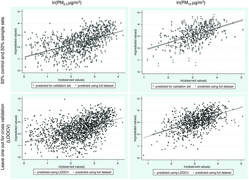
Two methods were used to validate the predicted PM. In the first method, we utilized leave one out for cross-validation (LOOCV). In this method, one data point was skipped iteratively and its value was predicted using the rest of data points. In the second method, we partitioned data points into two sets—a sample set (used for developing the model) and a control set. The sample set was used to run the model and predict values for the control set. The results are presented in Table 8 and Figure 6. The overall root mean square error (RMSE) was 2.74 and 2.67 μg/m³ for PM_2.5 by using LOOCV and a validation set. Further, the validation analysis suggests that the average values of PM_2.5 and PM₁₀ predicted using all data points and that predicted for the validation set are not significantly different (Table 8). The site-specific model outperforms the global model; for example, the average observed concentration of PM_2.5 at site number 60 was 12.792 μg/m³, but the value predicted using the global model in LOOCV was 21.162 μg/m³. However, the value predicted using the site-specific model (for the validation set LOOCV) was 12.92 μg/m³, very close to the observed value.

FIG. 6 PM₁₀ and PM_2.5 predictive model and validation. (Figure available in color online.)

3.5. Time and Space Resolved Estimates of PM

Utilizing the PM predictive model [as in Equation (4)], PM_2.5, PM₁₀, and PM_10–2.5 were predicted for all valid AOD_MODIS data points from 2000 to 2009. This resulted in a total of 2.34 million valid data points (Table 9). On average, more than 120,000 PM values were available for each year for each satellite within the geographic extent of the Cleveland MSA (82.4°W to −81°W and 40.8°N to 41.9°N); since 2003, the number of data points doubled within the same geographic extent after the launch of the Aqua satellite in May 2002, and the hourly extent of these data became 9 a.m. to 3 p.m. local time. As evident from Table 9, the average concentrations of PM from Terra were significantly higher than that from Aqua. These differences in PM estimates from Terra and Aqua can be attributed to the change in the concentration of traffic during peak and off-peak hours; the local overpass time of Terra corresponds with the peak traffic hours, and Aqua overpass time corresponds with the off-peak hours. Thus, PM estimates from Terra (peak hours) and Aqua (off-peak hours) combined can provide the robust estimates of daily PM concentration on a given day.

TABLE 9 Yearly averages of predicted PM ± 95 CI (μg/m³) and number of data points for which the predicted PM values are available in parentheses

	Terra (local crossing time 10:30 a.m.)			Aqua (local crossing time 1:30)			Terra and aqua combined
Year	PM2.5	PM10	PM10–2.5	PM2.5	PM10	PM10–2.5	PM2.5	PM10	PM10–2.5
2000	12.1 ± 0.07 (122,438)	17.5 ± 0.10 (122,438)	5.4 ± 0.03 (122,438)	Data not available (because aqua was launched in May 2002)			12.1 ± 0.07 (122,438)	17.5 ± 0.10 (122,438)	5.4 ± 0.03 (122,438)
2001	11.7 ± 0.05 (159,868)	17.0 ± 0.07 (159,868)	5.3 ± 0.02 (159,868)				11.7 ± 0.05 (159,868)	17.0 ± 0.07 (159,868)	5.3 ± 0.02 (159,868)
2002	15.2 ± 0.07 (161,733)	20.6 ± 0.09 (161,733)	5.4 ± 0.02 (161,733)	14.3 ± 0.11 (64,809)	18.8 ± 0.14 (64,809)	4.5 ± 0.03 (64,809)	14.9 ± 0.06 (226,542)	20.1 ± 0.07 (226,542)	5.2 ± 0.02 (226,542)
2003	13.5 ± 0.06 (156,044)	18.9 ± 0.08 (156,044)	5.4 ± 0.02 (156,044)	11.9 ± 0.07 (118,938)	16.4 ± 0.09 (118,938)	4.5 ± 0.02 (118,938)	12.8 ± 0.05 (274,982)	17.8 ± 0.06 (274,982)	5.0 ± 0.02 (274,982)
2004	12.6 ± 0.06 (120,351)	17.6 ± 0.09 (120,351)	5.1 ± 0.02 (120,351)	9.5 ± 0.06 (102,889)	13.7 ± 0.08 (102,889)	4.2 ± 0.02 (102,889)	11.2 ± 0.04 (223,240)	15.8 ± 0.06 (223,240)	4.6 ± 0.02 (223,240)
2005	13.2 ± 0.07 (148,310)	18.6 ± 0.10 (148,310)	5.4 ± 0.03 (148,310)	11.9 ± 0.07 (116,863)	16.6 ± 0.09 (116,863)	4.7 ± 0.03 (116,863)	12.6 ± 0.05 (265,173)	17.7 ± 0.07 (265,173)	5.1 ± 0.02 (265,173)
2006	10.9 ± 0.07 (139,498)	15.7 ± 0.09 (139,498)	4.8 ± 0.03 (139,498)	9.4 ± 0.06 (131,098)	13.7 ± 0.08 (131,098)	4.3 ± 0.02 (131,098)	10.1 ± 0.04 (270,596)	14.7 ± 0.06 (270,596)	4.6 ± 0.02 (270,596)
2007	13.1 ± 0.06 (157,787)	18.0 ± 0.08 (157,787)	4.8 ± 0.02 (157,787)	12.0 ± 0.06 (136,258)	16.5 ± 0.08 (136,258)	4.6 ± 0.02 (136,258)	12.6 ± 0.04 (294,045)	17.3 ± 0.06 (294,045)	4.7 ± 0.02 (294,045)
2008	10.6 ± 0.05 (145,621)	14.7 ± 0.07 (145,621)	4.2 ± 0.02 (145,621)	10.3 ± 0.05 (119,616)	14.5 ± 0.07 (119,616)	4.2 ± 0.02 (119,616)	10.5 ± 0.04 (265,237)	14.6 ± 0.05 (265,237)	4.2 ± 0.02 (265,237)
2009	8.8 ± 0.05 (131,884)	12.9 ± 0.07 (131,884)	4.2 ± 0.02 (131,884)	8.0 ± 0.04 (120,472)	11.9 ± 0.06 (120,472)	3.9 ± 0.02 (120,472)	8.4 ± 0.03 (252,356)	12.4 ± 0.05 (252,356)	4.1 ± 0.01 (252,356)
Total	12.2 ± 0.02 (1,443,534)	17.2 ± 0.03 (1,443,534)	5.0 ± 0.01 (1,443,534)	10.7 ± 0.02 (910,943)	15.1 ± 0.03 (910,943)	4.4 ± 0.01 (910,943)	11.7 ± 0.01 (2,354,477)	16.4 ± 0.02 (2,354,477)	4.8 ± 0.01 (2,354,477)

The predicted PM values can be used to impute daily (at any other coarser temporal scale) estimates of PM_2.5, PM₁₀, and PM_10–2.5 at any spatial resolution within the extent of the study area. As an example, PM_2.5 and PM₁₀ surfaces were generated for four different days (December 1, 4, 6, and 12, 2009) in the first 2 weeks of December 2009. Although valid PM data were also available on other days, more than 2200 data points were available on the selected 4 days (Figures 7a and b) within the geographic extent of the study area. As evident from these figures, there were subtle differences in the spatial and temporal (daily) variations in the distribution of PM_2.5 and PM₁₀, but the relative trends of PM₁₀ and PM_2.5 remained the same across these 4 days. Since emission sources remain static, it is likely to dictate the spatial trend of PM concentration with respect to these sources. However, atmospheric processes that transport aerosols (along with the PM mass) can influence the overall concentration of PM. Therefore, it is important to account for the spatial and temporal variability in predicting PM.

4. DISCUSSION

Several important findings emerge from this research. First, the 2-km AOD_MODIS, aggregated within short spatiotemporal intervals, correlates better with the in situ measurements of AOD_AERONET, because the degree of uncertainty in AOD_MODIS tends to increase as the spatial resolution of AOD_MODIS retrieval becomes coarser and the spatiotemporal intervals used for aggregating these data increase. A strong and positive correlation (>0.8) of AOD_MODIS (at all three spatial resolutions) with the AOD_AERONET also indicates the presence of a very strong spatiotemporal autocorrelation in AOD_MODIS. An improvement in the correlation coefficient from 0.85 to 0.92 for the 2-km AOD_MODIS within 0.025° and 15-min intervals suggests that the 2-km AOD_MODIS is likely to capture local spatial variability in AOD_MODIS, contributed by local emission sources. Second, PM concentration records a significant spatial variability within the study area. These data, monitored at sparsely distributed EPA sites, are not adequate to develop a systematic grid of time and space resolved estimates of ambient PM. But these data can be utilized to develop an empirical model for predicting PM wherever AOD_MODIS and other subsidiary data are available. Third, the PM prediction using AOD_MODIS can be influenced by meteorological conditions, because of a strong influence of meteorological conditions on the spatiotemporal dynamics of AOD_MODIS. Our analysis suggests that instrumenting AOD_MODIS on meteorological conditions can pave the way to develop an effective PM predictive model. Fourth, the difference between the observed and predicted values of PM was significantly greater in the downtown urban areas as compared with that in the suburban areas; likewise, the performance of the regression model was significantly better in the suburban areas than in the downtown areas.

At the 2-km spatial resolution, 2.3 million AOD_MODIS and their corresponding predicted PM values were available within the geographic extent of the study area between 2000 and 2009. This suggests that the fine resolution AOD_MODIS, computed using the data from MODIS (onboard Terra and Aqua satellites with peak and off-peak hours of overpass times, respectively), holds a great potential to characterize and quantify short- and long-term spatiotemoporal variability in PM and to develop daily estimates of PM at any spatial resolution.

Although this article empirically documents the application of the 2-km AOD_MODIS (coupled with meteorological conditions and seasonal and temporal structure) for developing time and space resolved estimates of PM, a number of limitations remain. First, the performance of the PM predictive model varies across geographic space; the model worked better for suburban than for downtown areas. For example, the difference between the predicted and observed values was significantly smaller in the suburban areas as compared with that in the downtown areas. These differences can arise due to either uncertainty in AOD_MODIS retrieval over bright surfaces and complex urban structures, or significantly greater spatial heterogeneity (due to poor dispersion and mixing of PM caused by the presence of high-rising buildings) in the PM distribution in the downtown areas. This also means that PM monitored at point locations in the downtown areas may not truly represent PM concentration in its surrounding areas.

Second, the proposed model overpredicts the low PM_2.5 concentrations (<2 μg/m³) and underpredicts the high concentrations of PM₁₀ (>120 μg/m³). The performance of site-specific models was significantly better than that of the global model. Despite this, it is important to develop region-specific models, because many regions do not have sufficient monitoring stations to develop site-specific models. Nonetheless, further research investigation is needed to understand the sources of these overpredictions and underpredictions in the PM predictive model.

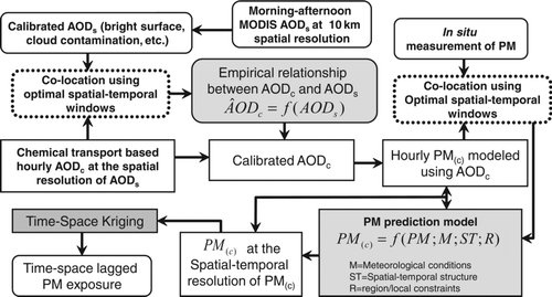
Third, AOD_MODIS retrievals can be biased in the presence of snow on the ground, bright surfaces, and cloud contamination despite the fact that the algorithm used for retrieving AOD_MODIS filters for snow cover and cloud contamination. NASA is also developing a newer version (called deep blue) to overcome uncertainty in the AOD_MODIS retrieval caused by bright surfaces. The integration of AOD_MODIS with the chemical transport model (CTM) may also help overcome many of these known problems of AOD_MODIS. CTM can be used to compute the missing AOD_MODIS values due to cloud cover, snow cover, surface brightness, and poor quality flag. The future research should be geared toward assimilation of the best strengths of these two methodologies and develop an association between AOD from CTM (AOD_CTM) and AOD_MODIS (Kumar 2010a). A conceptual framework for such an approach is presented in Figure 8. The AOD_CTM can be estimated at any temporal scale/resolution (but at a coarser spatial resolution), and its quality is largely guided by the quality of emission inventory data. An empirical relationship can be developed between AOD_MODIS and AOD_CTM, and based on this relationship, AOD_MODIS can be predicted for the missing AOD_MODIS data.

FIG. 7 (a) Daily predicted PM_2.5 surface on several days in December 2009 in the Cleveland MSA. (b) Daily predicted PM₁₀ surface on several days in December 2009 in the Cleveland MSA. (Figure available in color online.)

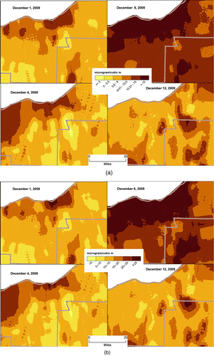
FIG. 8 A conceptual framework for the assimilation of satellite-based AOD and AOD from CTM (AOD_C) to develop time-space resolved estimates of PM.

The PM predictive model, described earlier, predicts PM at the spatiotemporal scales of AOD_MODIS data. However, for epidemiological studies, it is important that these data are available at the spatiotemporal scales of health data. In this research, we employed spatiotemporal Kriging to develop a systematic grid of daily PM at the 5-km spatial resolution. The spatiotemporal Kriging minimizes interpolation error (De Cesare et al. 2001; Dryden et al. 2005) and can be utilized to interpolate PM at any spatiotemporal scales.

Despite the limitations identified here, the 2-km AOD_MODIS is critically important for air quality studies, because local variation in AOD that results from local emission sources can be captured by the 2-km AOD_MODIS. However, this variability is generalized and does not show up in the 10-km AOD_MODIS. In addition, the number of data points in the 2-km AOD_MODIS dataset is 20–25 times higher than that in the 10-km AOD_MODIS dataset.

Acknowledgments

The United States Environmental Protection Agency through its Office of Research and Development partially funded and collaborated in the research described here under RFQ-RT-10–00204 to the University of Iowa. It has been subjected to Agency Review and approved for publication. This research was supported by NIH (R21 ES014004–01A2) and EPA (R833865; RFQ-RT-10–00204). We would like to thank the two anonymous referees for providing us with constructive comments and suggestions that allowed us to improve the quality of the initial submission.

Notes

***p < 0.01.

**p < 0.05.

***p < 0.01.

**p < 0.05.

*p < 0.1.

REFERENCES

- Boddy , J. W. D. , Smalley , R. J. , Dixon , N. S. , Tate , J. E. and Tomlin , A. S. 2005 . The Spatial Variability in Concentrations of a Traffic-Related Pollutant in Two Street Canyons in York, UK—Part I: The Influence of Background Winds . Atmos. Environ. , 39 : 3147 – 3161 .
- Chu , A. , ed. 2006 . Analysis of the Relationship Between MODIS Aerosol Optical Depth and PM2.5 in the Summertime US , San Diego, CA : SPIE Digital Library .
- Chu , D. A. , Kaufman , Y. J. , Ichoku , C. , Remer , L. A. , Tanre , D. and Holben , B. N. 2002 . Validation of MODIS Aerosol Optical Depth Retrieval over Land. Geophys . Res. Lett. , 29 ( 12 ) : 1617
- Chu , D. A. , Kaufman , Y. J. , Zibordi , G. , Chern , J.-D. , Mao , J.-M. , Li , C. and Holben , H. B. 2003 . Global Monitoring of Air Pollution over Land from EOS-Terra MODIS . J. Geophys. Res. , 108 : 4661
- De Cesare , L. , Myers , D. E. and Posa , D. 2001 . Product-Sum Covariance for Space-Time Modeling: An Environmental Application . Environmetrics , 12 : 11 – 23 .
- De Iaco , S. , Myers , D. E. and Posa , D. 2002 . Space-Time Variograms and a Functional Form for Total Air Pollution Measurements . Comput. Stat. Data Anal. , 41 : 311 – 328 .
- Dryden , I. L. , Markus , L. , Taylor , C. C. and Kovacs , J. 2005 . Non-Stationary Spatiotemporal Analysis of Karst Water Levels . J. Roy. Stat. Soc. C-Appl. Stat. , 54 : 673 – 690 .
- Dubovik , O. , Smirnov , A. , Holben , B. N. , King , M. D. , Kaufman , Y. J. , Eck , T. F. and Slutsker , I. 2000 . Accuracy Assessments of Aerosol Optical Properties Retrieved from Aerosol Robotic Network (AERONET) Sun and Sky Radiance Measurements . J. Geophys. Res.-Atmos. , 105 : 9791 – 9806 .
- Environmental Protection Agency . 2008 . Envirofacts Data Warehouse Retrieved from http://www.epa.gov/enviro/
- Gupta , P. and Christopher , S. A. 2009a . Particulate Matter Air Quality Assessment Using Integrated Surface, Satellite, and Meteorological Products: 2. A Neural Network Approach . J. Geophys. Res.-Atmos. , : 114 ISI:000271318200002D14205
- Gupta , P. and Christopher , S. A. 2009b . Particulate Matter Air Quality Assessment Using Integrated Surface, Satellite, and Meteorological Products: Multiple Regression Approach . J. Geophys. Res.-Atmos. , : 114 D20205ISI:000268631700001
- Gupta , P. , Christopher , S. A. , Wang , J. , Gehrig , R. , Lee , Y. and Kumar , N. 2006 . Satellite Remote Sensing of Particulate Matter and Air Quality Assessment over Global Cities . Atmos. Environ. , 40 : 5880 – 5892 .
- Hoff , R. M. and Christopher , S. A. 2009 . Remote Sensing of Particulate Pollution from Space: Have We Reached the Promised Land? . J. Air Waste Manag. Assoc. , 59 : 645 – 675 .
- Ichoku , C. , Chu , D. A. , Mattoo , S. , Kaufman , Y. J. , Remer , L. A. , Tanre , D. , Slutsker , I. and Holben , B. N. 2002 . A Spatio-Temporal Approach for Global Validation and Analysis of MODIS Aerosol Products . Geophys. Res. Lett. , 29 ( 12 ) : 1617
- Kumar , N. 2010a . A Hybrid Approach for Predicting PM2.5 Exposure . Environ. Health Perspect. , : 118
- Kumar , N. 2010b . What Can Affect AOD–PM2.5 Association? . Environ. Health Perspect. , 118 : A2 – A3 . 10.1289/ehp.0901732
- Kumar , N. , Chu , A. and Foster , A. 2007 . An Empirical Relationship Between PM2.5 and Aerosol Optical Depth in Delhi Metropolitan . Atmos. Environ. , 41 : 4492 – 4503 .
- Kumar , N. , Chu , A. and Foster , A. 2008 . Remote Sensing of Ambient Particles in Delhi and Its Environs: Estimation and Validation . Int. J. Rem. Sens. , 29 : 3383 – 3405 .
- Levy , R. C. , Remer , L. A. , Mattoo , S. , Vermote , E. F. and Kaufman , Y. J. 2007 . Second-Generation Operational Algorithm: Retrieval of Aerosol Properties over Land from Inversion of Moderate Resolution Imaging Spectroradiometer Spectral Reflectance . J. Geophys. Res.-Atmos. , 112 ISI:000248030400002
- Li , C. , Lau , A. K.-H. , Mao , J. T. and Chu , D. A. 2005 . Retrieval, Validation and Application of 1-km Resolution Aerosol Optical Depth from MODIS Data over Hong Kong . Trans. Geosci. Rem. Sens. , 43 : 2650 – 2658 .
- Liu , Y. , Paciorek , C. J. and Koutrakis , P. 2009 . Estimating Regional Spatial and Temporal Variability of PM2.5 Concentrations Using Satellite Data, Meteorology, and Land Use Information . Environ. Health Perspect. , 117 : 886 – 892 .
- Martin , R. V. 2008 . Satellite Remote Sensing of Surface Air Quality . Atmos. Environ. , 42 : 7823 – 7843 .
- NASA . 2007 . The AERONET (AErosol RObotic NETwork), National Aeronautics and Space Administration Retrieved from http://aeronet.gsfc.nasa.gov/
- NASA . 2010 . The Level 1 and Atmosphere Archive and Distribution System, National Aeronautics and Space Administration Retrieved from http://ladsweb.nascom.nasa.gov/
- NCDC . 2007 . National Climatic Data Center, National Oceanic & Atmospheric Administration and US Department of Commerce Retrieved from http://www.ncdc.noaa.gov/oa/ncdc.html
- Ramachandran , S. 2007 . Aerosol Optical Depth and Fine Mode Fraction Variations Deduced from Moderate Resolution Imaging Spectroradiometer (MODIS) over Four Urban Areas in India . J. Geophys. Res.-Atmos. , : 112 Artn D16207:10.1029/2007jd008500
- Remer , L. A. , Kaufman , Y. J. , Tanre , D. , Mattoo , S. , Chu , D. A. , Martins , J. V. , Li , R. R. , Ichoku , C. , Levy , R. C. , Kleidman , R. G. , Eck , T. F. , Vermote , E. and Holben , B. N. 2005 . The MODIS Aerosol Algorithm, Products, and Validation . J. Atmos. Sci. , 62 : 947 – 973 .
- Remer , L. A. , Tanré , D. and Kaufman , Y. J. 2006 . Algorithm for Remote Sensing of Tropospheric Aerosol from MODIS, NASA , Greenbelt, MD : Goddard Space Flight Center97 NASA . Retrieved from http://modis.gsfc.nasa.gov/data/atbd/atbd_mod02.pdf
- Smirnov , A. , Holben , B. N. , Eck , T. F. , Dubovik , O. and Slutsker , I. 2000 . Cloud-Screening and Quality Control Algorithms for the AERONET Database . Remote Sens. Environ. , 73 : 337 – 349 .
- 2010 . “ StataCorp ” . In STATE/SE Version 10.1 , College Station, TX : StataCorp LP . USA
- Tripathi , S. N. , Srivastava , A. B. K. , Dey , S. , Satheesh , S. K. and Krishnamoorthy , K. 2007 . The Vertical Profile of Atmospheric Heating Rate of Black Carbon Aerosols at Kanpur in Northern India . Atmos. Environ. , 41 : 6909 – 6915 .
- van Donkelaar , A. , Martin , R. V. , Brauer , M. , Kahn , R. , Levy , R. , Verduzco , C. and Villeneuve , P. J. 2010 . Global Estimates of Ambient Fine Particulate Matter Concentrations from Satellite-Based Aerosol Optical Depth: Development and Application . Environ. Health Perspect. , 118 : 847 – 855 .
- Wang , J. and Christopher , S. A. 2003 . Intercomparison Between Satellite-Derived Aerosol Optical Thickness and PM2.5 Mass: Implications for Air Quality Studies . Geophys. Res. Lett. , 30 : 2095
- Zhang , J. L. and Reid , J. S. 2006 . MODIS Aerosol Product Analysis for Data Assimilation: Assessment of Over-Ocean Level 2 Aerosol Optical Thickness Retrievals . J. Geophys. Res.-Atmos. , : 111 Artn D22207: Doi 10.1029/2005jd006898