Inertial Particle Deposition in a 90° Laminar Flow Bend: An Eulerian Fluid Particle Approach

Abstract

A numerical model for the simulation of aerosol flows via an Eulerian–Eulerian, one-way coupled, two-phase flow description is presented. An in-house computational fluid dynamics code is used to simulate the gaseous (continuous) phase, whereas a modified convective diffusion equation models particle transport. The convective diffusion equation, which includes inertial, gravitational, and diffusive particle transport, is solved by computational fluid dynamics techniques. The model is validated by comparing the calculated laminar fluid flow and particle deposition fractions to analytical and experimentally studied aerosol flows in a laminar flow 90° bend of circular cross section available in the literature. Model predictions are also compared with numerical predictions of Eulerian-Lagrangian models. Particle concentration profiles at different cross sections are calculated, and deposition sites on the wall boundary are indicated. For the range of studied particle diameters, the Eulerian–Eulerian model predicts deposition fractions satisfactorily, being in good agreement with the experimental data.

LIST OF SYMBOLS

Latin	=
c	=	particle concentration
Cc	=	Cunningham slip correction factor
	=	gravitational settling velocity vector
De	=	Dean number
dp	=	particle diameter
dt	=	tube diameter
Fr	=	Froude number
	=	gravity vector
Jc	=	convective flux
Jd	=	diffusive flux
	=	Cartesian basis vectors
k	=	gravitational settling parameter
L	=	tube length
	=	normal to the surface unit vector
p	=	fluid pressure
Pe	=	Peclet number
Peth	=	thermal Peclet number
Rb	=	bend radius
Re	=	Reynolds number
Ro	=	bend curvature ratio
rt	=	tube radius
	=	surface area vector
St	=	Stokes number
T	=	temperature
T	=	time
	=	fluid velocity vector
u, ν, w	=	Cartesian components of fluid velocity
	=	particle velocity vector
Greek	=
ϵ	=	relative error
ϵ RMS	=	root-mean-square of the relative error
η	=	deposition fraction
μ f	=	fluid dynamic viscosity
ρ f	=	fluid density
ρ p	=	particle density
τ ij	=	components of the stress tensor
τ p	=	particle relaxation time
dΩ	=	elemental volume
Subscripts	=
f	=	fluid
m	=	mean
p	=	particle
T	=	tube
w	=	wall

ABBREVIATIONS

CDS	=	central differences discretization
CFD	=	computational fluid dynamics
CVs	=	computational volumes
PBE	=	population balance equation
UDS	=	upwind discretization scheme

INTRODUCTION

Particle deposition in bends is an important removal mechanism in many industrial and biological aerosol processes. Sampling and transport of particles in high-purity gas streams, synthesis and processing of materials using aerosol routes, as well as flow characterization techniques based on aerosol diagnostics are few examples of industrial processes in which particle losses may affect the desired output. The deposition of inhaled particles on human airways, inhaled either from ambient air or as medicinal drugs, is a process important for biological and health effects. In all these processes, particle transport in bends, and specifically particle deposition, plays a significant role.

The most extensive experimental study of particle deposition in a 90° bend of circular cross section up to now has been conducted by Pui et al. (1987). Measurements were performed for both laminar and turbulent flows using monodisperse aerosol populations. The bends were of different tube diameters d_t (or radii r_t ) and the bend curvature ratios R_o , defined as R_o =R_b /r_t with R_b the bend radius, varied from 5.6 to 7.

Numerical investigations of particle deposition due to the fluid-inertia-induced secondary flow have also been carried out. The Lagrangian description of the particulate phase, whereby the particle equations of motion are solved to determine the deposition efficiency [either numerically Breuer et al. (2006), Crane and Evans (1977), Tsai and Pui (1990), or analytically Cheng and Wang (1975, 1981)], is the most frequent choice because it provides a convenient and easy method to treat inertial effects. However, the determination of some average quantities, for example, the local particle concentration field (Slater and Young 2001) or the mean interphase momentum transfer (Garg et al. 2009), can be particularly difficult. A large number of particle trajectories have to be calculated to minimize statistical error (Desjardins et al. 2008), rendering the Lagrangian approach computationally inefficient. The control of the numerical error associated with Lagrangian-Eulerian simulations becomes more important for highly nonuniform spatial distributions of particles as the number of simulated particles in a grid cell decreases; accordingly, the statistical error, which is inversely proportional to the square root of the number of particles per cell, increases. Recent advances in numerical implementations of Lagrangian-Eulerian method have addressed this issue by introducing improved error estimators to obtain numerically convergent simulations (Garg et al. 2009).

A distinct advantage of the Lagrangian approach is that it easily captures particle trajectory crossings for finite inertia (finite Stokes number) particles, namely, cases in which the particle velocity distribution is not unimodal and a finite probability exists that particles at the same location have different velocities. Such situations may occur when two particle jets cross, when a particle jet impinges on a surface and it rebounds, or for finite Stokes number particle flows in Taylor–Green vortices. A recently proposed quadrature-based Eulerian moment closure was shown to predict accurately flows with particle-crossing trajectories (Desjardins et al. 2008).

Notable alternatives to the Eulerian-Lagrangian calculations are the works of Armand et al. (1998) and Lawson et al. (2006). The latter attempted to calculate the particle concentration in a bend by a full Lagrangian method (Healy and Young 2005). Accordingly, the particle concentration was determined by calculating the deformation (dilation or compression) of an infinitesimal rectangular volume along the trajectory of a single particle. The former proposed and validated, in both laminar and turbulent regimes, a Eulerian approach that included inertial particle drift in a two-fluid model. The particle velocity was determined by solving numerically the coupled dispersed-phase mass and momentum equations.

The particle population balance equation (PBE) in a Eulerian description examines aerosol processes (e.g., transport, nucleation, growth, and coagulation) in a fixed elemental volume: diffusion, thus, is treated directly and particle concentration is calculated in a straightforward manner. However, inertial effects cannot be easily included in the standard form of PBE. Here, an approximate expression for the particle velocity is used to incorporate inertial effects in a Eulerian formalism.

This Eulerian approach offers significant advantages over two fluid models that do not decouple the mass and momentum conservation equations of the dispersed phase. First, the numerical solution of the particle momentum equation is not required to determine the particle velocity field, as the momentum equation has been solved perturbatively. As a result, the particle velocity is expressed solely in terms of the fluid velocity and its spatial derivatives (in steady state). Moreover, it can be used for small particle diameters where the particle equations of motion in a Lagrangian approach become numerically stiff. Finally, it is more accurate than passive tracer models as it can take into account simultaneous diffusive and inertial particle transport.

Efforts along this direction have already been made for submicrometer particles. Longest and Oldham (2008) developed an Eulerian–Eulerian model to predict particle deposition in a laminar-bifurcating flow system for cases in which diffusion and inertia are important for particle deposition. They extended the drift flux approach with near-wall corrections to account for particle deceleration between the nearest control volume center and the wall surface. Xi and Longest (2008a) extended this Eulerian–Eulerian model to also account for aerosol dispersion in both turbulent and unsteady flows, and they applied the model to predict deposition in a realistic model of the tracheobronchial airways. Moreover, Xi and Longest (2008b) applied the Eulerian–Eulerian model to predict particle deposition due to inertia, diffusion, and turbulent dispersion in a complex model of the nasal cavity. Similarly, Zhao et al. (2009) presented a generalized drift-flux model for turbulent flows of ultrafine particles in indoor environments. These studies also reported particle concentration and deposition profiles.

In this work, we use a similar Eulerian–Eulerian description of a dilute dispersed flow in the limit of low mass loading and low volume fractions. One-way coupling of the dispersed phase is considered, whereby the dispersed-phase motion is affected by the continuous phase, but not vice versa. In the Eulerian description of the dispersed phase, we approximate the particle velocity in the mass conservation equation of the dispersed (particulate) phase, or equivalently the PBE, by an expression obtained in the limit of low particle relaxation time. The particle velocity is decomposed into a diffusive term, which depends on the particle concentration gradient, and a convective term, independent of particle concentration. The convective particle velocity becomes the fluid velocity corrected by the inertial drift (or slip) and the gravitational settling velocities, thereby introducing particle inertial and gravitational effects in the Eulerian form of the PBE. The main goal of the present work is to study the validity of the particle velocity approximation for higher particle relaxation times. In order to do so, the simple bend geometry and laminar flow field were chosen and we focused on coarse particles (5 μm⩽d_p ⩽20 μm), where inertial effects are important and gravity may not be neglected a priori.

The modified PBE is solved numerically in three dimensions using computational fluid dynamics (CFD) techniques. Particle concentration is obtained by imposing the commonly used condition of totally absorbing wall (zero particle concentration at the wall). The particle deposition flux is calculated as the sum of a convective and diffusive flux. The numerical results of the Eulerian fluid particle model are compared with benchmark solutions available in literature.

MODEL DESCRIPTION

Continuous Phase: Numerical Method

The in-house CFD code developed by Neofytou and Tsangaris (2006) is used to solve the Navier–Stokes equations for the three-dimensional incompressible flow field of the carrier fluid. The mass continuity equation in integral form is

and the momentum equations are

In the above equations, is the fluid velocity, p is the pressure, ρ _f is the fluid density, τ _ij is the components of the stress tensor, is the elemental surface with as the normal to the surface unit vector, dΩ is the elemental volume, and are the Cartesian basis vectors.

The code uses the SIMPLE scheme incorporated in a finite volume method with a collocated arrangement of variables, and it enables multiblock computations. The discretization of the convection terms is performed using the QUICK difference scheme of the third order. A solution is reached assuming Newtonian fluid, laminar flow, constant fluid properties, and one-way coupling, i.e., the influence of the particulate phase on the hydrodynamic field of the carrier fluid is considered negligible. A parabolic velocity profile at the inlet was chosen, and a no-slip fluid velocity condition was imposed at the wall boundaries.

Dispersed Phase: Governing Equations

The general form of the PBE for a monodisperse particle population in a flowing fluid is

where c is the particle concentration and is the particle velocity. The first term on the left-hand side refers to particle accumulation and the second refers to particle transport, whereas the first term on the right-hand side represents gas-to-particle conversion processes and the second represents coagulation or agglomeration. Equation (3) is the mass conservation equation of the particulate phase.

Here, we focus on the transport of a population of particles, i.e., the PBE is examined neglecting the internal processes of the right-hand side of Equation (3). The mass conservation equation under steady-state conditions becomes

The effect of inertia on Brownian diffusive transport in isothermal aerosol flows under steady-state conditions was considered by Fernandez de la Mora and Rosner (1982). Stokes’ drag was assumed (particle Reynolds number much smaller than unity) and the particle density was taken to be much higher than the carrier-flow density. They solved the particle momentum equation for the particle velocity to the first order in the particle relaxation time τ _p (the inverse of Stokes friction coefficient per unit mass):

where μ _f is the fluid dynamic viscosity, ρ _p and d_p are the particle density and diameter, C_c is the Cunningham slip correction factor, and χ is the particle dynamic shape factor. The last two factors are unity for spherical particles of diameters greater than 1 μm, such as those considered in this study. They obtained the first-order correction to the particle velocity due to particle inertia:

where D is the particle Stokes-Einstein diffusion coefficient, D=k_BT/3πμ _f d_p , with k_B as Boltzmann constant and T is the fluid temperature. If we also take into consideration gravity, Equation (6) becomes

where is the velocity due to gravitational settling:

with as the gravity vector (Drossinos and Housiadas 2006). For the aerosol under study, ρ _f <<ρ _p , thus Equation (8) is written as

The particle velocity is, thus, decomposed into two parts: a diffusive part, dependent only on the particle concentration gradient, and a convective part , independent of particle concentration. In particular, the convective particle velocity

depends only on the fluid velocity and its spatial gradients and it incorporates the effects of particle inertia and gravity.

The low-τ _p expansion of the particle velocity decouples the mass and momentum conservation equations for the dispersed phase. Therefore, the dispersed-phase mass conservation, Equation (4), takes the form of a modified steady-state convective diffusion equation:

Equation (11) incorporates the effects of particle convection, inertia, and diffusion in an Eulerian formalism to the first order in the particle relaxation time. In the dimensionless and integral form, it becomes (to simplify notation, we retain the same variables to denote dimensionless quantities)

where St=τ _p υ _o /r_t is the particle Stokes number, with υ _o as the mean axial fluid velocity (to be taken the mean fluid velocity at the tube inlet), Fr=υ² _o /gr_t is the Froude number, and Pe=d_t υ _o /D is the mass Peclet number, a function of the particle diameter through D. Length scales are scaled by the tube diameter d_t and velocities by υ _o . Equation (12) expressed in terms of the (dimensionless) particle convective velocity becomes

The modified convective diffusion equation written in the form of Equation (13) resembles the usual convective diffusion equation and, thus, it can be numerically treated similarly.

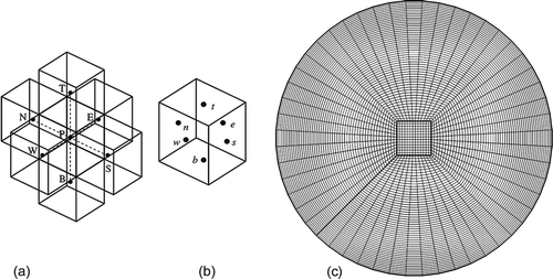
FIG. 1 (a) Grid topology, (b) control volume, and (c) grid cross section.

Dispersed Phase: Boundary Conditions

At the inlet, a plug concentration particle profile was used (inlet concentration of unity in the dimensionless form). The particle concentration wall boundary condition was the usual condition of a totally absorbing wall:

which at the wall boundary gives a (dimensionless) diffusive flux,.J^d | _w , equal to

Moreover, there is a finite nonzero particle convective velocity just before the wall, due to the external forces [Equation (10)], resulting in a (dimensionless) convective flux, J^c | _w , which can be written as

where the particle convective velocity, , is calculated just before the wall boundary, i.e., at the computational grid point closest to the wall. Hence, if the convective flux at the grid point closest to the wall is toward the wall, the depositing convective flux at the wall is equal to it; otherwise, the convective flux at the wall is zero. The two cases of Equation (16) are necessary to take the convective flux into account only when it indicates that particles would exit the wall boundaries. The influx of particles from the wall is not permitted, because it is physically unrealistic in the present study. Therefore, the total (dimensionless) deposition flux becomes

Longest and collaborators (Longest and Oldham 2008; Xi and Longest 2008a, 2008b) used Equation (17) to calculate the deposition fraction of inertial particles as the sum of a convective and a diffusive term. Furthermore, they analyzed two other alternatives to specify the convective flux at the wall. They found that a velocity correction based on a subgrid Lagrangian solution improved numerical predictions for the local and regional deposition fractions of fine respiratory aerosols. We do not expect that this correction would modify significantly our deposition fraction results because we simulate high inertia particles (high Stokes number particles), whose velocity responds slowly to changes of the fluid velocity. Their velocity at the center of the computational grid closest to the wall persists for a longer time than that of fine aerosol particles (d_p ⩽1 μm). More importantly, in our simulations gravity, a body force independent of the fluid velocity acts on these particles.

The modified convection–diffusion equation, Equation (11) or (12), was obtained from the leading-order correction of the particle velocity in terms of the particle relaxation time (in a low Stokes number expansion). It arises from a perturbative solution of the particle-phase momentum conservation equation. Consequently, it captures the leading-order effect of particle inertia on the usual convective diffusion equation, and hence, it becomes important when both inertial and diffusive particle transport occur simultaneously [for an analysis of the low Stokes number expansion in a simple shear flow, and the decoupling of the two continuum conservation equations, see Drossinos and Reeks (2005)]. In the following section, the modified convective diffusion equation will be used to model deposition of nonzero, finite Stokes number particles in a laminar flow bend.

Furthermore, the range of validity of the low Stokes number expansion has not been specified. Ferry and Balachandar (2001) investigated the range and in particular the uniqueness of the Eulerian particle velocity field as a function of τ _p , in the absence of diffusion and with elastic particle rebound at the walls. Although they derived an inequality specifying how small τ _p should be, they ascertained the accuracy of the expansion through a comparison of the particle velocity obtained by Lagrangian particle tracking and the Eulerian method truncated at various orders (zeroth, first, and second) in a turbulent channel flow. They found that for small τ _p (specifically, when the particle response time normalized by the fluid time scale is less than unity), the first-order approximation gave a significant improvement over the zeroth-order term, but the second-order correction did not lead to further improvements. In this work, where in addition, a concentration boundary layer exists and particles diffuse, the validity of the approximation is ascertained by comparing our results with experimental data and previous simulations.

Dispersed Phase: Numerical Solution

Once the fluid velocity is numerically obtained, the convective particle velocity is calculated using Equation (10). The modified convection–diffusion equation is subsequently solved in three dimensions using a finite volume method with a collocated arrangement of variables, a numerical scheme analogous to that used for the carrier fluid flow. The convective-velocity term is treated by a deferred-correction approach to avoid a direct application of high-order schemes that would result in big computational molecules (Ferziger and Peric 2002). Thus, the convective term is discretized into an implicit part in which a first-order upwind scheme (UDS) is used, and an explicit part composed of the difference between the UDS and the second-order central difference scheme (CDS). Once the iterations converge, the lower-order scheme (UDS) cancels out and the obtained solution corresponds to the higher-order scheme (CDS). The second-order CDS is preferred for the diffusive term. The topology of the grid (Neofytou and Tsangaris 2006) and the control volume are shown in Figure 1a and b.

The discretized form of Equation (12) applied on a computational cell leads to the following algebraic equation:

where the subscript p denotes the computational cell, α _L are the coefficients of the unknown concentrations, and q is the source term containing all the known terms arising from the discretization. The application of Equation (18) on each cell results in a system of linear algebraic equations that are solved using the iterative strongly implicit procedure, an incomplete lower-upper decomposition method.

Dispersed Phase: Bend Geometry and Computational Grid

Deposition of a monodisperse aerosol population in a 90° bend of circular cross section was simulated adopting the geometry proposed by Pui et al. (1987) and Breuer et al. (2006). The main geometrical features of the bend are shown in Figure 2. Two linear sections, the first horizontal of length d_t at the bend inlet and the second vertical of length 2d_t at its exit, are introduced to ensure that the fluid flow in the bend is not disturbed by the inlet and outlet conditions. The diameter of a cross section of the tube at the symmetry plane is denoted as A-A, whereas the diameter of a cross section of the tube perpendicular to the symmetry plane is denoted as B-B. Given this geometry, the flow Reynolds number is Re=ρ _f υ _o d_t /μ _f and the flow Dean number is . Note that the bend radius R_b depends on the scale used to render lengths dimensionless, whereas the bend curvature ratio R_o (=R_b /r_t ) does not.

FIG. 2 (a) Geometry (R_b =2.85, R_o =5.7): A-A is the diameter of the cross section at the symmetry plane and B-B is the diameter perpendicular to it; (b) orientation of the bends for Re=100 (left) and Re=1000 (right) and the corresponding gravity vectors.

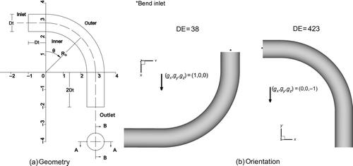
On the basis of the description of the experimental setup of Pui et al. (1987), the orientation in three-dimensional space of the tubes for Re=100 and Re=1000 are shown in Figure 2. The unit gravity vectors in each case are also noted in this figure. For the case Re=100, a vertical inlet section was used in the experimental setup to minimize particle settling in this section.

The computations were performed using a grid based on an O-type multiblock structure to avoid singularities imposed by a polar grid. The outer block is nearly polar, enclosing the square inner block as shown in Figure 1c. The grid is refined in the vicinity of the wall to capture in detail the concentration boundary layer, a region important for the calculation of particle deposition. The resolution of the grid is about 1.46×10⁶ computational volumes (CVs), consisting of about 6500 grid points in every cross section and 225 grid points in the direction of the flow.

Grid independence of the solution was tested using different grid densities. The root mean square of the relative error of the particle concentration for various grid densities is shown in Table 1. The root mean square is defined as , where ϵ _i =|(c _i,coarse −c _i,fine )/c _i,fine | is the relative error and N is the number of points used (here 300 from different regions of the computational domain). Table 1 shows that a further increase in the CVs of the chosen grid by 20% changes the concentration by less than 0.5%.

TABLE 1 A measure of grid convergence: the root mean square error of particle concentration, ε _RMS , for different coarse and fine grid densities

CVs (× 10^3)
Coarse	Fine	ε RMS (%)
276	698	4.53
698	1173	3.48
1173	1457	1.36
1457	1747	0.31

RESULTS AND DISCUSSION

Fluid Flow

FIG. 3 Axial velocity profiles at θ = 0° (inlet), θ = 45°, and θ = 90° (exit) cross sections along the diameters A-A (left) and B-B (right). (a) De=38, and (b) De=419. Results of this study are in black, and those of Tsai and Pui (1990) are in gray.

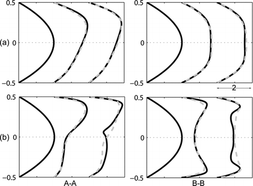
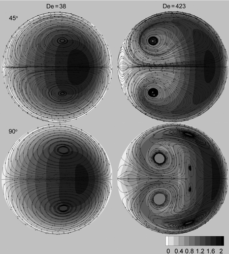
FIG. 4 Secondary flow streamlines and contours of constant axial velocity at θ=45° (top) and θ=90° (bottom) cross sections for De=38 (left) and De=423 (right).

The validity of the calculated flow field is ascertained by simulating two flows with Re=100, R_o =7 (De=38) and Re=1000, R_o =5.7 (De=419). Results are shown in Figure 3. The axial velocity profiles along the diameters A-A in the symmetry plane (left column) are skewed toward the outer bend wall due to the centrifugal forces exerted on the fluid. The axial velocity profiles along the diameters B-B, which are perpendicular to the symmetry plane (right column), are deformed but remain symmetric with respect to the symmetry plane of the bend. The deformation of the axial velocity profiles along the diameters A-A shifts toward the outer boundary wall of the bend with increasing Dean number. These results are in good agreement with the numerical solution of Tsai and Pui (1990).

The secondary flow streamlines and contours of constant axial fluid velocity are shown in Figure 4 at angles θ=45° and θ=90° along the bend for Dean numbers De=38 (left column) and De=423 (right column). The streamlines of the low Dean number secondary flow show the formation of a pair of symmetric, counter-rotating vortices, the centers of which are slightly displaced toward the outer bend wall at both angles. The main feature of the flow is the formation of an inviscid rotational core surrounded by a thin boundary layer. The peak of the axial fluid velocity is located closer to the outer wall. Our results are similar to those obtained by Pui et al. (1987) for intermediate Dean numbers (17⩽De⩽370).

The secondary flow streamlines for De=423 at 45° also show two main, symmetric counter-rotating vortices, but their centers are displaced toward the inner bend wall and they are skewed with respect to the symmetry plane. In addition, increased centrifugal forces lead to increased fluid flow toward the outer wall; the boundary layer of the secondary flow gets thinner near the outer wall and thicker near the inner wall. At θ=90°, three vortices and their symmetric with respect to the A-A diameter, are formed and the peak of the axial fluid velocity shifts further toward the outer wall. These results are in agreement with both the theoretical descriptions of Pui et al. (1987) for large Dean numbers (De⩾370) and the numerical simulations of Breuer et al. (2006).

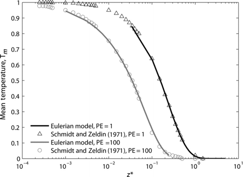
Passive Tracer (Graetz-Nusselt Problem)

The numerical discretization of the diffusive term is validated by solving the usual convective diffusion problem for a passive tracer. Given the similarities of heat and mass transfer, we simulated the Graetz-Nusselt problem (Shah and London 1978). Assuming a hydrodynamically developed fluid flow and a thermally developing temperature field, the following (dimensionless) equation was solved for a straight circular duct:

FIG. 5 Mixing temperature in a straight duct of circular cross section for different Peclet numbers.

where the thermal Peclet number is Pe_th =d_t υ₀/α, with α as the fluid thermal diffusivity. The inlet conditions are parabolic velocity profile (fully developed field), plug (constant) temperature profile at the inlet, no velocity slip at the wall, and the wall boundary condition is constant temperature. The mean (mixing) fluid temperature T_m across the duct is defined by

where is the flow area. The mean fluid temperature for different thermal Peclet numbers is shown in Figure 5; z*=z/ _th is the dimensionless axial coordinate (Shah and London 1978). The agreement of our numerical simulations with the numerical solution of Schmidt and Zeldin (1971) is excellent.

Inertial Particles: Deposition Fraction

The fraction of the deposited particles in a duct, η, is calculated by

where is the dimensionless particle flow rate through the area of bend cross section. The subscripts “inlet” and “outlet” refer to the tube inlet and outlet, respectively.

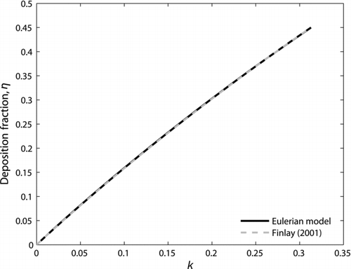
Inertial Particles: Gravitational Settling

In order to verify the gravitational term in the presented model, the problem of particle deposition in a straight horizontal tube under the sole influence of gravity is simulated. Finlay (2001) presented an analytical solution for the gravitational settling of particles in each generation of the human lung, assuming tubular geometry and Poiseuille fluid flow. For the case of the trachea (tube diameter d_t =0.018 m, length L=0.125 m, and mean inlet velocity υ _o =1.166 m/s), the results of the Eulerian model agree with the analytical solution, as shown in Figure 6. The parameter k in the figure is defined by

FIG. 6 Deposition fraction of particles sedimenting in a straight duct of circular cross section.

Inertial Particles: Bend Deposition

The inertial term in the Eulerian–Eulerian model is validated by comparing the calculated particle deposition fractions with previous theoretical calculations and experimental results. Simulations were performed for both analytical and experimental flow fields.

TABLE 2 Fluid and particle properties used in the simulations

Fluid temperature T	273 K
Fluid density ρ f	1.18 kg/m^3
Fluid dynamic viscosity μ f	1.85 × 10^−5 kg/m s
Particle density ρ p	895 kg/m^3
Particle diameter dp	5–20 μm
Dean number De=38 (Re=100,  Ro =7,  Rb =3.5)
Tube diameter dt	0.93 × 10^−3 m
Fluid mean inlet velocity υ o	1.686 m/s
Dean number De=423 (Re=1000,  Ro =5.7,  Rb =2.85)
Tube diameter dt	3.95 × 10^−3 m
Fluid mean inlet velocity υ o	3.86 m/s

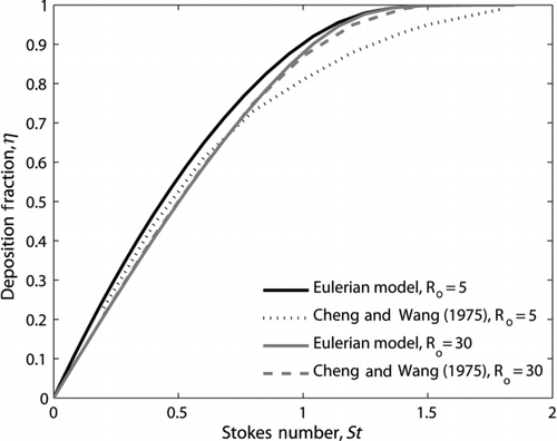
Deposition calculations without gravitational settling were performed for two bend curvature ratios (R_o =5 and 30) with the ideal flow field without secondary flow used by Cheng and Wang (1975); calculated deposition fractions are compared with their analytical results in Figure 7. The predictions of the Eulerian model agree with the analytical solution at low Stokes numbers, whereas they diverge at high Stokes numbers and at the low bend curvature ratio. The disagreement at high Stokes numbers is not unexpected because the model is based on a low Stokes number expansion. The difference is at maximum 10%, tending to zero with increasing bend curvature, i.e., as particle inertial effects become weaker.

FIG. 7 Deposition fraction—comparison with analytical results of Cheng and Wang (1975).

Simulations were also performed for experimental flows taking into account both gravitational and inertial effects and using the parameters shown in Table 2. Numerical simulations of aerosol flows for two Dean numbers (De=38  and  423) are compared to the experimental results of Pui et al. (1987), who used oleic acid aerosol particles of varying diameters from 5 to 20 μm, as well as with the Lagrangian simulations of Tsai and Pui (1990).

The Eulerian model predicts well the deposition fraction with respect to experimental data of Pui et al. (1987) for both De=38 and De=423, as shown in Figures 8 and 9 respectively.

FIG. 8 Deposition fraction for De=38—comparison with experimental measurements.

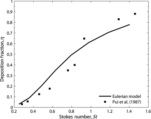
FIG. 9 Deposition fraction for De=423—comparison with experimental measurements and numerical simulations.

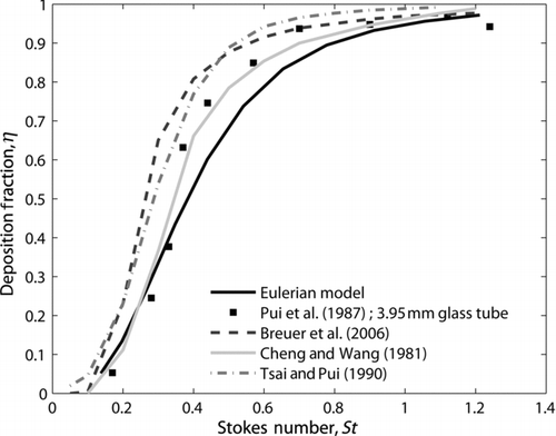
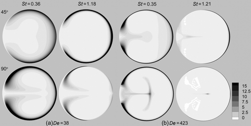
FIG. 10 Particle concentration at θ=45° (top row) and θ=90° (bottom row) cross sections along the bend. (a) De=38 (first two columns) and (b) De=423 (last two columns).

These experiments have been used repeatedly for the validation of deposition efficiency calculations via Lagrangian simulations of the particulate phase for the De=423 case. The results of some of these simulations (Cheng and Wang 1981; Breuer et al. 2006) are compared with ours in Figure 9, allowing a direct comparison of Eulerian and Lagrangian methods. The deposition fractions calculated using the Eulerian model differ from the results of Cheng and Wang (1981) (who performed Lagrangian simulations with the analytical fluid flow proposed by Mori and Nakayama [1965]) by less than 10%. However, the difference is up to 30% with the numerical results of Tsai and Pui (1990) and Breuer et al. (2006), who solved numerically for the flow field and used a different friction law. It should be noted that the aforementioned Lagrangian simulations do not take into account gravity. However, we found that gravity is not important compared to the inertial effects in this particular geometry.

Inertial Particles: Particle Concentration Profiles

One of the most appealing features of the Eulerian approach is that it allows an easy calculation of particle concentration profiles. The spatial distribution of particle concentration is presented in Figure 10 at the θ=45° and θ=90° cross sections along the bend for De=38 and St=0.36 (first column) and 1.18 (second column), and De=423 and St=0.35 (third column) and 1.21 (fourth column). The color scale was chosen to vary from 0 (light) to 15 (dark) to visualize the main features of the concentration profiles as maximum particle concentrations of approximately 570 (De=38) to 1100 (De=423) were calculated. For the low Dean number flow, lower Stokes number particles (St=0.36) follow the fluid streamlines and the main features of the secondary fluid flow can be recognized. Deposition is negligible, although there is significant particle accumulation close to the bend walls. With increasing Stokes number, and consequently inertial effects, bend deposition increases, the secondary flow persists, and particles accumulate closer to the walls. Nevertheless, particle trajectories do not deviate significantly from the gas streamlines. For the higher Stokes number (St=1.18), the particle concentration field is qualitatively different from the fluid velocity field because inertial effects dominate, almost no particles exit the bend, and the deposition fraction tends to unity. The large particle-free regions in Figure 10 make evident the difficulty to compute particle concentrations via traditional numerical implementations of Lagrangian particle tracking: a very dense particle injection grid would be required to capture the small regions, where the particle concentration is low. As mentioned in the Introduction section, for highly inhomogeneous spatial particle distributions, an improved numerical scheme, such as suggested by Garg et al. (2009), should be used in the Lagrangian simulations. These trends become more prominent for De=423 because the fluid flow is more intense.

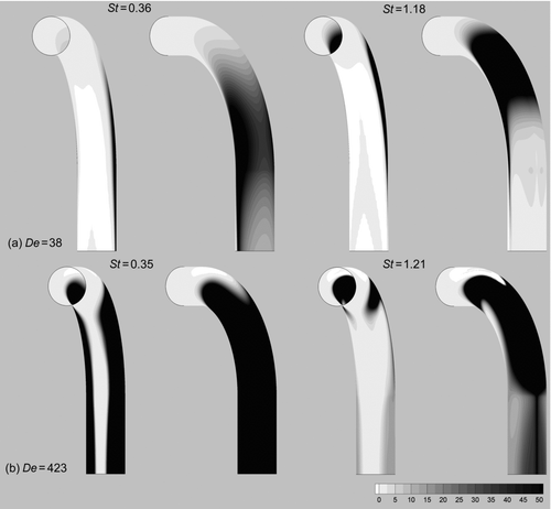
FIG. 11 Particle concentration at the wall boundary: (a) top: De=38; (b) bottom: De=423.

Inertial Particles: Deposition Sites

The location of particle deposition in terms of the particle concentration at the wall boundary is shown in Figure 11 for De=38 (top) and De=423 (bottom): the particle concentration at the computational wall boundary cell is shown. Deposition sites are shown for low and high Stokes numbers, and the bend is presented for both the inner and outer sides. For both Dean numbers and for low Stokes numbers (St=0.36 and St=0.35), significant deposition occurs toward the exit of the bend, as well as at the last straight portion of the tube. As a result of the secondary flow, a substantial amount of particles deposits on the bend side walls, in addition to those deposited on the outer wall. For high Stokes numbers (St=1.18 and St=1.21), deposition occurs closer to the bend inlet, and particles deposit mostly on the outer walls. Thus, the particle-free zone of the bend walls at the inner side is wider in this case. The aforementioned trends are particularly obvious for the higher Dean number flow. They are in agreement with both the experimental observations of Pui et al. (1987) and the calculations of Breuer et al. (2006). Moreover, a comparison of the two subfigures (a) and (b) confirms that the effect of particle inertia is considerably more intense at higher Dean numbers.

CONCLUSIONS

An Eulerian–Eulerian model was developed to simulate steady-state aerosol flows and to calculate particle deposition fractions. Particle transport due to gravity, diffusion, and inertia was incorporated in the Eulerian description of the particulate phase by adding a Stokes-number-dependent, first-order correction to the particle velocity field. Under steady-state conditions, the inertial drift correction depends only on the fluid velocity and its derivatives allowing its evaluation from the fluid velocity field without solving an additional equation, the particulate-phase momentum equation. Particle deposition was calculated from the sum of the diffusive and convective fluxes at the wall.

The Eulerian–Eulerian model was validated against analytical, numerical, and experimental results on inertia-induced particle deposition efficiencies in a 90^o laminar flow bend of circular cross section. In particular, model predictions for low Stokes numbers agreed with the analytical results of Cheng and Wang (1975), who used an ideal fluid flow without the secondary flow, slightly overestimating deposition at high Stokes numbers. Maximum difference was about 10% for the smallest bend curvature ratio, tending to zero as the curvature ratio increases, and therefore sufficiently accurate for practical purposes. Comparison of the Eulerian model with experimental data was very good for both low and high Dean number flows (De=38 and De=423). However, the model underestimated deposition with respect to numerical predictions of Eulerian-Lagrangian models. Profiles of particle concentration were calculated and sites of particle deposition along the bend were indicated.

Acknowledgments

Y. Drossinos thanks Sandy Lawson for many useful and critical discussions on the motion of particles in bends and on Lagrangian particle tracking.

REFERENCES

- Armand , P. , Bouland , D. , Pourprix , M. and Vendel , J. 1998 . Two Fluid Modeling of Aerosol Transport in Laminar and Turbulent Flows . J. Aerosol Sci. , 29 : 961 – 983 .
- Breuer , M. , Baytekin , H. T. and Matida , E. A. 2006 . Prediction of Aerosol Deposition in 90o Bends Using LES and an Efficient Lagrangian Tracking Method . J. Aerosol Sci. , 37 : 1407 – 1428 .
- Cheng , Y.-S. and Wang , C.-S. 1975 . Inertial Deposition of Particles in a Bend . J. Aerosol Sci. , 6 : 139 – 145 .
- Cheng , Y. S. and Wang , C. S. 1981 . Motion of Particles in Bends of Circular Pipes . Atmos. Environ. , 15 : 301 – 306 .
- Crane , R. I. and Evans , R. L. 1977 . Inertial Deposition of Particles in a Bent Pipe . J. Aerosol Sci. , 8 : 161 – 170 .
- Desjardins , O. , Fox , R. and Villedieu , P. 2008 . A Quadrature-Based Moment Method for Dilute Fluid-Particle Flows . J. Comput. Phys. , 227 : 2514
- Drossinos , Y. and Housiadas , C. 2006 . Aerosol Flows, in Multiphase Flow Handbook , Boca Raton, FL : Taylor & Francis . C. T. Crowe, ed., (Chap. 6)
- Drossinos , Y. and Reeks , M. W. 2005 . Brownian Motion of Finite-Inertia Particles in a Simple Shear Flow . Phys. Rev. E , 71 : 031113
- Fernandez de la Mora , J. and Rosner , D. E. 1982 . Effects of Inertia on the Diffusional Deposition of Small Particles to Spheres and Cylinders at Low Reynolds Numbers . J. Fluid Mech. , 125 : 379 – 395 .
- Ferry , J. and Balachandar , S. 2001 . A Fast Eulerian Method for Disperse Two-Phase Flow . Int. J. Multiphase Flow , 27 : 1199 – 1226 .
- Ferziger , J. H. and Peric , M. 2002 . Computational Methods for Fluid Dynamics (3rd ed.) , Berlin : Springer .
- Finlay , W. H. 2001 . The Mechanics of Inhaled Pharmaceutical Aerosols. An Introduction , London : Academic Press .
- Garg , R. , Narayanan , C. and Subramaniam , S. 2009 . A Numerically Convergent Lagrangian-Eulerian Simulation Method for Dispersed Two-Phase Flows . Int. J. Multiphase Flow , 35 : 376
- Healy , D. P. and Young , J. B. 2005 . Full Lagrangian Methods for Calculating Particle Concentration Fields in Dilute Gas-Particle Flows . Proc. R. Soc. A , 461 : 2197
- Lawson , J. A. , Reeks , M. W. , Potts , I. and Drossinos , Y. 2006 . “ On the Motion of Particles in a Laminar Flow Bend, ” . In Proceedings of the 7th International Aerosol Conference , Edited by: Biswas , P. , Chen , D. R. and Hering , S. 622 Saint Paul, MN : American Association for Aerosol Research .
- Longest , P. W. and Oldham , M. J. 2008 . Numerical and Experimental Deposition of Fine Respiratory Aerosols: Development of a Two-Phase Drift Flux Model with Near-Wall Velocity Corrections . J. Aerosol Sci. , 39 : 48 – 70 .
- Mori , Y. and Nakayama , W. 1965 . Study on Forced Convective Heat Transfer . Int. J. Heat Mass. Transf. , 8 : 67 – 82 .
- Neofytou , P. and Tsangaris , S. 2006 . Flow Effects of Blood Constitutive Equations in 3D Models of Vascular Anomalies . Int. J. Numer. Meth. Fluid , 51 : 489 – 510 .
- Pui , D. Y. H. , Romay-Novas , F. and Liu , B. Y. H. 1987 . Experimental Study of Particle Deposition in Bends of Circular Cross Section . Aerosol Sci. Technol. , 7 : 300 – 315 .
- Schmidt , F. W. and Zeldin , B. 1971 . Laminar Heat Transfer in the Entrance Region of Ducts . Appl. Sci. Res. , 23 : 73 – 94 .
- Shah , R. K. and London , A. L. 1978 . Laminar Flow Forced Convection in Ducts New York, NY : Academic Press, .
- Slater , S. A. and Young , J. B. 2001 . The Calculation of Inertial Particle Transport in Dilute Gas-Particle Flows . Int. J. Multiphase Flow , 27 : 61 – 87 .
- Tsai , C.-J. and Pui , D. Y. H. 1990 . Numerical Study of Particle Deposition in Bends of a Circular Cross-Section-Laminar Flow Regime . Aerosol Sci. Technol. , 12 : 813 – 831 .
- Xi , J. and Longest , P. 2008a . Evaluation of a Drift Flux Model for Simulating Submicrometer Aerosol Dynamics in Human Upper Tracheobronchial Airways . Ann. Biomed. Eng. , 36 : 1714 – 1734 .
- Xi , J. and Longest , P. 2008b . Numerical Predictions of Submicrometer Aerosol Deposition in the Nasal Cavity Using a Novel Drift Flux Approach . Int. J. Heat Mass. Transf. , 51 : 5562 – 5577 .
- Zhao , B. , Chen , C. and Tan , Z. 2009 . Modeling of Ultrafine Particle Dispersion in Indoor Environments with an Improved Drift Flux Model . J. Aerosol Sci. , 40 : 29 – 43 .