A Two-Dimensional Laminar Flow Model for Thermodenuders Applied to Vapor Pressure Measurements

Abstract

Thermodenuders (TD) have been used to quantify the volatility of aerosol species, frequently with the aid of modeling. Here we present a two-dimensional model of flow, heat transfer, and aerosol dynamics that is fast, yet includes spatial resolution of the complete aerosol size distribution. We first demonstrate the utility of the model by interpreting nonequilibrium TD measurement data previously reported in the literature. It is shown that the thermogram (temperature vs. mass fraction remaining) curve is remarkably insensitive to radial variations in temperature and vapor concentration under typical conditions. Therefore, the discrepancies among vapor pressure estimates determined in TD studies are unlikely to be due to oversimplified flow models, but are instead likely due to faulty assumptions concerning evaporation kinetics. We then show that the best-fit range for the parameters that dictate equilibrium partitioning (saturation vapor pressure at a reference temperature and enthalpy of vaporization) can also be obtained by fitting nonequilibrium TD data using a three-parameter model that accounts for mass transfer limitations (by also fitting the evaporation coefficient). The degree of agreement between experiments and model simulations are examined for two dicarboxylic acids using the model developed in this study. The best-fit parameters were within the uncertainty range previously found using an “equilibrated” TD approach for butanedioic acid, whereas significantly better model-experiment agreement was obtained for a much lower value of enthalpy of vaporization than previously reported for hexanedioic acid.

Copyright 2013 American Association for Aerosol Research

1. INTRODUCTION

Atmospheric aerosols include internal and external mixtures of components of varying volatilities. Distinguishing between these components is an important measurement problem (for example, in engine exhaust characterization), and characterization of the volatile component is important in atmospheric aerosol modeling. A common approach in these applications is to use physical aerosol instruments (e.g., scanning mobility particle spectrometer) after first passing the aerosol through a heated tube to induce evaporation and a “denuder” section to remove the released vapors. Heater and denuder together are known as a thermodenuder (TD). The TD is an important tool that has been used to quantify the volatility of aerosol species (An et al. 2007; Fierz et al. 2007; Park et al. 2008; Faulhaber et al. 2009; Grieshop et al. 2009).

The equilibrium volatility of a compound is represented by its saturation vapor pressure (p_s ), which is a function of temperature. The value of p_s at temperature T can be related to its value at a reference temperature by the Clausius–Clapeyron equation:

where ΔH_v is the enthalpy of vaporization and R the gas constant. Thus, evaluation of the volatility of a compound involves determination of values for p_s (T_ref ) and ΔH_v .

The volatility of a compound may be inferred from a set of TD experiments using either the “kinetic method” or the “equilibrium method.” In the former, the time-evolving mass transfer is solved to compute the shrinkage of the particles due to evaporation and, if needed, the corresponding gas-phase accumulation at the TD outlet, while in the latter the particle size and vapor concentration at the outlet are determined under the assumption that equilibrium has been reached, i.e., all semivolatile species have reached their gas-phase saturation concentrations. By comparing the measured change in particle size or mass concentration with the model-predicted value at various temperatures, the values of p_s (T_ref ) and ΔH_v that give the best fit to measured data are determined.

The kinetic method is often associated with the use of a tandem differential mobility analyzer (DMA) (Rader and McMurry 1986; Tao and McMurry 1989; Zhang et al. 1993; Bilde et al. 2003; Monster et al. 2004). The aerosol size distribution is measured at the inlet and at the outlet of a TD. The p_s value determined is that which can best explain the evaporation kinetics observed. The value of ΔH_v is determined by repeating the experiments at different heating-section temperatures and linear-fitting the obtained p_s values with the Clausius–Clapeyron equation. One important difficulty of the kinetic method is that the evaporation coefficient (γ _e ) is usually not known and, for organic compounds, is often assumed to be unity (Li and Davis 1996; Kulmala and Wagner 2001; Riipinen et al. 2006). Recent work has suggested that γ _e << 1 is required to explain the evaporation rates of various organic aerosols. For example, measurements by Grieshop et al. suggested a γ _e less than 0.01 for lubricating oil and α-pinene ozonolysis secondary organic aerosol (SOA) (Grieshop et al. 2007, 2009). Using a kinetic model of aerosol evaporation, Cappa and Wilson (2011) deduced that the γ _e of lubricating oil is 0.1 or higher, while that of SOA produced from α-pinene ozonolysis is on the order of 10⁻⁴. Smog chamber SOA measurements by Stanier et al. (2007) also suggested γ _e values much less than 0.1. Saleh et al. (2009) measured γ _e values of about 0.1 for three dicarboxylic acids. Because γ _e values (less than 1) reduce proportionally the condensation/evaporation rate in the free-molecular regime, it is crucial to have knowledge of the sensitivity of model results to its value. According to Bilde et al. (2003), who measured the p_s of aliphatic straight-chain dicarboxylic acids, use of γ _e = 0.2, compared to γ _e = 1, resulted in 25% higher p_s to match the measured evaporation rates.

The equilibrium method does not require information on γ _e because equilibrium partitioning does not depend on the kinetics of evaporation. Saleh et al. (2008, 2009) proposed an equilibrium method, referred to as “the integrated volume method,” in which p_s (T_ref ) and ΔH_v values were determined via a two-parameter fit on the aerosol volume concentration changes due to evaporation observed at different temperatures. Once p_s (T_ref ) and ΔH_v values were determined, based on the equilibrium method, γ _e could be determined using the kinetic method (Saleh et al. 2009). Using this method they determined γ _e values for butanedioic and hexanedioic acids of 0.07 ± 0.02 and 0.08 ± 0.02, respectively. A potential problem is that if true equilibrium is not established in the TD, volatility will be underestimated (An et al. 2007; Riipinen et al. 2010). The extent of this problem has been controversial. An et al. (2007) used a TD to measure the volatility of SOA produced by photochemical reaction of α-pinene with ozone and NO_x. Based on their experimental results, they argued that typical residence times used for commercial TDs (less than a few seconds) may be too short for evaporation to be completed, leading to an underestimation of the volatility of SOA species. Riipinen et al. (2010) modeled evaporation of organic aerosols in a TD and found that equilibrium is not attained in typical situations. They recommended using TD experiments to measure γ _e for aerosols with known p_s (T_ref ) and ΔH_v values.

On the other hand, Saleh et al. (2008, 2011b) have argued that equilibrium can be reached in some practical situations. For instance, Saleh et al. (2008) used a relatively long residence time in the heating section (24.3 s at room temperature) to attain equilibrium. In their study, the assumption of equilibrium was evaluated using a kinetic evaporation model. At 45°C, the average residence time was 22.4 s, while the times required for hexanedioic acid aerosol to reach equilibrium (defined as reaching 98% of the saturation pressure) with γ _e = 1 and 0.2 were 4 s and 12 s, respectively. Based on this result, they concluded that equilibrium was attained in the heating section. However, as they stated, there are two concerns about their conclusion. First, due to the flow velocity distribution within the heating section tube, the local residence time can be considerably shorter (or longer) than the average. Second, it is probable that γ _e = 0.2 is still an overestimation as the results of their own follow-up study (Saleh et al. 2009) and this study (shown later) imply. Based on laboratory experiments and numerical simulations using a plug flow model, Saleh et al. (2011b) concluded that equilibrium can be reached within residence times on the order of 10 s for laboratory-generated pure and mixed dicarboxylic acid aerosols, while equilibration cannot be reached within typical TD residence times for ambient aerosols.

The best way to use a TD for determining the volatility of a compound is to conduct measurements after providing long enough time for equilibrium when possible, e.g., for lab generated aerosol when one can control the aerosol loading (Saleh et al. 2008, 2009). When controlling the aerosol loading is not possible, as in ambient sampling without preconcentration (Saleh et al. 2011a), an alternative approach is to use the kinetic method including γ _e as another fitted parameter. This approach, however, has not been employed to the best of our knowledge because of the difficulty associated with simultaneous determination of three unknowns: p_s (T_ref ), ΔH_v , and γ _e . The first objective of this study was to suggest a methodology to estimate these three parameters using data from a series of TD experiments and numerical simulations with a kinetic aerosol evaporation model.

Another motivation of this study was to explore reasons for the discrepancy between the measurements of TD experiments and kinetic model simulations shown in the earlier modeling effort of Cappa (2010). Faulhaber et al. (2009) used measurements of particle evaporation in a TD to estimate the volatility of organic materials. In their experiments, the mass fraction remaining (MFR) after passing through the TD was measured as a function of the heating section temperature (a plot of this is referred to as “thermogram”) for three dicarboxylic acids. Cappa (2010) developed a numerical TD model, in which mass transfer between aerosol particles and surrounding gas phase is solved, and used it to reproduce the experimental results of Faulhaber et al. (2009). By using the p_s (T_ref ) and ΔH_v values reported in the literature, Cappa could predict the temperature at which the MFR becomes 50%. The predicted thermograms, however, were considerably steeper than the measured ones for all compounds.

There are several possible reasons for this discrepancy between measurements and model simulations. First of all, assumptions of uniform temperature, flow velocity and particle size in the model may result in steeper simulated thermogram slope. For example, a one-dimensional (1-D) plug flow model with a single particle size may predict complete particle evaporation, while in reality, larger particles (present due to aerosol polydispersity) at the tube center (with shorter residence times and lower temperature) actually survive. This would have the effect of reducing the slope of the thermogram at high temperatures. The interplay of these different factors is complex; a fully resolved kinetic model is thus necessary to determine how simplifying model assumptions might impact interpretation of TD data.

Second, aerosol dynamics mechanisms that were not included in previous models may affect the simulated thermograms. Many previous models only accounted for particle condensation/evaporation (Faulhaber et al. 2009). Saleh and Shihadeh (2007) developed a Lagrangian plug-flow model incorporating a moving-sectional method for aerosol growth and applied it to estimate the equilibration time in a TD (Saleh et al. 2008). The model of Cappa (2010) improved on these previous models, but does not fully include aerosol dynamics occurring in the TD, i.e., diffusion and thermophoresis of polydisperse aerosol particles. Therefore, the sensitivity of TD models to the inclusion of aerosol dynamics mechanisms needs to be investigated.

Finally, γ _e was assumed to be unity in the modeling of Cappa (2010). Because no sensitivity test on γ _e was provided in Cappa's paper, it is not possible to judge whether this was a reason for the steeper modeled thermograms.

Here we present a model that is computationally efficient yet includes very detailed heat and mass transfer and spatial resolution of the complete aerosol size distribution. The model's utility is demonstrated in the interpretation of existing measurements made by Faulhaber et al. (2009). This model is then applied in a new approach for estimating p_s (T_ref ), ΔH_v , and γ _e by fitting experimental TD data. An additional model application is to evaluate the effect of TD cooling section surface characteristics on aerosol evaporation, which has been a source of some controversy in the literature (Cappa 2010; Saleh et al. 2008, 2011b).

2. MODEL DESCRIPTION

The model developed here assumes two-dimensional (2-D) laminar flow because the Reynolds number was smaller than 50 for all the simulations performed. The model accounts for 2-D heat and mass transports and includes detailed aerosol dynamics. It is assumed that semivolatile aerosols are liquids and follow absorptive partitioning although there is a body of evidence suggesting that SOA particles behave as glasses/solids rather than liquids (Cappa and Wilson 2011; Vaden et al. 2011; Virtanen et al. 2010).

It is assumed that the radial temperature variation is small enough that the laminar flow velocity distribution and flow parameters can be obtained based on the “bulk temperature.” The bulk temperature can be estimated by a simple 1-D heat transfer model, in which plug flow is assumed and the heat transfer is based on the bulk temperature. The change in bulk temperature along the tube is expressed by

where T_b and T_w are bulk and wall temperatures, respectively, z the axial distance, r_t the tube radius, the air mass flow rate, and c_p the specific heat capacity. The bulk heat transfer coefficient h is given for laminar tubular flow by

where k is the thermal conductivity and Nu the Nusselt number, which is approximately 4, depending on boundary conditions. For example, it is 4.364 for laminar tubular flow with constant heat flux at the wall and 3.657 for laminar tubular flow with constant wall temperature (Bird et al. 1960). In this study, the Nusselt number was adjusted by matching the 1-D heat transfer model result with that of the 2-D model mentioned later. The value of k (and hence, h) was calculated based on the film temperature, the average of wall and bulk temperatures, for the 1-D calculation. Because h and c_p are functions of T_b , Equation (2) is solved with iteration to obtain a converged solution.

Once T_b is obtained as a function of z by integrating Equation (2), the air density ρ and the average flow velocity can be calculated as functions of T_b , hence functions of z. The value of k was also recalculated based on T_b to be used in the 2-D heat transfer calculation. The actual temperature distribution within the tube is then obtained by solving the 2-D energy equation based on the parabolic laminar flow assumption. Assuming that axial thermal diffusion is negligible compared to convection and that the effect of latent heat due to condensation is negligible, the energy equation is given by:

where α(= k/ρc_p ) is the thermal diffusivity. The boundary conditions are T = T ₀ at z = 0 for all r, T = T_w (z) at r = r_t for z > 0, and at r = 0 for z > 0.

The mass balance for semivolatile organic material is given by

where c is the vapor molar concentration, D the diffusivity of vapor, and the sink (or source) term due to condensation onto (or evaporation from) aerosol particles. Axial molecular diffusion was assumed to be negligible. The boundary conditions are c = c_i at z = 0 for all r, c = F_sat *c_s (T_w ) at r = r_t for z > 0, and at r = 0 for z > 0, where c_s is the vapor molar concentration corresponding to p_s in the air and F_sat is the fractional saturation at the wall (1 for a nonabsorbing surface, 0 for a perfectly absorbing surface).

Diffusivity of a semivolatile vapor is calculated using the Chapman–Enskog theory (Chapman and Cowling 1970):

where M_v and M_a are the molecular masses of semivolatile vapor and air, respectively, σ _{v, a} is the collision diameter of binary collisions between vapor molecules and air molecules, and Ω _{v, a} is the collision integral that was tabulated as a function of k_BT/ϵ _{v, a} in Bird et al. (1960). The collision diameter σ _{v, a} and the Lennard–Jones molecular interaction parameter ϵ _{v, a} are calculated by σ _{v, a} = (σ _v + σ _a )/2 and , respectively, with σ _a = 3.617 Å and ϵ _a /k_B = 97.0 K. Table 1 shows the collision diameters and the Lennard–Jones molecular interaction parameters used in this study.

TABLE 1 Properties of the dicarboxylic acids modeled in this study

	Mv	ρ v	γ v	σ v	ϵ v /kB
Compound	(g/mol)	(g/cm^3)	(N/m)	(Å)	(K)
Butanedioic acid	118.08	1.566^a	0.125^b	5.69^b	885.41^b
Hexanedioic acid	146.14	1.362^a	0.06^b	6.30^b	818.21^b
^aThalladi et al. (2000).
^bBilde et al. (2003).

The source/sink term due to condensation/evaporation on particle surface is given by (Fuchs and Sutugin 1971)

where v ₁ is the volume of each condensed molecule, σ _s the surface tension of condensed material, d _{p, k} the particle diameter in kth section, k_B the Boltzmann constant, n_S the number of particle size sections, N_k the particle number concentration in kth section, Kn (= 2λ _v /d _{p, k} ) the Knudsen number, and λ _v the mean free path of condensing vapor. The exponential term represents the effect of the particle surface curvature (Kelvin effect) that enhances the saturation pressure over a curved surface relative to that over a flat surface. The value of λ _v is related to D by the kinetic theory (Seinfeld and Pandis 1998):

where R is the gas constant.

In the present model, the aerosol population dynamics is solved using a moving sectional method (Gelbard 1990; Kim and Seinfeld 1990), in which the representative particle sizes for each section increase or decrease with condensation or evaporation while the number of particles in each section is not affected. The moving sectional model used in this study is a multisectional model, where the particle size distribution is allowed to vary both radially and axially along the tube. The number of sections and the initial representative sizes are set by the user. The moving sectional model was validated against analytical solutions for particles evaporating in infinite gas phase in the continuum and free-molecular regimes. More detailed information on this validation is provided in the online supplemental information.

The balance equation for particles in section k is given by

where D _{p, k} (= k_BTC_c /3πμd _{p, k} ) is the diffusion coefficient of particles in the kth section, C_c the slip correction factor (Hinds 1999), and μ the viscosity of air. The first and second terms in the right hand side of Equation (9) represent Brownian diffusion and thermophoresis in the radial direction, respectively. Diffusion and thermophoresis in the axial direction were neglected in the present model. Since the representative size of a section may vary with radial location, the model accounts for the rate of change due to diffusion and thermophoresis of each section's representative particle size, in each radial grid cell.

The growth rate of particles in the kth section is given by (Fuchs and Sutugin 1971)

Coagulation is neglected in the model on the basis of estimates assuming an initially monodisperse particle size distribution. For the experiments of Faulhaber et al. (2009), we estimate that the size change from coagulation would be only 0.05% for butanedioic acid, and a 100-fold concentration increase would be needed before the size change reaches 5%.

Equations (4), (5), (9), and (10) were solved using a finite difference scheme, in which 10 radial direction grids were used. A second-order central difference scheme was used for the partial derivatives with respect to r. Sensitivity analysis for the number of radial direction grids showed that using double the number (20) of grids resulted in a difference in MFR less than 0.1% over the temperature range. The fifth-order Runge–Kutta method with adaptive step size control (Press et al. 1989) is used for numerical integration in time, i.e., in the axial direction. The CPU time taken by the present model for simulating the TD experiments for dicarboxylic acids conducted by Faulhaber et al. (2009) was less than 20 s on a 2.0 GB RAM personal computer; CPU time will be a function of the aerosol properties as some systems (e.g., smaller particles or larger p_s (T_ref )) require smaller time steps. Table S1 (available online in the supplementary material) summarizes the features of various TD models reported in the literature compared with those of the present model.

3. COMPARISON WITH PREVIOUS EXPERIMENTS AND MODEL SIMULATIONS

To validate the model developed in this study and demonstrate its utility, the experiments of Faulhaber et al. (2009) were simulated. Although the moving-sectional model employed in this study can account for polydisperse, i.e., multisectional, particle size distribution (a fact demonstrated in the comparison with an analytical solution in the online supplemental information), only one section was used for these simulations (except for the case of the test of sensitivity to the initial particle size distribution) because monodisperse particles were used in the experiments of Faulhaber et al. (2009). Besides the 2-D heat and mass transfer simulation using the present model, two additional model simulations were performed with different model settings. In the first one (referred to as “bulk temp” later), 2-D laminar flow was accounted for, but the radial temperature distribution was neglected: bulk temperature was used independent of radial location. This is equivalent to the model of Cappa (2010). In the second additional simulation (referred to as “plug flow” later), plug flow was assumed and 1-D heat and mass transfers were simulated.

In the experiments of Faulhaber et al. (2009), the mass fraction remaining (MFR) after passing through the TD was measured as a function of the heating section temperature, which is referred to as “thermogram,” for three dicarboxylic acids. The results for butanedioic acid and hexanedioic acid are used here for validating the present model. Table 1 summarizes the properties of these two dicarboxylic acids.

In the present model, a TD was divided into five parts (Figure S1, available online in the supplementary material), using the boundary conditions and model inputs of Cappa (2010). Figure 1 compares the bulk temperature (T_b ) and vapor concentration (c_b ) obtained by 1-D plug-flow model with the mixing-cup average temperature (T_avg ) and vapor concentration (c_avg ) obtained by 2-D laminar flow model. When Nu = 4.31 was used, the difference between T_b and T_avg was smallest (<1.2K). When the value of Nu was changed between 4.25 and 4.35, which caused changes in T_b up to 0.4K, the change in T_avg remained smaller than 0.02K. The bulk vapor concentration within the hot section of the TD (0.15 < z < 0.65) was over-estimated by the plug flow model relative to c_avg . Figure 1b also indicates that c_avg never comes within 10% of c_sb , indicating that equilibrium is not reached.

FIG. 1 Comparison of temperatures and vapor concentrations predicted by the 1-D plug-flow and the 2-D laminar-flow models. T_b and c_b are the bulk temperature and vapor concentration obtained by the 1-D model. T_avg and c_avg are the cup-average temperature and vapor concentration obtained by the 2-D model. T_w is wall temperature. c_sw and c_sb are the saturation vapor concentrations at T_w and T_b . (Color figure available online.)

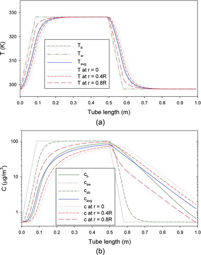
Here we assess the validity and influence of our assumption of a parabolic flow velocity profile in the TD model. Figure 1a shows that the maximum temperature deviation, at the centerline, from the bulk (plug flow) was roughly 5 K. Given this deviation between temperature fields in the plug flow and fully-developed models, we reason that the deviation of the velocity and residence time from the assumed parabolic distribution will be less than 2% (5K/300K ∼ 0.017). The entrance effect on flow field was also neglected in this study. The length and the diameter of the heating section were 58 cm and 2.2 cm, respectively, whereas those of the cooling section were 41 cm and 1.9 cm, respectively. Considering that the entrance effect lasts only for a few diameters from the entrance (∼0.07 r_t Re, according to Bird et al. 1960), it will be confined within the first 10% or so of the TD sections. As will be shown later, even the plug flow assumption does not cause a large error for MFR. Therefore, the effects of the deviation from the assumed parabolic velocity distribution due to temperature variation and entrance effects are expected to be negligible.

Figure 2a presents thermogram obtained using the present 2-D model with the experimental results of Faulhaber et al. (2009) for butanedioic acid, along with those obtained with the simpler models (“bulk temperature” and “plug flow”). The corresponding figure for hexanedioic acid (Figure S2b) looks very similar. All three sets of model results were indistinguishable for MFR above 0.2, indicating that the radial temperature and velocity distributions did not affect MFR. Apparently, deviations of temperature and velocity (relative to bulk properties) near the wall and near the tube center compensated for each other. The “plug flow” scenario resulted in the lowest MFR at high temperature and the steepest temperature dependence among all model simulations, consistent with the lack of a developed radial velocity distribution.

FIG. 2 Comparison of the measured and model-predicted MFR: (a) model differences, for butanedioic acid; (b) effect of initial aerosol concentration (C_OA), for hexanedioic acid. (Color figure available online.)

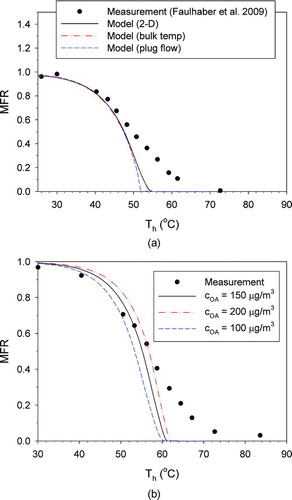
Figure 2a shows that all of the model thermograms were considerably steeper than measured ones. This observation motivated a series of sensitivity tests on the influence of model inputs on thermograms. Results discussed later are for hexanedioic acid with baseline parameters of γ _e = 1, p ⁰ = 8.86×10⁻⁶ Pa, and ΔH_v = 146.5 kJ/mol. Results from a subset of sensitivity tests are shown here; results from others are included in the online supplemental information.

Increasing the initial condensed-phase organic material concentration (c_OA ) from 150 (baseline case) to 200 μg/m³ shifts the thermograms right by 2–3° but does not affect the steepness (Figure 2b). Particle losses by diffusion or thermophoresis (Figure S3) were found to have negligible influence on the thermograms. Increasing the initial particle size (d_p ) from 200 nm (baseline case) to 220 nm has nearly the same effect on the thermogram as the concentration change (Figure S4). To assess the effect of polydispersity from the DMA classification, a 25:50:25 mixture of 180-nm, 200-nm, and 220-nm particles was simulated (Figure S4). The thermogram was slightly less steep at high temperatures than for the mono-disperse 200 nm particles, but the effect on the temperature of full evaporation was less than 1 K. It should be noted, however, that the effect of polydispersity may be considerable for aerosols not classified so narrowly. Changing the wall surface saturation (F_sat , 1 for nonadsorbing surface and 0 for perfectly adsorbing surface; F_sat = 0 for baseline) has no discernible effect on the thermogram, indicating that metal surfaces or activated carbon in any condition would work equally well for these conditions (Figure S5).

From the sensitivity runs, we conclude that uncertainties in the flow profiles, initial concentrations, particle size, or denuder surface characteristics cannot explain the discrepancy between models and measurements. We now turn to the three parameters influencing evaporation kinetics: γ _e , p_s at 25°C, and ΔH_v .

Figure 3a shows the thermograms obtained with γ _e set to 1, 0.1, and 0.01. The thermogram shifted substantially to the right and became less steep when lower values of γ _e were used.

FIG. 3 Sensitivity test results for hexanedioic acid for (a) evaporation coefficient; (b) saturation vapor pressure at 25°C; and (c) enthalpy of vaporization. (Color figure available online.)

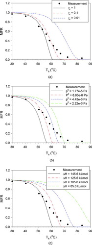
Saturation vapor pressure, determined using p_s (T_ref ), ΔH_v , and Equation (1), is the most important property dictating the evaporation rate of a material and hence the MFR result. Table 2 summarizes values of p_s (T_ref = 25°C) and ΔH_v measured by different investigators for the two dicarboxylic acids studied here. It is seen that the variation, and thus associated uncertainty, of the measured p_s (T_ref ) is more than an order of magnitude, while that of ΔH_v is relatively small. Figures 3b and c show the sensitivity of test results for values of p_s (T_ref ) and ΔH_v , respectively, reflecting uncertainty levels from literature sources. Both parameters have large influences on the thermograms. One important difference between the effects of these two parameters is that the change in p_s (T_ref ) only shifts the thermogram along the temperature axis, while change in ΔH_v affects the thermogram steepness.

TABLE 2 Summary of the values for the saturation vapor pressure at 25°C (p⁰) and the enthalpy of vaporization (ΔH_v ) reported by different investigators

				Hexanedioic acid
		Butanedioic acid
Figure 6					ΔHv
Label*	Reference	p ^0 (10^−4 Pa)	ΔHv (kJ/mol)	p ^0 (10^−5 Pa)	(kJ/mol)	Method
a	Davies and Thomas (1960)	0.423	117.4	0.842	129.4	Effusion
b	Weast (1982)	–	–	0.8	130	Effusion
c	Tao and McMurry (1989)	–	–	1.445	117.54	Kinetic
d	Chattopadhyay et al. (2001)	–	–	1.7	140	Kinetic
e	Bilde et al. (2003)	0.459	137.8	1.413	154.4	Kinetic
f	Chattopadhyay and Ziemann (2005)	1.37	119.5	3.02	146.2	Kinetic
g	Cappa et al. (2007)	0.32	128	0.26	145	Kinetic
h	Saleh et al. (2009)	3.7	88	3.4	135	Integrated volume
*Codes used in Figure 6 to identify each measurement point.

4. APPLICATION OF THE TD MODEL TO DETERMINE EVAPORATION PARAMETERS

As was discussed in the previous subsection, there are wide discrepancies between reported volatility parameters determined from TD data. We have used our detailed TD model to determine whether the discrepancies can be attributed to the use of overly simplified models (related to missing physical phenomena) or to faulty assumptions concerning the equilibria and kinetics of evaporation. Table 2 shows that all the p ⁰ values measured by the kinetic method are smaller than that suggested by Saleh et al. (2009) based on the equilibrium method. This suggests that the assumption of γ _e = 1 used for previous efforts with the kinetic method is very likely wrong. Therefore, in this subsection, we will fit the measured MFRs using different sets of γ _e , p ⁰, and ΔH_v .

The shape of a thermogram is essentially determined by the temperature at which MFR becomes 0.5 (T₅₀) and the steepness of the curve. It was shown in the previous section that γ _e and ΔH_v affect both elements, whereas p ⁰ affects the former only. In principle, we cannot simultaneously determine γ _e , p ⁰, and ΔH_v by fitting a measured thermogram with a model prediction because we have only two elements measured (T ₅₀ and the steepness) and three unknowns. If we have apriori information on one or more of the three, however, the other unknowns can be determined by fitting method as is described later.

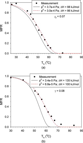
Figure 4 shows the results obtained by changing γ _e only. For p ⁰ and ΔH_v , the values suggested by Saleh et al. (2009) were used: p ⁰ = 3.7 × 10⁻⁴ Pa and ΔH_v = 88 kJ/mol for butanedioic acid and p ⁰ = 3.4 × 10⁻⁵ Pa and ΔH_v = 135 kJ/mol for hexanedioic acid. It is shown that the γ _e values suggested by Saleh et al. (2009) (0.07 ± 0.02 and 0.08 ± 0.02 for butanedioic and hexanedioic acids, respectively) lead to better agreement with measured thermograms than γ _e = 1. However, the values of γ _e that provide the best fit (0.045 and 0.03 for butanedioic and hexanedioic acids, respectively) were not within their uncertainty range. To examine the effect of the variability of experimental c_OA , Figures 4a and b show simulations conducted with c_OA = 100μg/m³ and c_OA = 200μg/m³ for the γ _e values suggested by Saleh et al. (2009). Even considering this potential variability in c_OA , the thermogram envelopes based on the γ _e values suggested by Saleh et al. (2009) do not encompass the measurements. Moreover, the steepness of the thermogram could not be matched by only changing γ _e for hexanedioic acid.

FIG. 4 Adjustment of the evaporation coefficient (γ_e) to fit the measured MFRs: (a) butanedioic acid; (b) hexanedioic acid. Also shown is the influence of variability/uncertainty in the initial aerosol concentration (C_OA) for the central values of γ_e. (Color figure available online.)

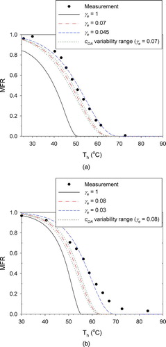
Figure 5 shows the results obtained by changing p ⁰ and ΔH_v using the γ _e values suggested by Saleh et al. (2009). For butanedioic acid, the values of p ⁰ and ΔH_v that provide the best fit (3.0 × 10⁻⁴ Pa and 86 kJ/mol) were within the uncertainty range reported by Saleh et al. (2009) ((3.7 ± 1.1) × 10⁻⁴ Pa and 88 ± 3 kJ/mol). For hexanedioic acids, however, the values of p ⁰ and ΔH_v that provide the best fit (6.8 × 10⁻⁵ Pa and 100 kJ/mol) were outside the uncertainty range reported by Saleh et al. (2009) ((3.4 ± 1.2) × 10⁻⁵ Pa and 135 ± 13 kJ/mol). Nevertheless, the overall agreement between the model prediction and measurement was much better than that obtained by only changing γ _e .

FIG. 5 Adjustment of the reference saturation pressure and the enthalpy of vaporization to fit the measured MFRs: (a) butanedioic acid; (b) hexanedioic acid. (Color figure available online.)

In the present model, all possible mechanisms have been incorporated except coagulation, which was shown to be negligible by an order-of-magnitude analysis. In addition, thorough sensitivity tests have been performed to find that influences of any uncertain parameters other than γ _e , p ⁰, and ΔH_v on thermograms are very small. There is no assumption of equilibrium or unity γ _e . Therefore, if the values of γ _e , p ⁰, and ΔH_v used in the model are accurate, the thermograms obtained by measurements should be reproduced by model prediction. Based on the results shown in Figures 4 and 5, the estimation of γ _e for both dicarboxylic acids and of p ⁰ and ΔH_v for butanedioic acid by Saleh et al. (2009) seems to be quite accurate. On the other hand, it is suggested that the estimation of p ⁰ and ΔH_v for hexanedioic acid may be less accurate.

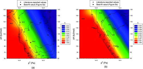
Figure 6 shows two-contour plots as functions of p ⁰ and ΔH_v for butanedioic acid (Figure 6a) and hexanedioic acid (Figure 6b): one set of contours (colored) shows the values of γ _e that give the best MFR fit while the other (lined) shows the deviation percent (DP) between model estimation and measurements for a set of γ _e , p ⁰, and ΔH_v values. Literature-reported values for p ⁰ and ΔH_v listed in Table 2 and the best-fit values obtained by fixing γ _e at the value suggested by Saleh et al. (2009) (Figure 5) are also shown. Deviation percent was defined as

where M and O represent modeled and observed values, respectively, and the overbar indicates the average. The DP values for the “best fit” results shown in Figures 5a and b were both 0.2; a better fit than this cannot be expected (Figure S6). The area having DP ≤ 0.5 is quite large in both Figures 6a and b, indicating that the three values are not constrained simultaneously with a single simulation. Nevertheless, Figure 6a demonstrates that only the (p ⁰, ΔH_v , and γ _e ) set reported by Saleh et al. (2009) (h) is within the DP ≤ 0.5 boundary. Figure 6b shows that none of the literature-reported (p ⁰, ΔH_v , and γ _e ) sets are within the DP ≤ 0.5 boundary, although the set reported by Saleh et al. is closest. Therefore, these contour plots can be a useful tool to evaluate the measured (p ⁰, ΔH_v , and γ _e ) values. By repeating the experiments under different conditions, e.g., with different TD residence times, particle concentration, and/or particle size, one can produce different contour plots. Using those contour plots collectively, the best estimation range for (p ⁰, ΔH_v , and γ _e ) will become narrower. Full application of this approach requires further development through careful design of coupled experimental and modeling studies.

FIG. 6 Contour plots for evaporation coefficient (colored) and deviation percent (contours) as functions of the reference saturation vapor pressure and the enthalpy of vaporization: (a) butanedioic acid; (b) hexanedioic acid. Literature-reported values listed in Table 2 and the best-fit values shown in Figure 5 are also shown.

5. CONCLUSIONS

Under typical conditions, the thermogram (temperature-MFR) curve from a TD simulation was shown to be remarkably insensitive to the radial variations in temperature and vapor concentration. This shows that discrepancies between published vapor pressures determined from TD experiments are unlikely due to oversimplified flow models, but are instead due to the difficulty of extracting values for the three parameters that dictate evaporation kinetics from experiments that can be fit using two-parameter models. Using the model developed here, the degree of agreement between experiments and model was examined over a wide range of evaporation coefficient (γ _e ) and other parameter values. By examining a “map” of model/measurement deviation, it was determined that the values of the parameters that provide the best fit were within the experimental uncertainty range for previous TD tests of butanedioic acid, whereas significantly better model-experiment agreement was obtained for a much lower value of enthalpy of vaporization than previously reported for hexanedioic acid. Although it appears that three-parameter fitting can be facilitated by appropriate TD models, the results will depend on experimental errors, which are difficult to quantify for measurements in the literature.

Acknowledgments

Funding from the Natural Sciences and Engineering Research Council of Canada is appreciated.

[Supplementary materials are available for this article. Go to the publisher's online edition of Aerosol Science and Technology to view the free supplementary files.]

REFERENCES

- An , W. J. , Pathak , R. K. , Lee , B.-H. and Pandis , S. N. 2007 . Aerosol Volatility Measurement Using an Improved Thermodenuder: Application to Secondary Organic Aerosol . J. Aerosol Sci. , 38 : 305 – 314 .
- Bilde , M. , Svenningsson , B. , Monster , J. and Rosenorn , T. 2003 . Even-odd Alternation of Evaporation Rates and Vapor Pressures of C3–C9 Dicarboxylic Acid Aerosols . Environ. Sci. Technol. , 37 : 1371 – 1378 .
- Bird , R. B. , Stewart , W. E. and Lightfoot , E. N. 1960 . Transport Phenomena , New York : Wiley .
- Cappa , C. D. 2010 . A Model of Aerosol Evaporation Kinetics in a Thermodenuder . Atmos. Meas. Tech. , 3 : 579 – 592 .
- Cappa , C. D. , Lovejoy , E. R. and Ravishankara , A. R. 2007 . Determination of Evaporation Rates and Vapor Pressures of Very Low Volatility Compounds: A Study of the C-4-C-10 and C-12 Dicarboxylic Acids . J. Phys. Chem. A , 111 : 3099 – 3109 .
- Cappa , C. D. and Wilson , K. R. 2011 . Evolution of Organic Aerosol Mass Spectra Upon Heating: Implications for OA Phase and Partitioning Behavior . Atmos. Chem. Phys. , 11 : 1895 – 1911 .
- Chapman , S. and Cowling , T. G. 1970 . The Mathematical Theory of Non-uniform Gases , Cambridge : Cambridge University Press .
- Chattopadhyay , S. , Tobias , H. J. and Ziemann , P. J. 2001 . A Method for Measuring Vapor Pressures of Low-volatility Organic Aerosol Compounds Using a Thermal Desorption Particle Beam Mass Spectrometer . Anal. Chem. , 73 : 3797 – 3803 .
- Chattopadhyay , S. and Ziemann , P. J. 2005 . Vapor Pressures of Substituted and Unsubstituted Monocarboxylic and Dicarboxylic Acids Measured Using an Improved Thermal Desorption Particle Beam Mass Spectrometry Method . Aerosol Sci. Technol. , 39 : 1085 – 1100 .
- Davies , M. and Thomas , G. H. 1960 . The Lattice Energies, Infra-red Spectra, and Possible Cyclization of Some Dicarboxylic Acids . Trans. Faraday Soc. , 56 : 185 – 192 .
- Faulhaber , A. E. , Thomas , B. M. , Jimenez , J. L. , Jayne , J. T. , Worsnop , D. R. and Ziemann , P. J. 2009 . Characterization of a Thermodenuder-Particle Beam Mass Spectrometer System for the Study of Organic Aerosol Volatility and Composition . Atmos. Meas. Tech. , 2 : 15 – 31 .
- Fierz , M. , Vernooij , M. G. C. and Burtscher , H. 2007 . An Improved Low-Flow Thermodenuder . J. Aerosol Sci. , 38 : 1163 – 1168 .
- Fuchs , N. A. and Sutugin , A. G. 1971 . “ High-Dispersed Aerosols ” . In Topics in Current Aerosol Research , Edited by: Hidy , G. M. and Brock , J. R. 1 – 60 . New York : Pergamon Press .
- Gelbard , F. 1990 . Modeling Multi-component Aerosol Particle Growth by Vapor Condensation . Aerosol Sci. Technol. , 12 : 399 – 412 .
- Grieshop , A. P. , Donahue , N. M. and Robinson , A. L. 2007 . Is the Gas-Particle Partitioning in Alpha-Pinene Secondary Organic Aerosol Reversible? . Geophys. Res. Lett. , 34 : L14810 doi: 14810.11029/12007GL029987
- Grieshop , A. P. , Miracolo , M. A. , Donahue , N. M. and Robinson , A. L. 2009 . Constraining the Volatility Distribution and Gas-Particle Partitioning of Combustion Aerosols Using Isothermal Dilution and Thermodenuder Measurements . Environ. Sci. Technol. , 43 : 4750 – 4756 .
- Hinds , W. C. 1999 . Aerosol Technology: Properties, Behavior, and Measurements of Airborne Particles , 2nd Ed. , New York : John Wiley & Sons .
- Kim , Y. P. and Seinfeld , J. H. 1990 . Simulation of Multicomponent Aerosol Condensation by Moving Sectional Method . J. Colloid and Interf. Sci. , 135 : 185 – 199 .
- Kulmala , M. and Wagner , P. E. 2001 . Mass Accommodation and Uptake Coefficients—A Quantitative Comparison . J. Aerosol Sci. , 32 : 833 – 841 .
- Li , W. G. and Davis , E. J. 1996 . Aerosol Evaporation in the Transition Regime . Aerosol Sci. Technol. , 25 : 11 – 21 .
- Monster , J. , Rosenorn , T. , Svenningsson , B. and Bilde , M. 2004 . Evaporation of Methyl- and Dimethyl-substituted Malonic, Succinic, Glutaric and Adipic Acid Particles at Ambient Temperatures . J. Aerosol Sci. , 35 : 1453 – 1465 .
- Park , D. , Kim , S. , Choi , N. K. and Hwang , J. 2008 . Development and Performance Test of a Thermo-denuder for Separation of Volatile Matter From Submicron Aerosol Particles . J. Aerosol Sci. , 39 : 1099 – 1108 .
- Press , W. H. , Flannery , B. P. , Teukolsky , S. A. and Vetterling , W. T. 1989 . Numerical Recipes: The Art of Scientific Computing (Fortran Version) , New York : Cambridge University Press .
- Rader , D. J. and McMurry , P. H. 1986 . Application of the Tandem Differential Mobility Analyzer to Studies of Droplet Growth and Evaporation . J. Aerosol Sci. , 17 : 771 – 787 .
- Riipinen , I. , Pierce , J. R. , Donahue , N. M. and Pandis , S. N. 2010 . Equilibration Time Scales of Organic Aerosol Inside Thermodenuders: Evaporation Kinetics Versus Thermodynamics . Atmos. Environ. , 44 : 597 – 607 .
- Riipinen , I. , Svenningsson , B. , Bilde , M. , Gaman , A. , Lehtinen , K. and Kulmala , M. 2006 . A Method for Determining Thermophysical Properties of Organic Material in Aqueous Solutions: Succinic Acid . Atmos. Res. , 82 : 579 – 590 .
- Saleh , R. , Khlystov , A. and Shihadeh , A. 2011a . Determination of Evaporation Coefficients of Ambient and Laboratory-generated Semivolatile Organic Aerosols From Phase Equilibration Kinetics in a Thermodenuder . Aerosol Sci. Technol. , 46 : 22 – 30 .
- Saleh , R. and Shihadeh , A. 2007 . Hygroscopic Growth and Evaporation in an Aerosol with Boundary Heat and Mass Transfer . J. Aerosol Sci., , 38 : 1 – 16 .
- Saleh , R. , Shihadeh , A. and Khlystov , A. 2009 . Determination of Evaporation Coefficients of Semi-volatile Organic Aerosols Using an Integrated Volume-Tandem Differential Mobility Analysis (IV-TDMA) Method . J. Aerosol Sci. , 40 : 1019 – 1029 .
- Saleh , R. , Shihadeh , A. and Khlystov , A. 2011b . On Transport Phenomena and Equilibration Time Scales in Thermodenuders . Atmos. Meas. Tech. , 4 : 571 – 581 .
- Saleh , R. , Walker , J. and Khlystov , A. 2008 . Determination of Saturation Pressure and Enthalpy of Vaporization of Semi-volatile Aerosols: The Integrated Volume Method . J. Aerosol Sci. , 39 : 876 – 887 .
- Seinfeld , J. H. and Pandis , S. N. 1998 . Atmospheric Chemistry and Physics: From Air Pollution to Climate Change , New York : John Wiley & Sons .
- Stanier , C. O. , Pathak , R. K. and Pandis , S. N. 2007 . Measurement of the Volatility of Aerosol From α-pinene Ozonolysis . Environ. Sci. Technol. , 41 : 2756 – 2763 .
- Tao , Y. and McMurry , P. H. 1989 . Vapor Pressures and Surface Free Energies of C14–C18 Monocarboxylic Acids and C5 and C6 Dicarboxylic Acids . Environ. Sci. Technol. , 23 : 1519 – 1523 .
- Thalladi , V. R. , Nusse , M. and Boese , R. 2000 . The Melting Point Alternation in α-ω-alkanedicarboxylic Acids . J. Am. Chem. Soc. , 122 : 9227 – 9236 .
- Vaden , T. D. , Imre , D. , Beranek , J. , Shrivastava , M. and Zelenyuk , A. 2011 . Evaporation Kinetics and Phase of Laboratory and Ambient Secondary Organic Aerosol . Proc. Nat. Acad. Sci. USA , 108 : 2190 – 2195 .
- Virtanen , A. , Joutsensaari , J. , Koop , T. , Kannosto , J. , Yli-Pirila , P. Leskinen , J. 2010 . An Amorphous Solid State of Biogenic Secondary Organic Aerosol Particles . Nature , 467 : 824 – 827 .
- Weast , R. C. 1982 . Handbook of Chemistry and Physics , Boca Raton, FL : CRC Press .
- Zhang , S.-H. , Seifeld , J. H. and Flagan , R. C. 1993 . Determination of Particle Vapor Pressures Using the Tandem Differential Mobility Analyzer . Aerosol Sci. Technol. , 19 : 3 – 14 .