A Portable High-Resolution Polar Nephelometer for Measurement of the Angular Scattering Properties of Atmospheric Aerosol: Design and Validation

Abstract

The light-scattering properties of atmospheric aerosol particles are important for understanding their effects on Earth's climate, remote sensing studies of particulate matter, and visibility studies. However, aerosol optical properties are relatively poorly understood and have been identified as one of the largest uncertainties in our understanding of anthropogenic effects on climate. Direct in situ and laboratory studies of aerosol light-scattering may help reduce these uncertainties and improve remote sensing studies. A field-deployable, high angular resolution polar nephelometer has been developed for the measurement of the scattering properties of aerosol particles. The instrument utilizes an elliptical mirror, laser, and charge-coupled device camera to measure the aerosol angular scattering intensity (phase function) and degree of linear polarization (polarization ratio) across an angle range of 20°–155° at a resolution as high as 0.31°–0.59° per pixel. The instrument design was validated by laboratory measurements of the scattering properties of polystyrene latex (PSL) microspheres at a wavelength of 532 nm and comparison with Lorenz–Mie theory. The instrument accurately measured the predicted phase function and linear polarization for four sizes of monodisperse PSL with diameters ranging from 300 to 750 nm, except for very narrow features predicted by the theory. The instrument offers high angular resolution and the capability to measure multiple angles simultaneously. Advantages and disadvantages of the technique are discussed.

© 2013 American Association for Aerosol Research

1. INTRODUCTION

The optical properties of aerosol particles determine how they scatter and absorb light in the atmosphere, in turn affecting Earth's radiation budget and global climate. The scattering of incoming and outgoing light has been termed the direct effect of aerosols on climate. However, the optical properties of atmospheric aerosol particles are relatively poorly understood and have been identified as one of the largest uncertainties in our understanding of climate (Forster et al. 2007; Solomon et al. 2007). The spectroscopic properties of aerosol particles are also used in the interpretation of remote sensing measurements of the atmosphere from satellite, aircraft, and ground-based systems. Aerosol light scattering also affects air quality and visibility in the atmosphere. Direct in situ and laboratory measurements of the scattering properties of aerosols may help reduce uncertainties in climate and remote sensing studies.

When light encounters an aerosol in the atmosphere, the incident light may be attenuated through scattering, absorbance, or both. Scattering depends on the complex refractive index of the material composing the particles, mixing state if there is more than one component, the size and shape of the particles, and the orientation of the particles if they are not spherical. Scattering by an ensemble of particles spaced relatively far apart (eliminating multiple scattering) is explicitly described by the 4 × 4 scattering matrix transformation of the Stokes parameters of the incident light (van de Hulst 1957; Bohren and Huffman 1983; Mishchenko et al. 2002).

The scattering phase function is one element of the scattering matrix (element F ₁₁) and is a measure of the intensity of scattered light from a particle as a function of scattering angle. Typically, this is presented in a normalized, dimensionless form of relative scattering intensity for unpolarized incident light as a function of scattering angle, θ, where θ = 0° represents complete forward scattering and θ = 180° represents complete backward scattering. Another useful quantity, the degree of linear polarization (ratio of elements: F ₁₂/F ₁₁), also referred to as the polarization ratio, describes how different polarizations of incident light scatter in relation to one another (van de Hulst 1957; Bohren and Huffman 1983; Mishchenko et al. 2002).

Particles with a diameter approximately equal to the wavelength of scattered light are said to be in the Mie scattering regime and are commonly found in Earth's atmosphere (Seinfeld and Pandis 2006). Scattering by spherical particles in the Mie regime is well understood via Lorenz–Mie theory, so a measurement of the phase function of such particles can be used to determine their size or refractive index (Barkey et al. 2007; Castagner and Bigio 2007; Kim et al. 2010). Scattering by irregularly shaped particles is more complex, but two major methods have been developed, the T-matrix method and discrete dipole approximation, to better describe such scattering (Draine and Flateau 1994; Mishchenko et al. 1996, 2002; Dubovik et al. 2002).

Several laboratory and field instruments have been developed for the study of the angular scattering properties of aerosol particles and cloud water or ice droplets. Some of these instruments will be discussed here only briefly, and we refer the reader to the recent review by Muñoz and Hovenier (2011) for more discussion, particularly in regard to nonspherical particles. In general, these methods involve scattering laser light from an ensemble of particles and measuring scattering intensity as a function of scattering angle, hence these instruments have been called polar nephelometers. Scattering is typically measured for different rotational positions of the laser polarization that is incident on the aerosol to obtain the linear polarization and other scattering matrix elements. The scattering for different incident polarizations can be summed to obtain the angular scattering intensity for unpolarized incident light.

Several strategies have been used for polar nephelometers. These include mounting a photomultiplier tube (PMT) detector on an arm that moves through the scattering angles (Munoz et al. 2001; Volten et al. 2001; Liu et al. 2003; Muñoz et al. 2010; Muñoz and Hovenier 2011), mounting multiple photodiode detectors at several angles around the particles (Gayet et al. 1997, 1998; West et al. 1997; Barkey and Liou 2001; Barkey et al. 2002, 2007), using parabolic and moving mirrors to scan across angles onto a PMT (Castagner and Bigio 2006, 2007), and using an ellipsoidal mirror to direct scattered light through a rotating tube to a PMT (Kaller 2004).

Recently, a laboratory-scale instrument was developed that uses an elliptical mirror to reflect scattered light onto a charge-coupled device (CCD) linear array detector (Curtis et al. 2007, 2008; Meland et al. 2011, 2012). The elliptical mirror and CCD detector method offers high angular resolution and relatively fast measurement times without moving parts except for a rotator to control the laser incident polarization. The method also has the ability to measure a wide range of scattering angles simultaneously, without the need for multiple detectors or a movable detector.

The above instruments, with one exception to our knowledge, have been restricted to either laboratory measurements of aerosol properties or field measurements of larger cloud droplets or ice particles. Only the Barkey et al. (2007) instrument has been both portable and sensitive enough to be used for field-based aerosol studies and was recently used to measure scattering properties of aerosol from a smog chamber exposed to ambient sunlight (Kim et al. 2010). (It should be noted that the Kaller (2004) instrument could likely be used in this capacity, but has not been deployed, to our knowledge. In addition, the other sensitive methods, such as the moving arm-mounted PMT, could possibly be adapted to field use.) The Barkey et al. (2007) instrument is based on mounting multiple photodiode detectors in an array around the scattering region and requires calibration of each detector individually.

For the current study, a miniaturized, field-deployable, polar nephelometer was developed based on the elliptical mirror method laboratory-scale instrument developed by Curtis et al. (2007). The instrument design and alignment was validated by measuring the phase function and linear polarization of various sizes of polystyrene latex (PSL) microspheres at a wavelength of λ = 532 nm and by comparing the measured data to the expected scattering properties calculated from Lorenz–Mie theory. One size of PSL (diameter of D _p = 600 nm) was used to align the instrument and determine a calibration response function for the detector. The calibration was then applied to measurements for the other sizes. After calibration, good agreement was observed between the measured and theoretical phase function and linear polarization for each size of PSL. The portable instrument provides a higher signal to noise ratio and more accurate results than the laboratory instrument in a shorter exposure time.

2. EXPERIMENTAL METHOD

2.1. Scattering Apparatus

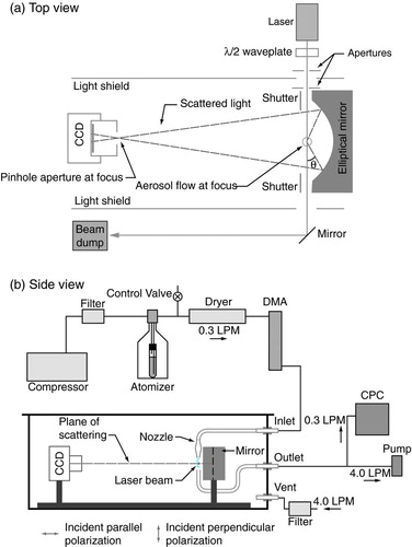
Figure 1 shows a schematic diagram of the instrument, with the top panel (a) showing a top view detail of the elliptical mirror, laser, and CCD system and the bottom panel (b) illustrating a side view of the aerosol inlet and outlet, plane of scattering, and the two incident polarizations used in relation to the plane of scattering. The apparatus was assembled in a custom-built black polyethylene container in order to minimize stray light reaching the detector. The inside walls of the container were roughly sanded and painted with flat black paint to reduce reflection of stray light. The top lid of the container was removable and held in place with a clamp at each corner. The top edges of the container had a rubber gasket to allow the lid to be sealed when clamped. The container was sealed by silicone on all screws, edges, and wiring passing through the walls in order to allow ambient air to be pulled into a sample inlet by an external pump attached to an outlet. The walls of the container had a thickness of approximately 1 cm, which reduced deformations of the container when pulling a slight vacuum with the pump.

FIG. 1 Top (a) and side (b) schematic views of the experimental apparatus based on an elliptical mirror. Particles scattered laser light from one focus of the ellipse and the light was focused through a pinhole aperture onto a linear CCD. Flow rates are indicated with arrows in liters per minute (LPM). DMA = differential mobility analyzer, CPC = condensation particle counter. (Color figure available online.)

The container had dimensions of 74.5 cm × 74.5 cm × 24.5 cm resulting in a contained volume of approximately 13.6 L. In principle, the container could be made smaller, as the actual scattering apparatus is smaller, but for initial tests of the instrument, a larger size was desired to allow space for alignment and to create an entirely self-contained unit. In this form, the laser, laser power supply, and all optical components were placed inside the container. If a smaller size were required, the laser power supply could be placed outside of the container and other unused space could be eliminated. An optical breadboard (Newport Corp.) was attached to the floor of the box for secure placement of components. Any light-generating components inside the container, such as the liquid crystal display (LCD) on the laser power supply, were covered with black tape to prevent stray light from reaching the detector.

The major optical components were a laser, elliptical mirror, λ/2 waveplate, and CCD camera used as a detector. Each component is described in detail below. The principles of light scattering from an aerosol onto an elliptical mirror and focusing of the light onto a CCD camera have been discussed previously (Curtis et al. 2007; Meland 2011) and are described here only briefly. The laser beam passed in front of the face of the elliptical mirror and through an aerosol flow region placed at one focus of the ellipse describing the mirror shape. Any light scattered from the aerosol to the elliptical mirror must be refocused onto the second focus of the ellipse defining the shape of the mirror. A pinhole aperture was placed at the second focus, and the scattered light was subsequently detected with the CCD array detector. The distance between the foci of the ellipse (the location of the aerosol and the pinhole aperture) was designed as 18.8 cm and the CCD detector was approximately 1 cm from the pinhole. The pinhole aperture had a diameter of 500 μm (Edmund Optics Part NT39-729) and was attached to a larger aperture attached to the camera's threaded filter mount. The scattering angle of light from the aerosol was determined based on where the light hit the linear CCD using an angle calibration protocol described below. The intensity was determined from the normalized relative signal detected at each pixel of the CCD during a 10-s exposure of the camera after applying an intensity calibration to account for sensitivity variation across the detector.

A green diode-pumped solid-state continuous-wave (CW) laser with a wavelength of λ = 532 nm (model CL532-050-LO, Crystalaser) was used as the light source in this study. This wavelength is commonly used in spectroscopic studies due to its proximity to the solar maximum wavelength and is the wavelength of the commonly used frequency-doubled Nd:YAG laser. The laser was powered by an adjustable power supply set at 40 mW. The laser was linearly polarized at a ratio of >50:1, according to the manufacturer. The light passed through a λ/2 waveplate used to control the direction of polarization of the laser beam incident to the aerosol. The waveplate rotational position was software-controlled by a computer connected to a rotation stage (model CONEX-AG-PR100P, Newport, Inc.) to better than one degree of resolution. In this study, two incident polarization states were studied, parallel to the measured plane of scattering and perpendicular to the measured plane of scattering (often referred to as the p and s orientations, respectively), allowing the degree of linear polarization to be determined, as described below. Tests were performed to optimize the rotational angle of the waveplate and thus the polarization state of the incident light, by rotating the waveplate in one degree increments and measuring the scattered light from PSL. The polarization state of the scattered light was not determined in this study but could be with the addition of a polarizing filter in front of the detector.

The laser beam passed in front of a custom-built mirror based on the shape of an ellipse (Custom Scientific, Inc.). Light scattered from the aerosol was reflected from the mirror and focused through a pinhole aperture onto a CCD camera (model ST-402ME, Santa Barbara Instruments Group). The camera was Peltier-cooled to approximately 2.5°C to help reduce thermal noise. The mirror had a width of approximately 10.7 cm, including 2.0 cm of flat face on each side. The shape of the mirror face was based on an ellipse with a major axis of 24.0 cm and a minor axis of 15.0 cm. The mirror flat face was designed to start 4.0 mm from the focus to allow room for the laser to pass in front of the mirror. The mirror had a pinhole though the front face that was used for alignment during initial setup, but this pinhole was placed above the plane of scattering and did not affect the particle measurements.

One limitation of all nephelometers is that the light scattered at 0° and 180° cannot be detected due to the need to steer the light to the aerosol. The movable-arm method has reduced this dead area to 3° at best on each side, resulting in measuring the angular scattering from a range of approximately 3°–177° (Muñoz et al. 2010). Other polar nephelometers have reported angular scattering ranges of 5°–175° (Barkey and Liou 2001), 15°–175° (Curtis et al. 2007), 15°–170° (West et al. 1997), 10°–160° (Kaller 2004), and 70°–125° (Castagner and Bigio 2007). For the elliptical mirror method, the laser beam requires a few millimeters to pass in front of the face of the mirror. Also, stray light from the laser beam can hit the flat face of the mirror, particularly the corners where the elliptical face begins, and be detected as very bright interference on the CCD. These effects further reduce the scattering angle range that can be measured at the forward and backward extremes. To reduce the flat mirror reflections in this study, two apertures were placed in the laser beam path to reduce stray light and shutters were placed between the mirror and the CCD to prevent remaining stray light from reaching the detector (Curtis et al. 2007). For the instrument described here, the expected angle range based on the mirror geometry was approximately 6°–174°, but the effective scattering angle range that could be detected was reduced to approximately 20°–155°. Beyond that angle range, the shutters blocked the light. Further efforts are being performed to improve the scattering angle range.

It is important to note that the light reaching the detector was not scattered from an infinitely small volume of the aerosol but likely reached the detector from multiple regions in the scattering volume, based on the size of the pinhole aperture in front of the camera and the width of the laser beam (Meland 2011). The laser beam had a Gaussian width of approximately 0.36 mm (twice the radius from the center of the beam to a distance at which the intensity decreases by a factor of 1/e²) and the aerosol nozzle had a 2.5 mm opening, leading to a scattering volume shaped like a rectangle with a width of approximately 2.5 mm along the face of the mirror. The pinhole aperture in front of the CCD camera blocked light scattered from most of the other regions within the aerosol that were not on the mirror focus. However, light scattered from the aerosol directly to the camera at 90° without reflecting from the mirror was detected. This light was observed by covering the mirror with a piece of black felt cloth and subtracted from the images where the mirror was exposed. We refer to these measurements as “direct images” to indicate that the light observed did not reflect from the mirror. Any other stray light was also subtracted by measuring light scattering without PSL particles and we refer to these as “blank images.” The direct scatter and blank subtraction method is described in detail below.

In order to increase the signal to noise ratio, the CCD camera pixels were binned in a 3 × 3 matrix. Therefore, the detector had an actual size of 1530 × 1020 pixels, but binning reduced the effective pixel number to 510 × 340. In practice, the CCD-captured scattering region was 135° spread across 267 pixels, resulting in an angular resolution ranging from 0.31° per pixel at the edge of the image to 0.59° per pixel at the center of the image, after binning. Without binning, the angular resolution could be improved by a factor of three, but with increased noise.

Fine alignment of the beam, mirror, and camera system was performed by measuring scattering intensity for both polarizations from PSL particles with a diameter of D _p = 600 nm (5000 series, Thermo Scientific). PSL particles have been heavily used in aerosol optical studies and are well characterized and spherical in shape, thus providing convenient test particles for scattering instruments (West et al. 1997; Castagner and Bigio 2006, 2007; Barkey et al. 2007; Curtis et al. 2007; Kim et al. 2010). The measured angular intensities and linear polarization were compared with the expected angular intensities and linear polarization calculated from a Lorenz–Mie theoretical model for monodisperse spherical particles based on BHMIE in Bohren and Huffman (1983).

The refractive index of PSL was recently measured to be n = 1.60 ± 0.02 and k = 0.01 ± 0.03 at λ = 532 nm (Lang-Yona et al. 2009). The values n = 1.60 and k = 0.00 were used in this study as the refractive index for alignment purposes, with uncertainties discussed below. The system was aligned such that the general shape of the measured angular intensities and linear polarization was matched to the theory. An angle calibration procedure was performed to map the pixels from the images to the scattering angles in degrees. The angle calibration procedure is described in detail below. Additional elements of the scattering matrix were not measured in this study, but could be determined with the addition of a polarizer in front of the detector. During a field campaign, it is expected that the instrument would be prealigned and calibrated in the laboratory and that the alignment would be periodically calibrated with PSL or another aerosol with known optical properties.

2.2. Particle Generation

An aerosol of dried PSL particles was generated from diluted suspensions using a constant output atomizer (model 3076, TSI, Inc.) and diffusion dryer (model 3062, TSI, Inc.). The relative humidity of the dried aerosol was measured to be 10%–20%. The purchased PSL microspheres were in an aqueous suspension, which was diluted for atomization in Milli-Q water (18 MΩ·cm resistivity) at a ratio of approximately 0.1 mL of PSL suspension to 9 mL of water. The diluted suspension was placed in a plastic test tube, sealed, and sonicated for approximately 60 s prior to atomization.

The atomizer tube and drain tube were placed through a plastic stopper into the test tube and the entire test tube assembly was placed in the vacuum-sealed glass flask generally used for this atomizer. The test tube setup was used in order to obtain relatively high concentrations of PSL while using small amounts of the PSL suspension, as the atomizer generates the aerosol from a volume of approximately 9 mL rather than the large flask, which requires a suspension volume of at least approximately 300 mL. One disadvantage of this method is that the PSL concentration in the diluted suspension can vary more quickly than when using a larger volume. For this study, the number density of the aerosol was carefully monitored with a condensation particle counter (CPC) (model 3775, TSI, Inc.) during the scattering measurements to ensure that the number density was constant, within the error of the instrument. Care was taken to ensure that particle concentrations in the diluted suspensions were low enough that particle coagulation was minimized and less than one particle, on average, was present per droplet produced by the atomizer. Even so, the particles were size-selected as described below.

The PSL suspension as ordered from the manufacturer contained a small amount of surfactant in order to keep the particles from coagulating in the suspension. The surfactant was diluted along with the PSL in the suspension, but it is possible that a small amount of surfactant remained on the particles after drying (Pettersson et al. 2004). The possibility of surfactant on the surface was ignored in this study for the size selection, scattering measurement, and Lorenz–Mie model calculations.

Although the PSL was highly monodisperse as purchased (3% CV width, according to the manufacturer), the aerosol was size-selected using the differential mobility analyzer (DMA) prior to imaging with the nephelometer. The DMA sheath flow was carefully monitored to be 10 times the aerosol flow rate of 0.3 liters per minute (LPM), which was controlled by a bleed valve between the atomizer and dryer. Size-selection ensured the removal of any clusters or remaining wet particles from the aerosol, which would scatter light very efficiently. The dried size-selected PSL aerosol was then allowed to pass through conductive tubing to the nephelometer inlet.

FIG. 2 Scattering images for PSL with a diameter of D _p = 600 nm with parallel polarization. Image 1 shows light from PSL and room air scattered from the mirror surface. Image 2 shows light from room air only scattered from the mirror surface. Image 3 shows light from PSL and room air scattered directly to the camera with the mirror covered. Image 4 shows light from room air only scattered directly to the camera with the mirror covered. The lines in Image 1 indicate the vertical range of summation used to determine intensity. See text for details.

In order to ensure aerosol flow across the scattering region from the nozzle to the outlet, air was pumped from the box at a flow rate of 4.0 LPM by a compact battery-powered portable sampling pump (Gilian 5000, Sensidyne). An additional 0.3 LPM was pulled by the CPC. Make-up air was allowed to flow into the box through a high-efficiency particulate air (HEPA) filter in order to equilibrate the pressure in the box. The flow rate of the make-up air was measured to be 4.0 LPM with a bubble-type flow meter (Gilibrator, Sensidyne), indicating minimal air leakage into the box from other locations. The flow rate out of the instrument was high enough to constrain the aerosol to move directly from the nozzle to the outlet without spreading in the box, as confirmed visually. The background number density in the box was approximately 20 cm⁻³ prior to introducing the PSL, indicating that the room air particles, with a typical measured number density up to 2000 cm⁻³, were effectively filtered. With a flow rate of 0.3 LPM exiting the nozzle, the airflow is expected to be laminar. It is unclear what effect laminar flow would have on the orientation of nonspherical particles, but for this study, the particles are spherical and the orientation does not matter.

Lorenz–Mie theory assumes that the particles are far enough apart that light is only singly scattered such that each particle acts independently. The range of values of the measured number density of PSL during scattering measurements was approximately 100 cm⁻³ (for 750 nm PSL) to 1.8 × 10³ cm⁻³ (for 300 nm PSL), well below the concentrations required to obtain multiple scattering, even when accounting for dilution by the make-up air (Mishchenko et al. 2002).

During measurements of ambient particles, a slightly different configuration will be used once the instrument has been aligned using PSL. The vent will be closed so that particles are pulled into the box by the pump through the inlet from ambient air. If desired, the ambient particles could be size-selected by the DMA, but more likely the DMA will be placed directly before the CPC in the scanning mobility particle sizer (SMPS) configuration to determine the size distribution of the ambient particles. For the present study, attempts were made to produce PSL aerosol and monitor the size distribution in this manner. However, the SMPS was not able to accurately measure the very narrow size distribution of the PSL, as was also noted in Barkey et al. (2007).

2.3. Data Processing Protocol and Background Correction

For each incident polarization, four imaging conditions were used to correct for background scattering and stray light: (1) scattering from the mirror with PSL entering the instrument (“scattering”), (2) scattering from the mirror with only filtered room air entering the instrument (“blank”), (3) scattering directly from the scattering region to the CCD with the mirror covered with PSL entering the instrument (“direct”), and (4) scattering directly from the scattering region to the CCD with the mirror covered with only filtered room air entering the instrument (“blank direct”). Each image in this study had an exposure time of 10 s. For each set of conditions, three images were collected and averaged to reduce noise. The images were averaged prior to any normalization, but could be normalized prior to averaging if the particle number density was highly variable. We refer to the averaged images collected under these four conditions as Image 1, Image 2, Image 3, and Image 4, respectively. Each individual image had a dark frame subtracted that was collected automatically by the camera by closing a shutter directly in front of the sensor. The dark frame accounted for any thermal noise at the detector. If required, the exposure time could be increased for ambient studies, with reduced temporal resolution. More sensitive CCD cameras are also available and could be substituted fairly easily at increased cost.

The four averaged images were collected for each incident polarization of the laser. Figure 2 shows the set of scattering images for parallel polarized incident light for 600 nm PSL. Figure 3 shows the set of scattering images for perpendicular polarized incident light for 600 nm PSL. In Figures 2 and 3, the upper left panel shows Image 1 (scattering), the upper right panel shows Image 2 (blank), the lower left panel shows Image 3 (direct), and the lower right panel shows Image 4 (blank direct). All images in Figures 2 and 3 are shown with the same intensity scale and can be directly compared with one another, but Images 2–4 have been multiplied by a factor of 10 to be able to observe the small signals in those images.

FIG. 3 Scattering images for PSL with D _p = 600 nm as in Figure 2 but with perpendicular polarization.

FIG. 4 CPC number density measurement as a function of time for the images shown in Figures 2 and 3 for PSL with D _p = 600 nm. The gray areas indicate the times at which the four images were taken. The large spike in number density occurred when the box was opened to cover the mirror. Note that the two blank measurements had the same number density and that the two particle measurements (scattering and direct) had the same number density. The perpendicular and parallel images were measured immediately in succession within minutes with identical number density.

In Figure 2, it can be seen that Image 1 is the brightest of the four, as would be expected. Image 3 shows the scattered light directly from PSL with the mirror covered. We attribute the bright spot near the center of the image to light scattered directly from the PSL at 90°. Very little intensity can be seen in Image 4, the direct scattering without PSL present.

Figure 3 shows similar behavior for the perpendicular polarization. However, in Image 1, more structure can be seen than in Image 1 in Figure 2. This pattern is expected from Lorenz–Mie theory and will be discussed below. The other major difference between Figures 2 and 3 is that direct scattering was observed across a wider horizontal range. We attribute this to Rayleigh scattering from the gas molecules in the air, which is expected to be higher for the perpendicular polarization, as parallel polarized light is Rayleigh scattered less efficiently than perpendicular except at 0° and 180° (Bohren and Huffman 1983).

The particle number density was closely monitored with the CPC while the images were being collected to ensure consistency. Figure 4 illustrates the number density measurement for the images shown in Figures 2 and 3. The gray regions indicate the approximate time when the images were collected. The number density did not change, within the noise of the CPC, while the three individual images were collected prior to averaging. The number density was also identical for the parallel and perpendicular incident polarizations collected for each set of images. The box was opened between Image 2 and Image 3, at approximately 66 min in order to cover the mirror, which greatly increased the particle number density in the box. The box was closed and filtered air was pulled into the inlet for enough time to return to the background number density (typically 60 min) before measuring the blank direct images. The number density for the direct scattering measurement was the same as for the scattering image with the mirror uncovered so that the direct scattering was correctly subtracted. The small spikes in intensity before and after adding the particles were caused by a small intake of room air when changing the configuration.

To determine the total intensity observed across the scattering angle range for each image, the intensity of each pixel was summed between pixel rows 135–175 for each column of pixels from 1–510. Figures 2 and 3 illustrate the summation range in the panel for Image 1 as white lines on the left side of the image. It can be seen that the range includes the entire vertical extent of the scattered light. The resulting summed intensity was designated I ₁, I ₂, I ₃, and I ₄, for Images 1–4, respectively. The scattering intensity for the PSL particles was determined by subtracting the intensity for blank images and direct images from the intensity from Image 1 as:

where Polarization is designated as Para for parallel incident polarization and Perp for perpendicular incident polarization, such that I _para is the resulting scattering intensity from PSL for parallel incident polarization after background corrections and averaging and I _perp is the resulting scattering intensity from PSL for perpendicular polarization after background corrections and averaging. These designations refer to the polarization of the incident laser only, as the polarization state of the scattered light was not determined in this study. The subtraction procedure removes the effects of direct scattering, scattering from background stray light, and Rayleigh scattering such that the resulting intensity is only from light scattered from PSL particles from the mirror.

The total phase function is defined as

where I _Total, I _Perp, and I _Para were normalized to the theoretical scattering intensities in order to allow direct comparison between the measured and theoretical values as described in detail in Section 2.5. These designations for the normalized values are used for the remainder of this manuscript.

Tests were performed with the 600 nm PSL to ensure that the detector was not saturated at the intensities measured and exposure times used in this study. The maximum detector response was linear for an exposure time ranging from 1 to 20 s, for both the parallel and perpendicular incident polarizations. Maximum intensities for the other sizes were within the linear range. Blooming of the CCD was not observed at the maximum intensities measured for any size. Additional tests were performed to determine any differences in the sensitivity of the CCD to varying polarizations of light striking the detector itself. The laser beam was directed directly into the CCD (through multiple neutral density filters) by a flat mirror placed in the beam. The signal was monitored while the waveplate rotated the beam through all polarizations. A small variation of approximately 5% was observed in the intensity. This was approximately on the order of the combined uncertainty from the images and calibration described below but was not considered in the uncertainty.

2.4. Angle Calibration Procedure

In order to convert the horizontal scale of the image from pixels to scattering angle, the following calibration procedure was performed for all sizes of PSL and is illustrated for 600 nm PSL here. Because the linear polarization shows well-resolved structure and accounts for each incident polarization, it was used to calibrate the pixel number to correspond to a specific scattering angle. The degree of linear polarization (scattering polarization ratio) is defined as

and was calculated for the measured intensities as a function of horizontal pixel number.

Based on the measured linear polarization (plotted as a function of pixel number) and the theoretical linear polarization (determined as a function of scattering angle in degrees), a calibration function was determined to map the pixels onto specific angles. For all sizes of PSL, the measured and calculated linear polarizations had clear regions of high and low values. Figure 5 illustrates the calibration method by showing the plots of measured linear polarization as a function of pixel number (top) and the theoretical linear polarization as a function of scattering angle (bottom) for 600 nm PSL. A Gaussian peak-fitting algorithm was applied to determine the position of each peak in order to reduce the effects of noise in the data. Figure 6 shows a plot of angle versus pixel number using the five data points indicated in Figure 5 and the values obtained for the other sizes of PSL. The fit to the data points is shown as a solid line and follows the function (Meland 2011):

where y₀ = 88.671°, A = 81.069°, f = 0.0072264 pixel⁻¹, and φ = 1. 2791. As expected, the angle range measured by an individual pixel decreases slightly toward the edges of the detector because pixels toward the edges of the detector are further from the second focus, so a given angle range is spread across more pixels. The angle calibration function was then applied to each measured intensity to convert pixels along the horizontal axis into scattering angle, θ, in degrees. The calibration function resulted in good agreement across the range of measured scattering angles.

FIG. 5 Linear polarization for PSL with a diameter of D _p = 600 nm used to calibrate pixel number on the image to scattering angle. The top panel shows the measured linear polarization as a function of pixel number. The bottom panel shows the expected linear polarization based on Lorenz–Mie theory plotted as a function of scattering angle. Also shown are Gaussian fits to the peaks and valleys for each plot. The calibration was performed by matching the pixel number to scattering angle at the well-defined peaks and valleys, using the Gaussian fits to determine position. This procedure was performed for each size of PSL.

FIG. 6 Plot of the scattering angle associated with pixel number across the image with the points from Figure 5 and the additional sizes of PSL shown as individual points. The solid curve is a sinusoidal fit of scattering angle at a given pixel number. The curve was used to map scattering angle onto the pixel position of the images.

2.5. Normalization Procedure and Intensity Calibration

The measured and theoretical phase functions were normalized to each other according to the following procedure. The theoretical total phase function I _Total was normalized to the condition (van de Hulst 1957; Bohren and Huffman 1983; Mishchenko et al. 2002):

where θ is the scattering angle. The theoretical I _Perp and I _Para were normalized by the same factor required for I _Total such that the normalized theoretical values satisfied the condition I _Perp + I _Para = I _Total. Therefore, the integrated value for I _Perp and I _Para was less than one. The measured data was then matched to the theoretical data at a scattering angle of 30°.

The intensity across the detector was calibrated using the 600 nm parallel incident polarization as a standard for comparison to the Lorenz–Mie calculation and using the ratio of the theoretical to measured intensities as a calibration function. The parallel incident polarization was chosen because the phase function is smooth across the scattering angle range and does not have sharp oscillations. The calibration accounted for any flat-field variation of intensity across the image, any small misalignment of the system, deviation of the mirror from the specified shape, and small variations on the face of the mirror. Figure 7 illustrates the procedure. The measured and theoretical intensities were normalized using the above procedure and matched at 30°. The theoretical values were then divided by the measured values at the angles for the measured data, which had fewer data points than the theoretical values. The upper panel of Figure 7 shows the measured and theoretical values after normalization. The lower panel shows the ratio of theoretical values to measured values. It can be seen that the measured values were lower than the theoretical values toward the middle scattering angles and were higher toward the edges. This was consistent with the calibration function measured in Castagner and Bigio (2007), Curtis et al. (2007), and Meland (2011), indicating that this shape is systematic. Flat-field measurements across the CCD indicated that it was slightly more sensitive toward the edges, also consistent with the observed ratio.

FIG. 7 Measured and theoretical values for I _Para (upper panel) and the ratio of the theoretical values to the measured values (lower panel), along with a smoothed ratio shown in gray that was used as a calibration curve for all measured data in this study. The error bars on the measured values in the upper panel indicate the standard deviation of the three averaged images, while the error bars on the smoothed calibration function indicate the standard deviation of the four calibration curves generated using the four sizes of PSL used in this study.

The calibration ratio shown in the lower panel of Figure 7 was then smoothed by a boxcar average of 10 running points in order to reduce the noise in the ratio at the low intensities. The smoothed calibration ratio for the 600 nm parallel incident polarization was used to correct the measured intensities for all sizes and incident polarizations in this study. The error bars in the measured intensity curve in the upper panel represent plus or minus the standard deviation of the three images measured and then averaged, including the standard deviation of the blank and direct subtraction images. The error bars on the calibration ratio are the standard deviation for the four calibration curves measured for parallel incident polarization, one for each of the PSL sizes from this study. Both the uncertainty in the measured phase functions and the uncertainty in the calibration ratio were included in the uncertainty of the calibrated data shown in subsequent plots. It should be noted that the standard deviation is calculated from a relatively small sample set and may not represent the true statistical uncertainty.

The alignment of the system was optimized using the degree of linear polarization, which did not need to be corrected since the calibration correction would cancel from the numerator and denominator in Equation (3).

3. RESULTS AND DISCUSSION

3.1. Scattering Data for 600 nm PSL

Figure 8 shows the resulting scattering intensity data for 600 nm PSL after normalization and calibration. The measured data is shown as a black solid line, while the expected data, calculated from Lorenz–Mie theory using n = 1.60 and k = 0.00, is shown as a gray dashed line. The error bars indicate the uncertainty in the measured intensities as described in the previous section. The shaded gray area indicates the range of values in the theoretical data using n = 1.58, 1.60, and 1.62 combined with k = 0.00 and 0.01. The top panel shows the parallel polarization, the top-middle panel shows the perpendicular polarization, the bottom-middle panel shows the total scattering, and the bottom panel shows the degree of linear polarization. The calibration function was not applied to the measured linear polarization, as it would cancel. The intensities I _Para, I _Perp, and I _Total on the vertical axes represent relative scattering intensity and are dimensionless. I _Para, I _Perp, and I _Total are shown on identical vertical scales for direct comparison. The horizontal axes show scattering angle, θ, with 0° corresponding to complete forward scattering and 180° corresponding to complete backward scattering. Note that the usable angle range is considered to be 20°–155°. Although it appears that the phase functions match well outside of this range, the intensity drops rapidly in the measured values. This is not observed in the presented data due to the calibration function. Beyond those angles, the shutters blocked the scattered light and the intensity drops to essentially the level of the noise in the uncalibrated data.

FIG. 8 Scattering intensity and linear polarization for PSL with a particle diameter of D _p = 600 nm plotted as a function of scattering angle. The solid curves show the measured data, while the dashed curves show the expected scattering data based on Lorenz–Mie theory. The top panel shows parallel polarization, the top-middle panel shows perpendicular polarization, and the bottom-middle panel shows the total scattering intensity (sum of parallel and perpendicular). The bottom panel shows linear polarization. The shaded gray area represents the range of theoretical values calculated based on the uncertainty in the refractive index of PSL.

In general, there is good agreement between the measured and modeled scattering shown in Figure 8. This agreement was optimized by fine adjustments to the alignment of the laser, camera, and mirror. The parallel data vary smoothly across the scattering angles, while the perpendicular data show some structure, as expected from Lorenz–Mie theory, and as can be seen in Figure 3, Image 1. Although the general high intensity and low intensity regions were observed in the perpendicular data, the measured data do not show the expected very low intensity regions at 55°, 106°, and 155°, although the uncertainty in the measured values is larger at these angles due to the relatively low intensity. This limitation was observed for all sizes of the PSL and is discussed below. One result of this feature is that the linear polarization does not exactly match the theory at extremely negative values. However, the positions of the high and low peaks and valleys in the linear polarization show good agreement. Other slight deviations were observed for all sizes of PSL and are discussed below.

FIG. 9 As in Figure 8 but for PSL with D _p = 750 nm.

3.2. System Validation

Once the system was aligned using the 600 nm PSL, other sizes of PSL were measured and compared to Lorenz–Mie theory to validate the nephelometer across a range of sizes. The additional particle diameters studied were D _p = 750 nm, 500 nm, and 300 nm, which represent a size range across particle diameters less than 1000 nm (PM₁). The imaging procedure for the additional particle diameters was identical to the procedure used for D _p = 600 nm. The intensity calibration procedure for each size used the smoothed calibration ratio for the 600 nm PSL with parallel incident polarization.

Figures 9–11 show the results for PSL with diameters of 750 nm, 500 nm, and 300 nm, respectively. As in Figure 8, the top panel shows I _Para, the top-middle panel shows I _Perp, the bottom-middle panel shows I _Total, and the bottom panel shows linear polarization. For each PSL diameter, the measured scattering intensity values are consistent with the theoretical values, showing good general agreement in both shape and peak positions.

FIG. 10 As in Figure 8, but for PSL with D _p = 500 nm.

FIG. 11 As in Figure 8, but for PSL with D _p = 300 nm.

For all particle diameters, it can be seen in Figures 8–11 that the theoretical perpendicular intensity drops sharply to very low values at certain angles. The measurements were not able to replicate this feature exactly, but the measurements did show decreases in intensity at those angles. Because the perpendicular measured data were higher than the theory at those angles, the measured linear polarization was not as negative, in general, at those angles. Further study of this issue is warranted. It should be noted, however, that the fit between the measured and theoretical values presented here is, in general, much better in the current study than in either of the previous studies of PSL scattering presented in Curtis et al. (2007) or Barkey et al. (2007) at similar particle sizes and wavelengths. In addition, the exposure time was shorter by a factor of 10 in comparison to the laboratory instrument upon which it is based. In addition, particles in the atmosphere are not likely to be monodisperse and would thus not be expected to have very narrow features (Mishchenko et al. 2002), so the instrument should perform well for ambient measurements.

We speculate that there are two possible explanations. Meland (2011) used a ray-tracing model of the elliptical mirror system developed in Curtis et al. (2007) to determine that the width of the scattering region of the aerosol and the finite size of the aperture in front of the camera can make measurement of sharp negative features difficult since detected photons from the elliptical mirror could come from regions of the aerosol not on the focus. For the instrument developed in this study, sharp negative features more narrow than approximately 5° were not properly measured, consistent with the Meland (2011) model. Reducing the width of the aerosol scattering region or using a smaller aperture could reduce the effect and lead to a better match but would likely increase the required exposure time. However, we plan to develop a ray-tracing model of the instrument to better determine the effects of the aerosol and aperture widths.

Interestingly, this phenomenon was also observed with the Barkey et al. (2007) instrument, which did not use an elliptical mirror but had a similar scattering region where the incident laser passes through a finite length of the aerosol. They attributed the features to stray light hitting the detectors, which only became important at low scattering intensities. However, it is possible that the inability to measure low values is due to the width of the scattering region in the aerosol.

Alternatively, the error could be in the theoretical calculations. A recent study by Miles et al. (2010) indicated that the uncertainty in the refractive index of PSL microspheres could be larger than previously thought. They found that the real part of the refractive index could be as large as n = 1.654 at a wavelength of λ = 560 nm. For comparison purposes, we modeled the theoretical phase function for perpendicular incident polarization using the very high value of n. Figure 12 shows a plot of I _Perp with Lorenz–Mie calculations for n = 1.60 and n = 1.654 (with k = 0 in both cases) for PSL with D _p = 600 nm. It can be seen that the measurement fits the theory slightly better at 55° and 106° but worse at 155°. At the very least, the plot indicates that uncertainties in the refractive index need to be further explored.

FIG. 12 Effect of using a very high refractive index for the theoretical I _Perp.

4. CONCLUSIONS

The scattering properties of atmospheric aerosol particles need to be better understood to reduce uncertainties in the direct effect of aerosols on climate and to improve remote sensing studies of the atmosphere. Direct in situ measurements of the scattering properties of ambient particles may help reduce those uncertainties and can be correlated to remote sensing studies. For this study, a portable polar nephelometer based on an elliptical mirror and CCD detector was developed and validated by measuring the scattering properties of PSL test particles and comparing to Lorenz–Mie theory. The scattering intensity was measured for two polarizations of a CW laser with a wavelength of λ = 532 nm to determine the scattering phase function and degree of linear polarization. The nephelometer accurately measured the scattering properties of PSL for five diameters ranging from 300 to 750 nm, within error, except for the very narrow features present for the perpendicular incident polarization.

The instrument offers the ability to measure a relatively wide range of angles (20°–155°) simultaneously with no moving parts except a rotation waveplate to control the laser polarization. The simplicity of the design, with few optical components, should be rugged enough for vibration-high sampling environments such as aircraft and could be deployed at a fixed sampling location with relative ease once the system is properly aligned and calibrated. The instrument provided more accurate measured phase functions than the laboratory-scale instrument upon which it is based (Curtis et al. 2007) in a shorter exposure time.

Possible disadvantages of the instrument in its current state are twofold. The angular scattering range which could be measured was somewhat limited to 20°–155° due to stray light hitting the flat face of the mirror. In order to block the high-intensity light reflected directly to the camera, two shutters were required, which limited the range of angles that could be measured. Ideally, the angle range could be expanded, and efforts are currently underway to improve the detectable angle range. In addition, the instrument was unable to fully replicate the narrow low-intensity features of the perpendicular incident light phase functions. This could be an artifact of the measurement or be due to uncertainties in the refractive index of PSL. Interestingly, this phenomenon was observed not only in the elliptical mirror laboratory-scale instrument of Curtis et al. (2007), but also in the photodiode instrument of Barkey et al. (2007), which did not use a mirror. We therefore speculate that this is due to the finite size of the scattering region, which was not infinitely small. Further investigation, such as a ray-tracing model of the instrument, would be required to fully understand the phenomenon. However, the measured values match the theoretical values very well at other locations in the perpendicular measurements and across the entire range for the parallel. Indeed, the fit of the measured data to theoretical data has been improved over the previous measurements. Since ambient particles are typically not monodisperse, they are not expected to have very sharp regions of low scattering intensity and so the instrument can likely be used for ambient measurements without issue. We must also note that the method presented here is likely less sensitive than the Barkey et al. (2007) portable instrument, but this needs to be confirmed with ambient measurements. The instrument is almost certainly less sensitive than the PMT-based laboratory instruments. However, the signal could be improved in the instrument presented here, if needed, by increasing the exposure time.

Acknowledgments

The authors thank Research Corporation for Science Advancement Cottrell College Award and CSUN College of Science and Mathematics for funding.

REFERENCES

- Barkey , B. , Bailey , M. , Liou , K.-N. and Hallett , J. 2002 . Light-Scattering Properties of Plate and Column Ice Crystals Generated in a Laboratory Cold Chamber . Appl. Opt., , 41 : 5792 – 5796 .
- Barkey , B. and Liou , K.-N. 2001 . Polar Nephelometer for Light-Scattering Measurements of Ice Crystals . Opt. Lett., , 26 : 232 – 234 .
- Barkey , B. , Paulson , S. and Chung , A. 2007 . Genetic Algorithm Inversion of Dual Polarization Polar Nephelometer Data to Determine Aerosol Refractive Index . Aerosol Sci. Technol., , 41 : 751 – 760 .
- Bohren , C. F. and Huffman , D. R. 1983 . Absorption and Scattering of Light by Small Particles , New York : John Wiley .
- Castagner , J.-L. and Bigio , I. J. 2006 . Polar Nephelometer Based on a Rotational Confocal Imaging Setup . Appl. Opt., , 45 : 2232 – 2239 .
- Castagner , J.-L. and Bigio , I. J. 2007 . Particle Sizing with a Fast Polar Nephelometer . Appl. Opt., , 46 : 527 – 532 .
- Curtis , D. B. , Aycibin , M. , Young , M. A. , Grassian , V. H. and Kleiber , P. D. 2007 . Simultaneous Measurement of Light-Scattering Properties and Particle Size Distribution for Aerosols: Application to Ammonium Sulfate and Quartz Aerosol Particles . Atmos. Environ., , 41 : 4748 – 4758 .
- Curtis , D. B. , Meland , B. , Aycibin , M. , Arnold , N. P. , Grassian , V. H. Young , M. A. 2008 . A Laboratory Investigation of Light Scattering from Representative Components of Mineral Dust Aerosol at a Wavelength of 550 nm . J. Geophys. Res., , 113 : D08210
- Draine , B. and Flateau , P. 1994 . Discrete-Dipole Approximation for Scattering Calculations . J. Opt. Soc. Am. A, , 11 : 1491 – 1499 .
- Dubovik , O. , Holben , B. N. , Lapyonok , T. , Sinyuk , A. , Mishchenko , M. I. Yang , P. 2002 . Non-Spherical Aerosol Retrieval Method Employing Light Scattering by Spheroids . Geophys. Res. Let., , 29 : 1415 – 1419 .
- Forster , P. , Ramaswamy , V. , Artaxo , P. , Bernsten , T. , Betts , R. Fahey , D. W. 2007 . “ Changes in Atmospheric Constituents and in Radiative Forcing ” . In Climate Change 2007: The Physical Science Basis, Contribution of Working Group I to the Fourth Assessment Report of the Intergovernmental Panel on Climate Change , Edited by: Solomon , S. , Qin , D. , Manning , M. , Chen , Z. , Marquis , M. , Averyt , K. , Tignor , M. and Miller , H. Cambridge : Cambridge University Press .
- Gayet , J. F. , Auriol , F. , Oshchepkov , S. , Schroder , F. , Duroure , C. Febvre , G. 1998 . In Situ Measurements of the Scattering Phase Fucntion of Stratocumulus, Contrails and Cirrus . Geophys. Res. Let., , 25 : 971 – 974 .
- Gayet , J. F. , Crepel , O. , Fournol , J. F. and Oshchepkov , S. 1997 . A New Airborne Polar Nephelometer for the Measurements of Optical and Microphysical Cloud Properties. Part I: Theoretical Design . Ann. Geophys., , 15 : 451 – 459 .
- Kaller , W. 2004 . A New Polar Nephelometer for Measurement of Atmospheric Aerosols . J. Quant. Spectrosc. Radiat. Transfer, , 87 : 107 – 117 .
- Kim , H. , Barkey , B. and Paulson , S. E. 2010 . Real Refractive Indices of A- and B-Pinene and Toluene Secondary Organic Aerosols Generated from Ozonolysis and Photo-Oxidation . J. Geophys. Res., , 115 : D24212
- Lang-Yona , N. , Rudich , Y. , Segre , E. , Dinar , E. and Abo-Riziq , A. 2009 . Complex Refractive Indices of Aerosols Retrieved by Continuous Wave-Cavity Ring Down Aerosol Spectrometer . Anal. Chem., , 81 : 1762 – 1769 .
- Liu , L. , Mishchenko , M. I. , Hovenier , J. W. , Volten , H. and Muñoz , O. 2003 . Scattering Matrix of Quartz Aerosols: Comparison and Synthesis of Laboratory and Lorenz-Mie Results . J. Quant. Spectrosc. Radiat. Transfer, , 79 : 911 – 920 .
- Meland , B. 2011 . “ An Investigation into Particle Shape Effects on the Light Scattering Properties of Mineral Dust Aerosol ” . Iowa City , IA : Ph.D. Thesis. University of Iowa .
- Meland , B. , Alexander , J. M. , Wong , C.-S. , Grassian , V. H. , Young , M. A. and Kleiber , P. D. 2012 . Evidence for Particle Size–Shape Correlations in the Optical Properties of Silicate Clay Aerosol . J. Quant. Spectrosc. Radiat. Transfer, , 113 : 549 – 558 .
- Meland , B. , Kleiber , P. D. , Grassian , V. H. and Young , M. A. 2011 . Visible Light Scattering Study at 470, 550, and 660 nm of Components of Mineral Dust Aerosol Hematite and Goethite . J. Quant. Spectrosc. Radiat. Transfer, , 112 : 1108 – 1118 .
- Miles , R. E. H. , Rudic , S. , Orr-Ewing , A. J. and Reid , J. P. 2010 . Influence of Uncertainties in the Diameter and Refractive Index of Calibration Polystyrene Beads on the Retrieval of Aerosol Optical Properties Using Cavity Ring Down Spectroscopy . J. Phys. Chem. A, , 114 : 7077 – 7084 .
- Mishchenko , M. I. , Travis , L. D. and Lacis , A. A. 2002 . Scattering, Absorption, and Emission of Light by Small Particles , Cambridge : Cambridge University Press .
- Mishchenko , M. I. , Travis , L. D. and Mackowski , D. W. 1996 . T-Matrix Computations of Light Scattering by Nonspherical Particles: A Review . J. Quant. Spectrosc. Radiat. Transfer, , 55 : 535 – 575 .
- Muñoz , O. and Hovenier , J. W. 2011 . Laboratory Measurements of Single Light Scattering by Ensembles of Randomly Oriented Small Irregular Particles in Air. A Review . J. Quant. Spectrosc. Radiat. Transfer, , 112 : 1646 – 1657 .
- Muñoz , O. , Moreno , F. , Guirado , D. , Ramos , J. L. , López , A. Girela , F. 2010 . Experimental Determination of Scattering Matrices of Dust Particles at Visible Wavelengths: The IAA Light Scattering Apparatus . J. Quant. Spectrosc. Radiat. Transfer, , 111 : 187 – 196 .
- Munoz , O. , Volten , H. , de Haan , J. , Vassen , W. and Hovenier , J. 2001 . Experimental Determination of Scattering Matrices of Randomly Oriented Fly Ash and Clay Particles at 442 and 633 nm . J. Geophys. Res. Atmos., , 106 : 833 – 844 .
- Pettersson , A. , Lovejoy , E. R. , Brock , C. A. , Brown , S. S. and Ravishankara , A. R. 2004 . Measurement of Aerosol Optical Extinction at 532 nm with Pulsed Cavity Ring Down Spectroscopy . J. Aerosol Sci., , 35 : 995 – 1011 .
- Seinfeld , J. H. and Pandis , S. N. 2006 . Atmospheric Chemistry and Physics , Hoboken , NJ : John Wiley .
- Solomon , S. , Qin , D. , Manning , M. , Chen , Z. , Marquis , M. Averyt , K. B. , eds. 2007 . Climate Change 2007: The Physical Science Basis, Contribution of Working Group I to the Fourth Assessment Report of the Intergovernmental Panel on Climate Change , Cambridge : Cambridge University Press .
- van de Hulst , H. 1957 . Light Scattering by Small Particles , New York : John Wiley .
- Volten , H. , Munoz , O. , Rol , E. , de Haan , J. , Vassen , W. Hovenier , J. 2001 . Scattering Matrices of Mineral Aerosol Particles at 441.6 nm and 632.8 nm . J. Geophys. Res., , 106 : 17375 – 17401 .
- West , R. , Doose , L. , Eibl , A. , Tomasko , M. and Mishchenko , M. I. 1997 . Laboratory Measurements of Mineral Dust Scattering Phase Function and Linear Polarization . J. Geophys. Res., , 102 : 16871 – 16881 .