Ion–Aerosol Flux Coefficients and the Steady-State Charge Distribution of Aerosols in a Bipolar Ion Environment

Abstract

Fuchs’ theory, as corrected by Hoppel and Frick, is widely used to compute flux coefficients of ions to aerosol particles and the resultant charge distribution. We have identified approximations made in previous works that limit the theory's accuracy. Hoppel and Frick used two characteristic speeds or kinetic energies to calculate the flux coefficients of ions to aerosol particles in lieu of an average of the flux coefficients over the Maxwell–Boltzmann distribution of ion speeds. In the present work, we show that this approximation artificially reduces the number of multiply charged particles. Ion capture may be enhanced by three-body trapping, a process wherein an ion has a collision with a neutral gas molecule and loses sufficient kinetic energy to be captured by the particle. The gas kinetic theory approach to three-body trapping has been refined to better account for the collision between the ion and a neutral gas molecule within the potential presented by the particle. Approximations to the calculation of energy losses and the probability of ion capture have been relaxed. The possibility that an image charge may be induced on the ion as well as on the particle is allowed. While the previous work was limited to electrically conductive particles, both the ion and the particle are allowed to have any dielectric constant in the present work, and the finite size of the ions is taken into account when calculating minimum capture radii for the ion–particle interactions. The resulting ion flux coefficients differ from previous results both in the low nanometer regime and in the continuum regime. We explore the influence of key parameters on the charge distribution, including dielectric constant, temperature, and pressure, to understand how operating conditions may affect the interpretation of differential mobility analyzer measurements of particle size distributions. Finally, an empirical expression for the new charge distribution is given to facilitate rapid calculations.

© 2013 American Association for Aerosol Research

View correction statement:

Corrigendum

INTRODUCTION

When an aerosol is exposed to the gas ions produced by radioactive decay in a so-called aerosol neutralizer, the charge distribution asymptotically approaches a steady-state in which most particles in the submicron size regime carry at most one electrical charge. Classification of those particles that do acquire charge enables measurement of the particle size distribution. Over the past few decades, the differential mobility analyzer (DMA), the primary instrument used for such measurements, has been refined to enable high resolution measurement of particle mobility and, hence, size. While mobility-based particle size measurements can be made with high precision and accuracy, the charge distribution in the aerosol population is based upon models that, as will be shown below, involve a number of questionable assumptions. The charging probability thus remains the greatest source of uncertainty in mobility-based size distribution measurements.

In addition to its role in the measurement of fine aerosol particles, charge also influences the dynamics of the atmospheric aerosol. Gas ions can initiate particle formation at lower supersaturations than would be required for homogeneous nucleation of neutral vapor molecules (Yu and Turco 1998; Nadykto and Yu 2003). Recent studies have also shown that aerosol particle charge can enhance particle growth rates (Lushnikov and Kulmala 2004; Tammet and Kulmala 2005). These effects, known as ion-mediated nucleation, are the subject of numerous recent studies on the origins of new particles in the low nanometer size regime, both in the ambient atmosphere and in laboratory studies aimed at unraveling the mechanisms of new particle formation and understanding why observed nucleation and growth rates exceed those predicted by homogeneous nucleation theory.

Atmospheric ions are formed by radioisotope decay at the Earth's surface and by cosmic rays throughout the atmosphere. By reducing the barrier to nucleation, these ions are hypothesized to accentuate new particle formation and accelerate particle growth. Evidence for ion-mediated nucleation has been found in studies of atmospheric nucleation events by measuring the size distributions of the as-formed particles using DMA without an external charge source. Laboratory measurements have also probed the role of ions in new particle formation. One such experiment is the Cosmics Leaving OUtdoor Droplets (CLOUD) experiment in which a pion beam from the proton synchrotron at CERN is used to simulate the cosmic ray intensity in the upper troposphere and lower stratosphere (Kirkby et al. 2011). In that experiment, an ion-clearing electric field enables experiments in which only neutral nucleation is possible. The different observations under neutral conditions and when ions are produced by galactic cosmic rays, or at higher rates by the pion beam, reveal that atmospheric ions substantially enhance the rate of new particle formation over that when no ions are present up to the point where all ions are consumed.

Knowledge of the charging kinetics is central to the interpretation of data obtained in all of these experiments. While mobility resolution of DMA measurements is high, uncertainty in the fraction of particles charged remains large. That uncertainty will similarly affect predictions of ion-mediated nucleation and growth rates and, thereby, impact the numbers of fine particles in the atmosphere. Theoretical descriptions of the kinetics of charge transfer from gas ions to particles is based upon the classic works of Natanson (1960), Fuchs (1963), and Keefe et al. (1968) that employed a so-called limiting-sphere model to account for non-continuum effects on ion capture by neutral and charged aerosol particles. Most estimates of the charge distribution employ the extensions of Hoppel and Frick (1986), who identified and resolved a number of approximations in the classical theory. That study will be referred to as HF throughout this work. These approximations include: (i) ignoring image charge and (ii) neglecting three-body trapping, wherein a collision of an ion with a neutral gas molecule reduces the kinetic energy of the ion sufficiently to enable trapping by a particle. HF also identified errors in the original theory, notably the assumption that the minimum capture radius for attractive ion–particle collisions must be the particle radius. The latter error was shown to lead to significant changes in the distribution of charged states, especially for particles with radii below about 10 nm. With these improvements, the HF model forms the basis for most discussion of the charge state of aerosols. Wiedensohler (1988) facilitated the wide use of this model by developing an empirical fit to the HF predictions that enables estimation of the steady-state charge distribution produced by bipolar diffusion charging without having to undertake detailed simulations of ion–particle collisions. To extend the fit to particles with more than 2e of charge, Wiedensohler applied an analytical expression from Gunn and Woessner (1956), which is valid for large particles.

NATURE OF ION–PARTICLE INTERACTIONS

In the discussion that follows, we reexamine Fuchs (1963) in light of HF's extension to Fuchs’ model, and identify additional approximations and assumptions that limit the scope and/or accuracy of the ion flux coefficient predictions. The ion fluxes are used to predict the steady-state charge distribution in bipolar diffusion charging. Correcting the unnecessary assumptions alters the charging kinetics and the steady-state charge distribution for the low nanometer regime. Our model also incorporates the changes to the ion fluxes at large particle size explored in López-Yglesias and Flagan (2013). To facilitate the use of the new predictions, an empirical fit to the charge distribution is provided, analogous to the approach of Wiedensohler (1988). In order to facilitate direct comparison with the earlier work, we employ the ion properties from HF. The predictions of HF using these properties accurately reproduced experimentally observed charging in the intermediate size range; we shall show below that our present model agrees with the earlier predictions in this regime.

As in the earlier studies, we are interested in charge transfer to particles ranging in size from the free molecular limit to the continuum regime, and employ the limiting-sphere model to span that range of diffusive Knudsen numbers, Kn _i =λ _i /a_p , where λ _i is the mean free path of the ion, not the gas, and a_p is the particle radius. The limiting sphere or flux-matching model describes transport of ions to the particle surface from an outer region, where continuum drag models are applied to describe the combined diffusive and electrophoretic migration fluxes. The resultant ion flux is matched to the flux that is predicted by kinetic theory in an inner region that extends outward from the particle surface a distance Γλ _i , where Γ is a factor of order unity. To develop a quantitative model of the charge transfer process, we must understand all the forces that contribute to the interaction between the ion and the particle in both regimes. The key challenge in describing the charge transfer process arises in the modeling of transport in the inner region, where forces between the particle and the ion lead to complex ion trajectories. From analyses of the orbital mechanics corresponding to different initial ion positions, trajectories, and velocities at the limiting sphere, we seek to determine ensemble average ion fluxes to the particle surface. In the Fuchs/HF analyses, these fluxes are typically presented as attachment coefficients, with the implicit assumption that all charge that reaches the particle surface attaches to that surface. While the sticking probability can reasonably be expected to be unity for large particles, recent emphasis on charging of particles that approach molecular dimensions raises the need for caution. At the smallest sizes, the chemistry of charge transfer may lead to attachment probabilities lower than unity; therefore, we describe the kinetic parameters as ion flux coefficients. In the analysis of steady-state charge distributions, we will explicitly assume that the attachment probability is unity, but note that, below some as-yet-to-be-determined size, this assumption will break down. As with the prior work, the present model only considers the transport processes, not the charge transfer chemistry. Some of these chemical effects on aerosol diffusion charging are explored in Premnath et al. (2011).

The approach taken in this article begins with the interaction between an ion and an aerosol particle, a two-body process. Charge is transferred from the ion to the particle by direct collision. To determine whether or not such a collision takes place, we examine the motion of an ion starting from a distance r ₀=Γλ _i +a_p +a_i from the center of the particle, where a_i is the radius of the ion. If there were no interaction force between the ion and the particle, charge transfer could occur only if the initial ion trajectory were to bring it within a distance r_a =a_p +a_i from the center of the particle. r_a is thus the radius that defines the interaction cross-section of the two bodies, πr ² _a .

To account for all Coulombic interactions between the particle and the ion, we must examine the potential energy between an ion of charge i and a particle of charge k,

where e is the electron charge, r is the distance between the ion and the particle, , χ₀ is the dielectric constant for the bulk gas, χ _i/p is the dielectric constant for the ion/particle respectively, x is the distance from the center of the ion or the particle to a portion of the distributed charge, , and . The first term of the potential is the simple Coulombic potential between two point charges. The second/third terms of the potential are the result of the image charge induced by the ion/particle on the particle/ion. The integral in the second/third terms sums the contribution to the potential from the interaction between the two induced images within the particle/ion and the source charge ion/particle. There are two differences of note between the second and third terms: there is a factor of k ² in the third term because, unlike the ion, the particle can be multiply charged, and the radii, υ and ξ, are of the ion, not of the particle. This potential was derived by Neumann (1883), who treated the general problem of the electric potential due to source charges, placed inside or outside of a sphere of any dielectric value, and their resultant image charges (Norris 1995). When a dielectric sphere is exposed to a source charge, there will be two images induced in the sphere to balance the charge. In the case that the dielectric constant of the sphere is larger than that of the surrounding medium, a point charge of opposite polarity from the source charge is induced a distance from the center of the sphere. There is also an image charge distribution of similar polarity to the source charge that extends from the image point charge back to the origin of the sphere. This system of induced and source charges is shown in Figure 1. This potential expands upon the works of Natanson (1960) and Keefe et al. (1968), who only considered the potential between the point charges and the image charge induced on a conductive particle. This description of interaction could still be further improved upon for the smallest particle sizes by accurately taking into account the constituent components of the particle (Amadon and Marlowe 1991a,b).

FIG. 1 Charges induced on a (a) conductive or (b) dielectric sphere of radius a by a point charge at r>a. The origin here is the center of the sphere. It is assumed that the dielectric constant of the sphere in (b) is greater than its surroundings. (Color figure available online.)

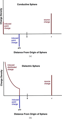
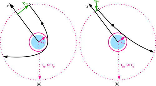
FIG. 2 Critical orbit, showing the boundary between capture and escape for ions with a given kinetic energy approaching a particle with (a) opposite charge and (b) similar charge. (Color figure available online.)

Before we apply this new potential, an accurate description of the particle and the ion is needed. For an aqueous particle, we can assume that the particle is a charged conductor that allows charge to redistribute itself across the surface. On the other hand, for a solid, dielectric particle, e.g., a dry polystyrene bead, we assume that the charge is in the center of the particle and immobile. When the ion approaches the particle, it will induce redistribution of the charge in the particle.

Depending on its properties, the ion involved in the above interaction may be described either as a collection of constituent molecules or as a large, single, continuous entity. A small ion or ionic cluster is well described as a charge embedded in an unpolarizable material. A better description of the near interaction between the ion and the particle in such a case would require detailed information about both the ion and the particle surface chemistry, and is well outside the scope of this article. On the other hand, a large ion cluster can be modeled as a charge fixed in the center of a dielectric sphere. In each case, the interaction cross-section is altered by the Coulomb interaction. For a particle whose kinetic energy is significantly greater than its potential energy, r_a ≈a_i +a_p . However, as the particle slows down, there are distinct limiting interaction radii for the attractive and repulsive cases. In the attractive case, the ion capture orbit can increase in size until it reaches a maximum at r_a =r ₀, where the ion's relevant life began. In the repulsive case, the force includes two components: the force between the source charges, and the force exerted by the induced images on the sources. If, as in Earth's atmosphere, the dielectric constant of the particle and/or ion is greater than that of the surrounding atmosphere, then the images induced on them will exert an attractive force that may exceed the repulsive force between the source charges. There exists a radius, r_f , where these two forces cancel. In order for the ion to be captured, it must have enough kinetic energy to reach r_a =r_f or r_a =a_i +a_p , whichever is greater. The ion's trajectory toward the particle surface is, therefore, curved toward/ away from the particle due to the attractive/repulsive forces between the two. This lensing effect will alter the capture cross-section presented to ions approaching the particle. The radius of this modified capture cross-section will be called b ₀, as illustrated in Figure 2. And, if r_a =r ₀, it's maximum value, then b ₀=r ₀ as well.

Lastly, we consider the effect of adding a third body, i.e., a neutral gas molecule, to the interaction between the ion and the particle. An ion with too much kinetic energy to be trapped by the Coulomb force described above may still strike a neutral gas molecule and lose sufficient energy to be trapped in the particle's potential well. Three-body trapping is only relevant in attractive interactions, where a smaller kinetic energy aids ion capture.

Now that we have introduced the relevant physical interactions in the system, we can proceed with the construction of a model.

MODELING FLUX COEFFICIENTS

We begin this process with a few physical parameters in hand that we will use to derive several other relevant parameters. We are given the ion mobilities at a set temperature and pressure, and the ion masses, as well as the gas characteristics and the ambient atmospheric conditions from HF. From this, we can derive the mean free paths of the ions and the gas, as well as the effective radius of each.

For ions, the base property is the ion mobility, μ _i , which will ultimately be used to calculate both the mean free path and effective radius. According to the kinetic theory of gases for hard sphere molecules, the ion mobility varies with temperature, T, and pressure, P, according to , where the subscript 0 denotes a reference state at which the mobility is known. Although, in air, ion mobilities cannot actually be determined using hard sphere relationships due to the polarizability of the gases, the scaling relationships for pressure and temperature should still hold true (Tammet 1995). Attractive and repulsive forces between the ions and the surrounding gas molecules can become important at low temperatures or high densities, when the potential energy begins to swamp the kinetic energy (Loeb 1939). The diffusivity is related to the mobility through the Einstein relation, . Here, is the Boltzmann constant, and e is the electric charge. The mean free path of the ion is consistent with HF (Hoppel and Frick 1986; Seinfeld and Pandis 1998). M _ion and M _gas are the masses of the ion and gas, respectively, and is the mean speed of the ion. For the gas molecules, the mean free path and effective radius can be estimated from the viscosity, η. The viscosity varies with T according to Sutherland's formula, , where the subscript 0 refers to a known viscosity reference state. Here, S_c is the so-called Sutherland's constant, which depends on gas composition. The mean free path of the gas molecules is, therefore, (Seinfeld and Pandis 1998). The effective radius of a gas molecule, , is calculated by equating two formulations for the mean free path, one based on gas viscosity, and the other on the interaction cross-section between the gas molecules. The effective radius of an ion in the gas,

is calculated in the same manner (Seinfeld and Pandis 1998).

With these relations in hand, the interactions between individual particles discussed in the background section can be used to determine the behavior of the ensemble. We have assumed that the only force acting upon the ion is exerted by a central ion/particle. This is a good approximation when the concentration of ions in the atmosphere is dilute. This is true at atmospheric temperatures for n ^1/3 _i ≪10⁴ ions/m³, where n_i is the total concentration of ions of charge i (Fuchs 1947; Natanson 1959). In this dilute limit, the force exerted by the atmospheric ions is negligible (Natanson 1959).

Following Natanson (1960) and Fuchs (1963), we consider transport in two regions: (1) an outer region where a continuum transport model is applied, and (2) an inner region that begins approximately one ion mean free path from the particle surface. Ion transport in this outer region is described by the convective diffusion equation,

where

describes the ion flux of species i to a particle of charge k. This flux includes both the Brownian diffusion and electrophoretic migration as a result of the Coulomb force between the ion and the particle. If (n_i ρ³)^1/2≪1 and qρ³≪1: ρ is the ion capture radius about the particle, and q is the volumetric ion creation rate, so that ion destruction and creation events are very rare (Fuchs 1947; Natanson 1959), then at ambient temperatures one can also assume that the diffusive flow is stationary,

Combining Equations (3), (4), and (5), we obtain

Integrating over the entire limiting sphere surface yields the ion current of species i to a particle of charge k in the continuum regime,

Integrating Equation (7) subject to the boundary condition that the ion concentration far from the particle surface is

which yields the steady-state current,

This ion current in the outer region, where this continuum model applies, must match that of the inner kinetic region,

at the radius of the limiting sphere, r ₀=a_i +a_p +Γλ _i . For the purposes of this model, we shall assume that Γ=1. The microscopic current within the limiting sphere is, in general, proportional to the ion density. (Henceforth, λ _i can be taken as Γλ _i in order to relax this assumption.) f(c ₀) is the probability that the ion will be captured by the particle; c ₀ is the ion speed at r ₀; and b ₀ is the modified cross-section radius. By setting the two currents equal at the limiting sphere, we can solve for n_i . In the dilute limit considered here, the ion current is proportional to the ion concentrations, so we define a flux coefficient as

Using Equations (9) and (10), this becomes

This flux coefficient depends on the molecular speed of the ion. We seek the average for all aerosol particles of a given size. Natanson (1960) found this by calculating the ensemble average in several limiting cases, but did not solve for the general form of ⟨β _k,i ⟩. Keefe et al. (1968) simplified this more general computation by calculating ⟨c ₀ b ² ₀(c ₀)⟩, and estimating ⟨β _k,i ⟩ by substituting this value for c ₀ b ² ₀(c ₀) in Equation (12). He compared these estimates with those obtained substituting different values of c ₀ into Equation (12) to identify a characteristic ion speed, c _char, for which this β(c _char) _k,i ≈⟨β _k,i ⟩ for a given particle/ion combination. HF use two of these characteristic speeds from Keefe in their calculations, one for ion–neutral particle interactions, and the other for ion–charged particle interactions.

The use of a characteristic value for c ₀ oversimplifies the estimation of ⟨β _k,i ⟩, as can readily be seen for repulsive interactions. Consider a Maxwellian distribution of ion speeds, which has a long tail on the high-speed end of the distribution. In spite of the repulsive interaction, some small fraction of the ions will always have sufficient kinetic energy to overcome the repulsive forces and reach the particle surface, a fact that is overlooked in the Keefe et al. (1968) and HF models. Keefe et al. (1968) also introduced a questionable renormalization to his estimate of ⟨c ₀ b ² ₀(c ₀)⟩ for repulsive interactions. Our analysis eliminates all of these unnecessary approximations. However, it still does not consider the effects of a strong potential on the ion speed and trajectory at the limiting sphere (Gopalakrishnan and Hogan 2012).

We follow Natanson and calculate,

using the normalized Maxwellian speed distribution, F(c ₀, T), without approximation to obtain the final form of the flux coefficient. However, to evaluate ⟨β _k,i ⟩, we must first find b ₀(c ₀) and f(c ₀).

We begin with the derivation of b ₀(c ₀) by examining the equation of motion of the ion for escape orbits. For any ion that escapes, energy and angular momentum are conserved, so the total energy of the system is

where c is the speed of the ion at any r<r ₀. c ² can be broken into its radial and tangential components, so

The tangential component can be written in terms of the ion's angular momentum, l, as

The radial velocity thus becomes

Applying the chain rule to yields

Thus,

The angular momentum, l=M _ion c ₀sin(θ)r, is conserved thr- oughout the ion's orbit, as there is no torque on the ion. Defining b(c ₀)≡rsin(θ), the angular momentum becomes l=M _ion c ₀ b(c ₀). If we choose a Cartesian coordinate system, CS1, with its origin at the center of the aerosol particle and the z-axis antiparallel to the initial trajectory of the ion, then b(c ₀) is a line segment perpendicular to the z-axis, connecting the axis to the ion at r ₀. The minimum b(c ₀) to describe an escape orbit is b ₀. Substituting l into Equation (18) yields

The minimum radius of the closest approach, r_a , where is called the apsoid. For a given apsoidal radius,

b ₀ must now be found. Only b ₀ for which

are physically attainable. The upper bound limits the solution to ions that approach the particle. The lower bound is set by the sum of the radii of the two bodies, where the ion would make physical contact.

This can be mathematically determined by finding the apsoidal radius, r_a , at which b ² is a minimum, i.e.,

subject to the constraint that

If this mathematical minimum leads to r_a >r ₀, we find b ₀=r ₀ and r_a =r ₀, since the capture cross-section radius cannot exceed that of the limiting sphere. If r_a <a_i +a_p , we find b ₀=0 and r_a =a_i +a_p . For a repulsive interaction wherein the ion has insufficient kinetic energy to achieve physical contact with the particle, the capture cross-section diminishes to 0. Since only deterministic two-body (ion + particle) interactions have been considered at this point, f(c ₀)=1. This constraint will be relaxed when random collisions of the ions with background gas molecules are taken into account in the discussion of so-called three-body trapping.

In the HF model, the boundary between the diffusive and the free molecular regime is defined by , so

A more general form of this equation allows the two radii at which the potential is evaluated to be varied to account for electrostatic lensing between the two points:

The HF limiting sphere radius, r_HF , can only be used if a constant characteristic value is assumed for the initial ion speed. In the present model, we consider the entire Maxwellian speed distribution. This includes low speeds for which r_a →∞ as the ion's kinetic energy goes to 0. This implies that r_HF →∞ as does the capture cross-section, b_HF . More problematically, this means that the capture cross-section, b_HF , is defined in terms of a different limiting sphere radius, r_HF , for each c. Instead, we begin our calculations at r ₀, where an ion begins with a speed c ₀ with probability F(c ₀, T).

THREE-BODY TRAPPING

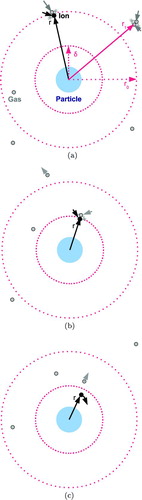
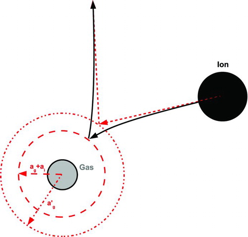
Presently, our limiting sphere model assumes that only two bodies, the ion and the particle, exist within that sphere. But the mean free path is just that, a mean distance between collisions. The ion still has a finite probability of collision within the limiting sphere. If it does collide, the ion's energy will be altered, possibly leading to capture. This mechanism dominates charge capture in dusty plasmas (Khrapac and Morfill 2009). This interaction, known as three-body trapping in the atmospheric literature, and as charge-exchange collision in the field of dusty plasmas, is illustrated in Figure 3. In the present model, the ion is considered captured if it has insufficient kinetic energy to escape the limiting sphere after collision with a neutral gas molecule. By approximating the background gas as a homogeneous, isotropic medium, the probability that an ion with a given trajectory will collide with a neutral gas molecule may be calculated using the Beer–Lambert law.

FIG. 3 Schematic of the steps involved in three-body capture. (a) The ion undergoes its last random scattering at radius r ₀. (b) The ion collides with a gas molecule at radius r⩽δ, losing kinetic energy. (c) The ion enters a collision course with the particle. (Color figure available online.)

To calculate the energy loss required for capture, we must consider the details of the ion–gas collision in the aerosol particle potential well. The ion begins a distance r ₀ away from the center of the particle, having just undergone its last random collision. Unless a collision occurs, the ion has kinetic energy

where φ is the potential between the ion and the particle, and ▵ is the potential between the ion and the gas molecule. The molecule begins a distance r ₁=a_g +a_p +λ _g away from the center of the particle and has kinetic energy,

where ψ is the potential between the molecule and the particle, and c _g0 and c_g are the gas molecule speed at r ₁ and r<r ₁, respectively. In order to develop a simple model that accurately characterizes the interaction between the three bodies, we would like to model the interaction between the ion and the molecule as the interaction between two 3D, perfectly elastic spheres, where Δ(r)=0. This is possible if the deflection of the trajectories by the attractive force is sufficiently short ranged. To describe how, we move into a frame of reference centered on the molecule,

Here,

where θ and θ′ are illustrated in Figure 4. Now, as illustrated in Figure 5, an attractive force between the two species will curve the ion's path toward the molecule. However, far from the molecule, the trajectory of the ion, both before and after collision, will reach an asymptote. This asymptotic trajectory can also be reached with two perfectly elastic spheres with no potential between them if the effective radius of the gas molecule is increased. We calculate this enhanced radius in the same manner as the impact parameter for an ion moving toward a particle,

FIG. 4 Conversion to primed frame.

FIG. 5 Collision between an ion and a gas molecule with an induced dipole moment that leads to an attractive potential. The ion trajectory is shown by the solid line. The equivalent collision trajectory with a larger gas molecule and no potential is shown by the dashed line. (Color figure available online.)

where the ion travels a mean free path to reach the gas molecule. In Earth's atmosphere, the vast majority of gas molecules have no permanent electric dipole moment, so

where m is the induced dipole moment for N₂ or O₂; Ω is the polarizability of the molecule; ε₀ is the permittivity of free space; and G is the field produced by the ion. This implies that the potential energy between the molecule and the ion is

where s is the radial distance between the ion and the molecule.

The positive and negative ions present depend on the composition and RH of the gas (Lee et al. 2005). To determine the extent to which the ion–molecule potential may influence these collisions, we note that the H₃O⁺ and OH⁻ are common ions in Earth's atmosphere, and apply the molecular radius of water, 0.2 nm, to make an upper bound estimate of the effect. This underestimates the ion size and overestimates its mobility since most atmospheric ions are clusters of water molecules around an ionized core. For the gas molecule, we assume a radius of 0.1 nm since this is a fair representation of N₂ or O₂. For a gas molecule that has the root-mean-square average speed before collision, and an ion that is initially at rest, the effective radius of the gas molecule is (a′ _g )≈1.8(a_g +a_i ), which is comparable to that of the molecules and ions, 0.1 nm, but two orders of magnitude below the length scale of λ _i , our escape distance. Thus, we model the ion/molecule collision as one between elastic spheres.

In these collisions, momentum can only be transferred in the direction of the normal force, and the normal force will not necessarily transfer all the momentum to the particle at rest. Conservation of momentum and the law of cosines lead to the expression

where p is the momentum of a species, and the subscripts i and g refer to the ion or the gas, while the f subscript refers to the state after collision, and its absence refers to the state immediately before collision. The prime superscript refers to the modified frame of reference. This interaction and the relevant angles, ϵ and ϵ′, are shown in Figure 6. Conservation of energy leads to

FIG. 6 The collision between an ion and a gas molecule of different size and mass. (Color figure available online.)

Combining Equations (32) and (33), we get, after some rearrangement,

which excludes the trivial case where (p′ _i )²=(p′ _if )²=0. HF, Natanson (1960), and Fuchs (1963) only considered head-on collisions, for which

Translating p′ _if into our original frame of reference and returning to the final speed yields

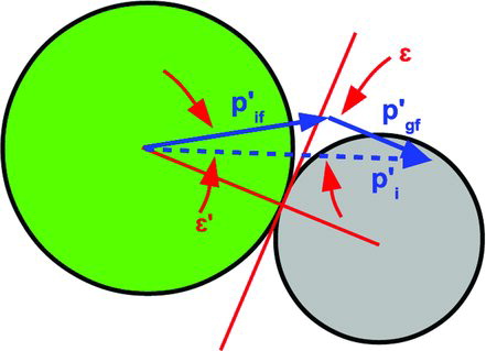
After applying Equation (34) and several trigonometric identities, we find

where

Equation (37) describes all possible collisions, and can be used to derive an ensemble average interaction between an ion and a gas molecule as a function of the ion's kinetic energy. The square of the ion velocity is averaged over all possible trajectories, 0<θ<2π, between the ion and the gas molecule to find

Substituting the molecular kinetic energy immediately before collision, Equation (26), and averaging over the Maxwellian distribution of gas molecule velocities yields

The ensemble average with respect to ϵ of A is calculated in the range and yields,

Substituting Equations (25) and (41) into Equation (39) yields

If the potential energy change for the gas molecule is small, , this simplifies to

The deviations produced by this assumption are small, <7%, even for a 1 nm singly charged particle, and <13% in the unlikely event (López-Yglesias and Flagan 2013) that the particle is doubly charged. For particles of radii 10 nm and larger, the deviation will be ∼0.1% or smaller for a well-modeled distribution.

Ion capture requires

The equality applies at the three-body trapping radius, r=δ; the resulting potential energy can now be used in Equation (20) to calculate the capture cross-section radius b _δ.

The above analysis is applicable for a gas that does not have permanent dipoles, and whose ion species do not consist of free electrons. In this case, the unimolecular force scales as r ⁻⁵. If, instead of having only induced dipoles, the gas has a permanent dipole moment, the force would act over a considerably longer range, r ⁻³.

Natanson (1960) applied a similar approach, but assumed that the ion and gas molecule both have kinetic energy 3k_BT/2 at r ₀, and the gas molecule experiences no potential. The HF model took a different approach. This energy for the difference of potentials is based on the empirically determined ion recombination distance, H, of Natanson (1959). This method substitutes

for the difference in potential energy in Equation (44). Here, W is the energy associated with two singly and oppositely charged point ions exerting a force on one another. This formulation omits the possibility of multiple charging, image charge, and finite size effects. We shall show later that the omitted interactions are important for the most populous species, the neutral particles, and will introduce a theoretical proportional relation to account for ion properties in the calculation of H.

To consider the influence of the Maxwellian distribution of initial ion speeds, f(c ₀), on the probability of ion capture, f(c ₀) consider the life of a single ion within the sphere. Because the gas molecule collision with an approaching ion is stochastic in nature, some ions that enter the three-body capture sphere will escape. We define a new Cartesian coordinate system, CS2, identical to CS1, defined above, with one exception: the z-axis is antiparallel to the trajectory of the ion at r=δ, rather than at r=r ₀ as in the case of our model of the two-body collision, or r_HF =δ+λ in the HF model. The angle between the ion trajectory at r=δ and the z-axis is named θ _c as shown in Figure 7b. To calculate the probability of an ion–molecule collision, we estimate the distance that the ion travels through the δ sphere as ∼2δcos(θ). By the Beer–Lambert law, the ion has a probability of exp(−2δcos(θ)/λ _i ) to pass through the sphere without a collision if θ is greater than the maximum angle, θ _c , that leads to direct intersection with the particle. The polar angle, θ, defines a ring about the z-axis across the surface of the sphere with radius δsin(θ). All ions of a given speed that travel parallel to the z-axis through the sphere at a given polar angle θ will suffer the same probability of collision. The probability that an ion will enter at any given angle between θ and θ+dθ is proportional to the infinitesimal ring cross-section at that θ perpendicular to the ion path divided by the total cross-sectional area of the δ sphere, or 2cos(θ)sin(θ)dθ. Integrating from θ _c to π/2 yields the total probability of the ion avoiding capture, once it enters the sphere, i.e.,

FIG. 7 Three-body capture and the calculation of the critical angles between definite and possible capture, θ _c , θ₁, and θ₂. (Color figure available online.)

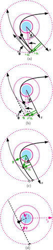
θ _c can be determined by expressing the exponential in the integrand for the probability as an infinite power series in δ/λ _i . The resulting expression

has one term with no dependence on , the unitless constant that characterizes probabilistic capture. This term is the fraction of captured ions that directly strike the aerosol particle. Simple trigonometry yields

where b_HF (r_a , δ) is the length of a line segment perpendicular to the z-axis, connecting the axis to the ion at δ as shown in Figure 7b. If the ion trajectory at δ is traced straight back to r_HF , as shown in Figure 7 c, then , where and . This geometry describes the three-body trapping as implemented in HF. The problem with this approach is that the b_HF (r_a , δ) term accounts for the electrostatic lensing only between the δ and r_a spheres, but does not extend the effect to the ion's initial position. HF only use b_HF (r_a , δ) and b_HF (δ, δ) to calculate f(c ₀). At the same time, HF use a different cross-section, b_HF (δ, δ+λ _i ), that accounts for lensing in the outer region of δ to δ+λ _i . However, the ion trajectory curvature makes the directly captured fraction of ions a function of where it is calculated, i.e., at r ₀ or δ.

As illustrated in Figure 7d, the present model accounts for the curvature of the ion trajectory along its entire path. The ratio of the modified, two-body cross-section, b ₀, to the modified, three-body cross-section, b _δ, as measured at r ₀, then becomes

This probability correctly accounts for the enhanced cross sections due to electrostatic lensing as previously suggested by Natanson (1960).

In any case, the three-body trapping need only be taken into account in a model when δ>r_a , as the ion will be caught regar- dless of whether it collides with a gas molecule when r_a >δ.

The three-body trapping described here is a first-order correction to the flux matching theory (Filippov 1993). Much could still be learned by using a full Monte Carlo simulation with molecular descriptions of the gas, ions, and particles.

MODELING THE CHARGE DISTRIBUTION

To deduce the statistical macroscopic charge state of an aerosol from the flux coefficients, one must solve a system of population balance equations for all sizes of particles that comprise the aerosol. This derivation is given in detail for particles of any size in López-Yglesias and Flagan (2013), so the results will only be briefly described here. Assuming a steady-state charge distribution, the ratio of the ion concentration at charge state k, N_k , and that at the next lowest charge state is

from which it follows that

may be used to obtain the ratio between the concentration of particles in charge state k and those with charge state 0. Summing over all charge states, one finds

In practice, the calculations are performed only over a finite range of charge states, −k⩽j⩽y. The charge distribution thus becomes

The validity of the steady-state assumption under different charging times and aerosol loadings is examined in detail in López-Yglesias and Flagan (2013).

Although the present work treats the negative and positive ions in this model as two singular species, this is a simplification. In reality, the ion masses and mobility follow a distribution, which depends upon the composition of the environment, and which will affect the resultant charge distribution (Lee et al. 2005).

TABLE 1 Initial parameters

Symbol	Value
T	298.15 K
P	101325 Pa
μ+ion	1.2 × 10^−4 m^2V^−1s^−1
μ−ion	1.35 × 10^−4 m^2V^−1s^−1
M +ion	150 Da
M −ion	90 Da
M gas	28.97 Da
η	18.27 × 10^−6 Pa s

RESULTS

Hoppel and Frick (1986) previously modeled the charging of conductive particles up to 500 nm in radius. The present model relaxes several approximations in the earlier work, and treats particles of any dielectric constant. Furthermore, the particle charge is allowed to induce an image in the ion cluster. To allow direct examination of the influence of the relaxed approximations and broader range of aerosol materials, we employ the same ion properties, shown in Table 1, while examining a range of dielectric constants.

Figure 8 shows the variation in the calculated flux coefficients as a function of particle size for a wide range of charge states. The predictions for conductive particles (solid lines) can be directly compared with those of HF (dotted lines). The two models agree well for large particles, though there are subtle differences that arise from consideration of the entire velocity distribution, and from the revised three-body trapping model, which is applied to all attractive interactions.

FIG. 8 Flux coefficients for negative (a), and positive (b), ions to aerosol particles of various charge states. (Color figure available online.)

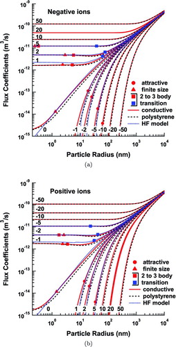
The induced-charge effect diminishes with decreasing size, causing the interactions to switch from attractive to repulsive at the sizes indicated by circles in Figure 8. These points correspond to the particle size at which there exists a cutoff speed below which the ion cannot reach the particle. Below this transition point, the present model diverges from that of HF, since, rather than averaging over the speed distribution, HF use a single equivalent speed. This leads to rapid decrease and sharp cutoff in their flux coefficients because the single speed used is no longer able to overcome the repulsive force. This difference becomes extremely important for calculating multiple charging events in a unipolar environment.

Another important difference between the two models is the consideration of finite ion size. HF assume that the ions are 0D points, which implies that their flux coefficients can decrease to zero with decreasing particle size. We may estimate the particle size below which finite ion size affects the flux coefficients as that for which the capture radius is the sum of both bodies’ radii when the ion is traveling at speed , where σ is the standard deviation of the Maxwellian distribution of ion speeds. Above the transition, the models agree well. Below this transition point, the present model approaches its asymptote, while the HF estimation continues to zero.

The situation is more complex for flux coefficients of oppositely charged ions and particles. Although there are transitions below which the appearance of the model changes, there is no smoking gun. The effects discussed in the beginning of this section are no longer subtle at low particle charge. The closest we can come to a true transition point may be when three-body trapping replaces two-body trapping in the HF model, shown as open or blue squares in Figure 8. Here, the difference between the two- and three-body models considered becomes very pronounced. The two- to three-body transition point for our model is denoted by a closed, or red, square in Figure 8. We may estimate this point by searching for the largest particle size where the resultant, unaveraged flux coefficient is larger in three-body trapping than in two-body trapping, while the ion is traveling at speed . Below the transition point of the HF model, their calculated flux coefficients are greater than those of the present model due to the revised energy calculation and geometric effects discussed in Section Three-Body Trapping of this article. The two models would differ even more wildly at the smallest particle sizes if not for the fact that our model also undergoes a finite size transition, increasing our flux coefficients at these low sizes.

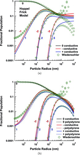
FIG. 9 Steady-state charge distributions for the HF model (a), and the present model (b). (Color figure available online.)

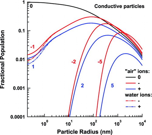
In addition to reexamining flux coefficients for conductive particles, we have also explored the difference in flux coefficients due to a lower dielectric constant. In particular, we examine aerosol particles with a dielectric constant of 2.6, corresponding to polystyrene, which is often used for calibrating DMAs. As expected, the image force for dielectric particles is weaker than for conductive ones, markedly accelerating the decrease of the flux coefficient in like-charged and ion-to-neutral-particle interactions. Ion-to-neutral-particle interactions regain the same flux coefficients as the conductive aerosol at small particle size due to the finite size transition. Oppositely charged particles are only affected in the transition between the dominance of the image charge force and source charge force.

Figure 9 shows the steady-state fractional population of the aerosol as calculated from the flux coefficients above. The corrections to HF at the high end of the model have previously been discussed in López-Yglesias and Flagan (2013). In the present model, the charged fraction approaches an asymptote at small sizes. The curvature results from the finite size effect in the ion-to-neutral-particle flux coefficients. For doubly charged particles of opposite polarity, HF predict that the charging probabilities for positive and negative particles cross as size decreases, albeit at a very low charging probability. This crossing is eliminated in the present model by considering the full Maxwellian speed distribution. The Wiedensohler (1988) approximation is also included for the sake of comparison. Its parameters are based on the earlier works of Hussin et al. (1983), Wiedensohler et al. (1986), and HF. It is an approximation of the HF model valid for particles of 0.5⩽a_p ⩽500 nm radii that are neutral or have ±1e of charge, and for particles of 10⩽a_p ⩽500 nm radii that have ±2e of charge. For higher charge states, Wiedensohler applied the analytical solution from Gunn and Woessner (1956), which is only valid for particles with a_p >25 nm because it is based upon an equilibrium Boltzmann distribution. Furthermore, as clearly discussed by Fuchs (1963) and Mayya (1994), the equilibrium model is not applicable to ambient temperature aerosol charging because the “reverse reaction” to charge attachment, charged species desorption, is energetically unfavorable. Nonetheless, within the working regime of Gunn's model, our model agrees well. However, it deviates significantly from the HF charge distribution above 400 nm in radius and below 3 nm for particles with ±1e or ±2e of charge.

FIG. 10 Flux coefficients for negative (a), and positive (b), ions to aerosol particles of various charge states at P = 4480 Pa and T = 218.15 K, conditions at an altitude of ∼20 km. (Color figure available online.)

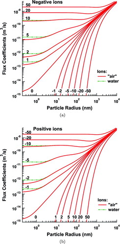
FIG. 11 The resultant steady-state charge distribution using the present model at an altitude of ∼20 km. (Color figure available online.)

We also explored the effects of the image charge induced on the ion by the particle, for a water cluster with a dielectric constant of 80.1. The inclusion of the ion image charge raised the value of the flux coefficients for oppositely charged particles and ions by a maximum of 10% for singly charged particles below 2 nm in radius, leading to a similar decrease in the fraction of charged particles in the steady-state distribution in this size range. Above this size and/or particle charge, the effects are <1% for oppositely charged species. The flux coefficients of similarly charged particles and ions increase by up to seven orders of magnitude in the nanometer size regime, but the ratio of these flux coefficients to those for the ion-to-neutral interactions, the dominant source of charged particles in this size regime, is still insignificant to the steady-state charge distribution.

Previous studies of aerosol charging only consider normal laboratory conditions, but aerosol measurements are made in many other environments. In particular, DMAs are extensively used to measure size distributions from airborne platforms. Therefore, we also consider the effect of a change in pressure and temperature, P = 4480 Pa and T = 218.15 K. This simulates the atmospheric conditions at an altitude of 20 km, as an upper bound to present DMA measurements. For this substudy, we consider only the conductive particles. The results are shown in Figures 10 and 11. The flux coefficients between doubly and, especially, singly charged particles and ions of opposite charge are significantly reduced from the coefficients at sea level. Moreover, the flux coefficients for attractive interactions at high charge levels exhibit a pronounced minimum in the transition between the fine particle asymptote and the continuum diffusive regime. These effects are due to the greatly increased mobility and mean free path at high altitudes. The ions now begin their relevant life spans further away, reducing the effect of the attractive force, especially at small particle charge. Because of this, the effects of image charge on a water ion as opposed to an “air” ion are significantly more pronounced than at ground level, leading to deviations of a factor of ∼2 in both the flux coefficients and the steady-state charge distribution for small particle sizes. These reduced flux coefficients lead to a significant increase in the singly charged fraction of the aerosol population at nanometer size. Thus, the use of sea-level charging probabilities to invert airborne DMA measurements may lead to significant errors in the estimated particle size distribution depending on the altitude.

CONCLUSIONS

We investigated several corrections and extensions to the aerosol charging model of Hoppel and Frick (1986). The description of the potential between an ion and an aerosol particle was broadened to include dielectric bodies, and to allow for image charges to be induced on the ion. The effective radius of the ion, a_i , was derived, and a fixed starting point for the trajectory of the ion in its interactions with an aerosol particle, based solely on a_p , a_i , and λ _i , r ₀, was formulated for use. The resulting flux coefficients were then averaged over the Maxwellian velocity distribution of the ion at ambient conditions to obtain the ensemble average. The mechanism for three-body trapping was also revisited and improved upon. The calculation of the average energy lost in an ion–gas molecule collision within a particle's potential well was re-derived from kinetic theory, and the probability of ion capture was also revised to account more fully for the curvature of the ion's flight. In light of these changes, the flux coefficients and steady-state distributions of our model were compared with those from HF and the Wiedensohler approximation.

Using the same ionic and ambient parameters as HF, we found several points where the present model diverged significantly from the flux coefficients in HF. Consideration of the Maxwell–Boltzmann distribution of ion speeds leads to significant deviations from the HF ion flux coefficients for like-charged aerosol–ion interaction at 40 nm radii particle and below. Transitions for oppositely charged aerosol–ion interactions occur at radii <85 nm due to a combination of three-body trapping and the ion's finite size. Ion-to-neutral-particle interactions begin to deviate at low nanometer sizes due entirely to finite-size effects. These changes in the flux coefficients are reflected in quantitative and qualitative changes in the steady-state charge distribution. The most significant of these changes is a leveling off of the singly charged aerosol population at small radii due to finite size effects.

Varying parameters within the new model leads to further deviations from the original theory. Dielectric particles, often used to calibrate DMAs, have a significantly reduced image charge. This manifests itself as a reduced population of charged particles at all particle sizes due primarily to the suppression of the flux coefficients for like-charged particles and ions, and the reduced probability of ion capture by neutral particles. The latter effect reduces to ballistic ion capture in the absence of image charge. The population of singly charged aerosol particles can decrease by .

We also examined the effect of atmospheric conditions on particle charging. At altitudes near the tropopause, the pressure and temperature both drop, increasing the ion mobility and mean free path, and decreasing the gas viscosity. This suppresses ion–particle recombination at small particle charge, increasing the fraction of charged aerosol at nanometric size by a factor of ∼3 compared with sea-level conditions.

Finally, for the bipolar charging that was the focus of this article, the image charge on the ion has a small effect, at most 10%, on the steady-state aerosol charge distribution at ground level, but causes deviations of up to a factor of 2 at high altitudes for nanometer-sized particles. This ion image-charge potential may also be important in long-time exposure to a unipolar environment, particularly in the nanometer size range.

The corrections and additions included in this study cause a wide range of changes to the aerosol charge distribution, especially for nanometer particles. As DMA studies continue to push the lower limit of observed particles into this range, we feel that the effects presented here may prove useful for enhancing the accuracy of data in this size regime. The previously reported deviations at large particle size also lead to substantial overestimates of the particle concentrations above about 200 nm radius. This may significantly bias DMA-based estimates of the mass concentration of fine particles. We have provided curve-fits to the flux coefficients and charging probabilities in the manner of Wiedensohler, but note that these fits, and all of the calculations on which they are based, employ the ion properties that were used in the earlier Hoppel and Frick (1986) model. The ion properties, and this dependence on atmospheric parameters, especially RH, need to be reexamined, but this is beyond the scope of the present work.

NOMENCLATURE

a p/i/g	=	radius of particle/ion/gas
a′ g	=	enhanced radius of interaction between an ion and gas molecule
A	=	, a dimensionless parameter in three-body trapping
b	=	modified interaction cross-section radius
bHF	=	modified interaction cross-section radius for three-body trapping in Hoppel–Frick
b 0	=	square root of the minimum physical b 2(c 0)
b δ	=	b 0 for three-body trapping
Bi	=	numerical fit coefficient
c	=	speed of ion at r<r 0
c 0	=	speed of ion at r 0
	=	mean speed of ion
cc	=	cutoff speed in repulsive interactions
c char	=	characteristic speed of ion in the Keefe et al. (1968) approximation
cf	=	speed of ion after collision with gas molecule
cg	=	speed of ion at r<r 1
c g0	=	speed of gas molecule at r 1
c′	=	speed of ion in reference frame with gas molecule at rest
c′ g	=	speed of gas molecule in reference frame where gas molecule is at rest
D ion	=	diffusivity of ion
e	=	elementary charge
E	=	energy in the ion–particle system
f	=	probability of ion capture
F	=	normalized Maxwell distribution
g(k)	=	numerical approximation function
G	=	electric field produced by ion
h	=	maximum charge state, negative
H	=	ion–ion trapping distance
i	=	ion charge
I k,i	=	ion current of charge i to particle of charge k
j	=	index of charge states
J k,i	=	flux of ion with charge i to particle of charge k
k	=	number of charges on particle
kB	=	Boltzmann constant
l	=	angular momentum
m	=	induced dipole moment
M ion/gas	=	mass of ion/gas molecule
n	=	concentration of ions
Nk	=	concentration of particles in charge state k
NT	=	total aerosol concentration
p i/if/g/gf	=	momentum/final momentum of ion/gas
p′ i/if/g/gf	=	momentum/final momentum of ion/gas in frame c′ g =0
P	=	pressure
P 0	=	initial pressure
q	=	ion creation rate per unit volume
r	=	distance from ion to aerosol particle
ra	=	radius of smallest escape orbit apsoid
rf	=	radius where force on ion is zero in repulsive interactions
rHF	=	λ i +ra or λ i +δ, whichever is greater, r 0 as used by Hoppel and Frick (1986)
r 0/1	=	radius where ion/gas molecule begins its relevant life span
s	=	distance between ion and neutral gas molecule
Sc	=	Sutherland's constant
t	=	time
T	=	temperature
T 0	=	initial temperature
W	=	Hoppel–Frick change in potential for three-body trapping
x	=	distance from center of ion/particle to portion of distributed image charge
y	=	maximum charge state, positive
α	=	ion recombination coefficient
β k,i	=	flux coefficient of an ion of charge i to a particle of charge k
γ i/p	=	, a dimensionless parameter for calculating image charge
Γ	=	dimensionless factor of order unity
δ	=	three-body trapping radius
δ	=	potential energy between ion and gas molecule
ϵ	=	angle between p′ gf and particle's radial vector
ε0	=	permittivity of free space
η	=	viscosity of gas
θ	=	three-body trapping angle
θ c	=	critical angle demarcation between two- and three-body trapping
λ i/g	=	mean free path of ion/gas
μ i	=	ion mobility
Ξ i0/g0/i1/g1	=	kinetic energy of an ion/gas molecule at r 0/just before collision
ξ p/i	=	, a dimensionless parameter for calculating image charge
ρ	=	ra or δ, whichever is greater
υ p/i	=	, a dimensionless parameter for calculating image charge
φ k,i	=	potential energy between an ion of charge i and a particle of charge k
χ i/p/0	=	dielectric constant of ion/particle/atmosphere
ψ	=	potential energy between gas molecule and particle
Ω	=	polarizability

Acknowledgments

The authors thank Lindsay Yee for her time spent editing and discussing this manuscript. They would also like to thank an anonymous reviewer for doing an outstanding job; the reviewer raised interesting scientific points that go well beyond the scope of the current work. Finally, the authors thank the NASA Astrobiology Institute through the NAI Titan team managed at JPL under NASA Contract NAS7-03001 for the funding of this project, and the Ayrshire Foundation for their support in making computing resources available.

APPENDIX: EMPIRICAL FITS

Flux coefficients and the steady-state charge distribution were calculated for particle sizes between a_p =0.2  nm and a_p =10  μm. The approximate formula used for either is in the style of Wiedensohler (1988). B_i (k) are fit coefficients determined by a least square regression analysis. The fit coefficients for each case covered in the article are given in the tables in the online supplemental information up to ±2e particle charge along with the relative error. Delimited tables are available in the individual text files corresponding to the tables in the online supplemental information section with the B_i necessary to calculate both the flux coefficients of particles with charge up to ±10e (±2e for water ions) and the steady-state charge distribution for particles with charge up to ±5e (±2e for water ions).

To calculate the steady-state fractional population of particles with charge >|5e|, the expression from Gunn and Woessner (1956) may be used,

REFERENCES

- Amadon , A. S. and Marlowe , W. H. 1991a . Cluster-Collision Frequency. I. The Long-Range Intercluster Potential . Phys. Rev. A , 43 : 5483 – 5492 .
- Amadon , A. S. and Marlowe , W. H. 1991b . Cluster-Collision Frequency. II. Estimation of the Collision Rate . Phys. Rev. A , 43 : 5493 – 5499 .
- Filippov , A. V. 1993 . Charging of Aerosol in the Transition Regime . J. Aerosol Sci. , 24 ( 4 ) : 423 – 436 .
- Fuchs , N. A. 1947 . On the Magnitude of Electrical Charges Carried by the Particles of Atmospheric Aerocolloids . Izvestiya Acad. Sci. USSR Ser. Geogr. Geophys. , 1l : 341 – 348 . In Russian with English summary
- Fuchs , N. A. 1963 . On the Stationary Charge Distribution on Aerosol Particles in a Bipolar Ionic Environment . Geofis. Pura Appl. , 56 : 185 – 192 .
- Gopalakrishnan , R. and Hogan , C. J. 2012 . Coulomb-Influenced Collisions in Aerosols and Dusty Plasmas . Phys. Rev. E , 85 : 026410
- Gunn , R. and Woessner , R. H. 1956 . Measurements of the Systematic Electrification of Aerosols . J. Colloid. Sci. , 11 : 254 – 259 .
- Hoppel , W. A. and Frick , G. M. 1986 . Ion-Aerosol Attachment Coefficients and the Steady-State Charge Distribution on Aerosols in a Bipolar Ion Environment . Aerosol Sci. Technol. , 5 : 1 – 21 .
- Hussin , A. , Scheibel , H. , Becker , K. and Porstendorfer , J. 1983 . Bipolar Diffusion Charging of Aerosol Particles-1. Experimental Results Within the Diameter Range 4–30 nm . J. Aerosol Sci. , 14 : 671 – 677 .
- Keefe , D. , Nolan , P. J. and Scott , J. A. 1968 . Influence of Coulomb and Image Forces in Combination of Aerosol . Proc. R. Irish. Acad. , 60A : 27 – 44 .
- Kirkby , J. , Curtiu , J. , Almeida , J. , Dunne , E. , Duplissy , J. and Ehrhart , S. 2011 . Role of Sulphuric Acid, Ammonia and Galactic Cosmic Rays in Atmospheric Aerosol Nucleation . Nature , 476 : 429 – 433 .
- Khrapac , S. and Morfill , G. 2009 . Basic Processes in Complex (Dusty) Plasmas: Charging, Interactions, and Ion Drag Force . Contrib. Plasma Phys. , 49 ( 3 ) : 148 – 168 .
- Lee , H. M. , Kim , C. S. , Shimada , M. and Okuyama , K. 2005 . Effects of Mobility Changes and Distribution of Bipolar Ions on Aerosol Nanoparticle Diffusion Charging . J. Chem. Eng. Japan , 38 : 486 – 496 .
- Loeb , L. 1939 . Fundamental Processes of Electrical Discharge in Gases , 112 – 120 . New York : Wiley .
- López-Yglesias , X. and Flagan , R. 2013 . Population Balances of Micron-Sized Aerosols in a Bipolar Ion Environment . Aerosol Sci. Technol. , 47 ( 6 ) : 681 – 687 .
- Lushnikov , A. A. and Kulmala , M. 2004 . Charging of Aerosol Particles in the Near Free-Molecule Regime . Eur. Phys. J. D. , 29 : 345 – 355 .
- Mayya , Y. S. 1994 . On the “Boltzmann Law” in Bipolar Charging . J. Aerosol Sci. , 25 : 617 – 621 .
- Nadykto , A. and Yu , F. 2003 . Uptake of Neutral Polar Vapor Molecules by Charged Clusters/Particles: Enhancement Due to Dipole-Charge Interaction . J. Geophys. Research , 108 ( D23 ) : 4717
- Natanson , G. L. 1959 . The Theory of Volume Recombination of Ions . Soviet Physics Technical Physics , 4 : 1263 – 1269 .
- Natanson , G. L. 1960 . On the Theory of Charging of a Microscopic Aerosol Particles as a Result of the Capture of Gas Ions . Soviet Physics Technical Physics , 5 : 538 – 551 .
- Neumann , C. 1883 . Hydrodynamischie Untersuchen nebst einem Anhang uber die Probleme der Elecktrostatik und der magnetischen Induktion , 279 – 282 . Leipzig : Teubner .
- Norris , W. T. 1995 . Charge Images in a Dielectric Sphere . IEE Proc.-Sci. Meas. Technol. , 142 ( 2 ) : 142 – 150 .
- Premnath , V. , Oberreit , D. and Hogan , C. J. Jr . 2011 . Aerosol Sci. Technol. , 45 : 712 – 726 .
- Seinfeld , J. and Pandis , S. 1998 . Atmospheric Chemistry and Physics , 454 – 459 . New York : Wiley .
- Tammet , H. 1995 . Size and Mobility of Nanometer Particles, Clusters and Ions . J. of Aerosol Sci. , 26 ( 3 ) : 459 – 475 .
- Tammet , H. and Kulmala , M. 2005 . Simulation Tool for Atmospheric Aerosol Nucleation Bursts . J. Aerosol Sci. , 36 : 173 – 196 .
- Wiedensohler , A. , Liitkemeier , E. , Feldpausch , M. and Helsper , C. 1986 . Investigation of the Bipolar Charge Distribution at Various Gas Conditions . J. Aerosol Sci. , 17 : 413 – 416 .
- Wiedensohler , A. 1988 . An Approximation of the Bipolar Charge Distribution for Particles in the Submicron Size Range . J. Aerosol Sci. , 19 : 387 – 389 .
- Yu , F. and Turco , R. 1998 . The Formation and Evolution of Aerosols in Stratospheric Aircraft Plumes: Numerical Simulations and Comparisons with Observations . J. Geophys. Research , 103 ( D20 ) : 25,915 – 25,934 .