The Effects of Unresolved Scalar Fluctuations During Homogeneous Nucleation

Abstract

The effects of the subgrid-scale (SGS) scalar interactions on nanoparticle nucleation are investigated via a priori analysis of direct numerical simulation data. The formation of dibutyl-phthalate (DBP) particles via homogeneous nucleation is simulated in a planar wake. Classical nucleation theory is used to model particle nucleation and the Navier-Stokes equations are coupled with the scalar transport equations to provide the fluid, thermal, and chemical fields. The data shows that particle nucleation is initially confined to the thin interfacial region or shear layers, where molecular diffusion is dominant. As the flow becomes turbulent nucleation increases significantly and the rate of particle formation increases by several orders of magnitude. To assess the effect of SGS scalar interactions on DBP particle nucleation, the temperature and mass-fractions are filtered and the resulting quantities are used to compute the nucleating particle field. Two filter widths are used to obtain varying levels of SGS interactions. Particle size distributions are computed to examine the particle fields produced. This work shows that the SGS interactions’ effect on nucleation has two distinct trends. In the proximal region of the wake, the unresolved interactions act to decrease particle formation. However, as the flow transitions or becomes turbulent the effect of the SGS interactions act to increase particle formation.

Copyright 2013 American Association for Aerosol Research

1. INTRODUCTION

Nucleation is understood to play a prominent role in such physical processes as condensation and evaporation, crystallization and the deposition of thin films, and its theoretical underpinnings were described as early as the late nineteenth century in Gibbs’ theoretical thermodynamic works. While nucleation mechanisms have been given considerable attention in past studies, there are still aspects of the processes, including the effects of fluid turbulence, that are not yet completely understood (Frenklach 2002; Bodenschatz et al. 2010). A better understanding of the interactions between the fluid dynamics and the nucleation physics is the key to understanding particle nucleation and improved modeling of vapor-phase particle formation and growth in complex flows (Jaenisch et al. 1998; Nilsson et al. 2001; Aristizabal et al. 2006).

A number of experiments have been carried out that study the formation of nanoparticles via nucleation. Lesniewski and Friedlander investigated the nucleation and subsequent growth of dibutyl-phthalate (DBP) particles in a free turbulent jet (Lesniewski and Friendlander 1998). Particle size distributions measured as a function of spatial location and scaling laws were developed that related final aerosol concentrations to initial flow velocity. Hämeri and Kulmala also studied the homogeneous nucleation of DBP, though in laminar flow diffusion cloud chambers (Hämeri and Kulmala 1996). While some work has indeed explored DBP nucleation under turbulent conditions (Anisimov and Cherevko 1985; Okuyama et al. 1987; Warren et al. 1987; Pyykönen et al. 2007; Fager et al. 2012), the majority of research has been confined to laminar flow systems, leaving the effects of fluid turbulence and small-scale interactions to speculation. Simple calculations were first used to explore the effects of turbulence on homogeneous nucleation and to relate the location at which nucleation is most prevalent to flow characteristics. Lesniewski and Friedlander (1995) looked into the effects of turbulence on nucleation by carrying out calculations for a jet in which the Lewis number was unity (thermal and mass diffusivities are equal) (Lesniewski and Friedlander 1995). They posited that turbulent fluctuations broadened nucleation across the shear layer as a result of pockets of unmixed, relatively hot, fluid being injected into cooler fluid. Additionally, they concluded that while turbulence greatly affected the distribution of the product particles, it had a lesser significant effect on the rate at which these particles were formed. The assumption that nucleation occurs exclusively in the shear layer contradicts the work of Clement (1985), which postulates that the Lewis number of unity assumption is inadequate for aerosol formation. And more recently, it has been shown that the effects of turbulent fluctuations on nanoparticle growth in turbulent shear flows are indeed significant (Das and Garrick 2010; Garrick 2011).

Our intent is to elucidate the effects of small-scale or unresolved interactions on particle nucleation. To accomplish this we perform direct numerical simulation (DNS) of DBP nucleation in a turbulent wake. We then use the DNS data to perform an a priori analysis on the effect that the unresolved scalars—temperature and DBP mass-fraction—have on the nucleation rate. As the scope of this work is limited to the modeling and simulation of nucleation, only the scalars themselves are filtered and analyzed. This is in contrast to more complicated physical quantities often analyzed in experiment or theoretical studies on how fluctuations affect nucleation Easter and Peters (1994). We utilize a spatial filter of varying width to separate the quantities into their means and fluctuations, compare the nucleation rate based on the exact and mean quantities, and evaluate unresolved scale quantities in a statistical manner. From this analysis, the effects of small-scale interactions (inherent in turbulent flow) on the nucleation are readily apparent.

2. FORMULATION

2.1. Fluid Transport

The flow under consideration is governed by the compressible Navier–Stokes equations in which the fundamental transport variables are the velocities u_i(x_i, t) in the x_i direction, pressure p(x_i, t) and the total enthalpy h(x_i, t). The conservation equations for the aforementioned variables are (1) (2) and (3) where τ_ij is the viscous stress tensor for a Newtonian fluid, k is the thermal conductivity, and C_p is the specific heat. The system is closed using the ideal gas equation of state, p = ρRT, where R is the gas constant and T is the temperature, obtained via dh = C_pdT.

2.2. Species Transport

The flow consists of two gases, a condensible vapor and a non-condensible carrier, or background gas. The mass-fraction transport equation is given by (4) where Y_i is the mass fraction of species i, is the diffusion coefficient and is the species sink due to particle nucleation. This term accounts for the conversion of the vapor to particles and will be zero for the carrier gas.

2.3. Particle Nucleation

One of the more commonly used approaches to nucleation modeling is classical nucleation theory (CNT). Given the pressure, temperature, species concentration, and material properties, CNT predicts a particular particle formation rate [particles/ (m³·s)]. The use of CNT is attractive as its mathematical simplicity renders itself amenable to use in large-scale simulations and has had success predicting nucleation rates observed in experiment (Friedlander 2000). Using CNT, and the correction factor of Girshick and Chiu (1990), the rate of particle formation is given by (5) Here, ρ_c is the condensed-phase density of DBP, σ is the surface tension, m_m is the species molecular mass, v_m is the volume of a molecule, k_B is the Boltzmann constant, and d_c is the critical diameter or the diameter of the nucleating particle according to the Kelvin relationship (Friedlander 2000), given by (6) where S is the saturation ratio, defined as the ratio of the vapor partial pressure of species i to the equilibrium (or saturation) vapor pressure at a given temperature, and given by (7) where p_mix is the local, thermodynamic mixture pressure, MW_mix is the mixture molecular weight and x_sat is the saturation mole fraction for species i. The factor c_nuc is a material-specific, empirical correction. Such factors are used to account for both inaccurate material properties and insufficient nucleation models and are applied to nucleation rate expressions to match observed rates for a given species (Pyykönen and Jokiniemi 2000; Harstad and Bellan 2004). The rate of aerosol mass being produced is obtained by multiplying the nucleation rate J_kin [particles/(m³·s)] by the mass of a nucleating droplet (kg), (8)

3. RESULTS

3.1. Flow Configuration

The flow of interest is a three-dimensional planar wake. The plane wake is comprised of gas issuing through nozzle, or slot, of height D at a velocity of U_o and temperature T_o into a co-flowing stream with velocity U_∞ and temperature T_∞. The velocity ratio is U_o/U_∞ = 0.25, and the Reynolds number, based on the velocity difference ΔU = U_∞−U_o is Re = ρ_oΔUD/μ_o = 4000. The gas is comprised of a mixture of dibutyl-phthalate (DBP) and nitrogen. The mass fraction of the condensible vapor DBP is Y_DBP = 7.09×10⁻³, which is chosen to achieve a saturation ratio at the inflow plane of S_o = 1. The temperatures are T_o = 400K and T_∞ = 300K. The Lewis number is , evaluated at the reference conditions, namely T_o. Lewis numbers—greater than unity—indicate that thermal diffusion is greater than species diffusion.

3.2. Physical Assumptions

Nucleation is an unsteady, non-equilibrium, process. Homogeneous nucleation theory suggests that molecular clusters grow in size due to the attachment of single molecules. These small molecular clusters are unstable until they overcome an energy barrier. The clusters that are stable nucleate at the critical diameter, d_c. This stability includes the balance of the kinetic energy of the constituent molecules, surface energy of the cluster, and other forces, including chemical and inter-molecular forces (Friedlander 2000). The time needed for this “nucleation process” is finite and may interact the with the time-scales of the flow (Wegener and Sreenivasan 1981). We have performed temporal simulations that compute molecular-cluster growth using the collision-based method following the work of McMurry (1983, 1980). The results of these simulations show that particles of the size produced in this work (less than approximately 3 nm) form stable clusters within 10⁻⁹s. The convective time scale in this work, based upon the Kolmogorov length scale, is much larger, approximately 10⁻⁴s. These results suggest that the nucleation time-scale is sufficiently fast such that the flow can be considered to be “frozen” while nucleation occurs. A recent work utilized this frozen eddy assumption (Di Veroli and Rigopoulos 2011). The heat release is taken into account by calculating the enthalpy based upon the DBP vapor mass fraction as nucleation converts vapor into particulate mass. This does not, however, take into account the heat released during the nucleation process. This approach alters the temperature field based upon the change in mass-fraction, which in turn affects the calculated nucleation rate. Though this heat release is accounted for, it is not significant under these flow conditions as relatively little vapor mass is converted to particles via nucleation.

The assumptions inherent in CNT and the kinetic model of Girshick and Chiu (1990) are acknowledged and subsequently adopted in this work. Specifically, these involve the nature of cluster formation at the molecular level. It is assumed that the molecular clusters that create nuclei are homogeneous, spherical, contain no charge, and retain the same properties of the bulk material (Girshick and Chiu 1990). The bulk properties of DBP are used here in accordance with CNT. This includes the density of DBP and the surface tension. We adopt the expression given by Nguyen et al. (1987) for the surface tension, σ = 0.0353−0.0000863(T−273.26) and saturation mole fraction, x_sat = exp(21.497−11497/T). Of note, the expression utilized for the saturation mole fraction leads to the appearance of an exponential term in the denominator of Equation (7(7) ). The use of a bulk value for the surface tension at the nanoscale becomes suspect (Friedlander 2000). Indeed, utilization of a size-dependent surface tension has been shown to affect nucleation rates for certain chemical species, though these expressions involve assumptions of their own (Onischuk et al. 2006; Liu and Garrick 2010). Additionally, while evaporation or “denucleation” can often be significant (Goodrich 1964), it is not considered here. Finally, the use of CNT often involves an empirical correction factor. In this work the value is taken to be c_nuc = 3.2×10⁻⁴, specific to DBP (Pyykönen and Jokiniemi 2000).

3.3. Numerical Specifications and Parameters

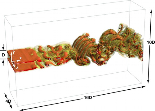
The transport equations are integrated using a hybrid MacCormack-based finite-difference scheme, which is second order accurate in time and fourth order accurate in space (Carpenter 1990; Kennedy and Carpenter 1994). A domain size of 16D×10D×4D is covered by a grid consisting of 1152×704×288 points in the x, y, and z directions. A schematic is shown in Figure 1. As this DNS simulation is used as a baseline in this work, the length scale of the smallest turbulent motion (Kolmogorov microscale) must be resolved. Here, an approximate of the Kolmogorov length scale η = Re^−1/4D is used (Tennekes and Lumley 1972). Using the parameters of this flow, the Kolmogorov length scale is approximately one order of magnitude larger than the grid spacing, which shows that the DNS resolution used is sufficient.

Figure 1 FIG. 1 Flow schematic. (Color figure available online.)

Figure 2 FIG. 2 Instantaneous contours of vorticity magnitude at time t* = 81.79: (a) z = 0; (b) y = 0; and (c) y/D = 0.5. (Color figure available online.)

Boundary conditions at the inflow plane x/D = 0 are prescribed in the form of velocity, enthalpy, and mass-fraction profiles as functions of y. Zero derivatives are imposed at the y-boundaries and periodicity is prescribed in the z-direction. Nonreflecting exit boundary conditions are used at the exit plane, x/D = 16. This allows acoustic pressure waves to exit the domain without disturbing the flow field (Rudy and Strikwerda 1980). Additionally, a zero-derivative boundary condition is imposed upon the density at the inlet. Both instantaneous and time-averaged quantities are examined. The time-averaged quantities contain approximately 17, 500 samples and are denoted by an over-bar.

3.4. Fluid and Scalar Dynamics

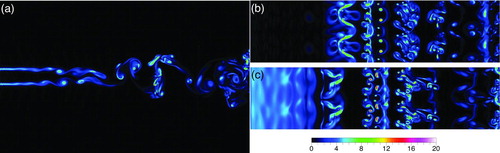
The flow-field is illustrated in Figure 2. Instantaneous contours of vorticity magnitude are shown at z = 0, y = 0, and y/D = 0.5 in panels (a), (b), and (c), respectively. The contours in Figure 2a show a typical Karman vortex street in which vortices pair and roll up, and after which three-dimensional instability ensues resulting in the appearance of vortex tubes and the breakdown of regular vortices Roshko (1954). As the vortices grow, they bring hot and cool fluids—as well as DBP-laden fluid and DBP-free fluid—into contact. The three-dimensionality of the flow, evidenced in Figures 2b and c, suggests that mixing in the span-wise direction begins by x/D = 5. The contours also show that the shear layers merge by x/D = 8.

Figure 3 FIG. 3 Cross-stream profiles of the time-averaged (a) normalized temperature,

, and (b) normalized DBP mass fraction,

.

The manner in which the temperature and species fields evolve as the flow develops significantly affects particle formation. The growth of molecular clusters due to collisions with single molecules drives nucleation. Once an energy barrier is surmounted stable clusters form. If not then the cluster disassociates into its constituent molecules (Friedlander 2000). These collisions are proportional to the concentration and the kinetic energy is proportional to the temperature. The temperature is nondimensionalized via θ =(T−T_∞)/(T_o−T_∞) and the DBP mass fraction is normalized via . Cross-stream profiles of the time-averaged temperature and DBP mass fraction, are shown in Figure 3. The profiles are quite similar and show that between x/D = 2 and x/D = 4 transport is primarily due to diffusion as the quantities diffuse across the height of the wake. Differences in diffusive transport are evident even at x/D = 2. If one looks at the region near the interface of the two streams, y/D = ±0.5, it is evident that the gradients (in the cross-stream y-direction) are sharper in the mass-fraction, , than in the temperature This is due to the non-unity Lewis number, Le = 5.43. This dissimilar molecular scale transport results in high concentration at a lower temperature and is what Clement (1985) refers to in describing nucleation when the Lewis number is unity. With Le = 1, the profiles would almost be identical, which would decrease the saturation ratio (given by Equation (7(7) )), a measure of the driving force toward particle formation. Between x/D = 4 and x/D = 8, large-scale convective transport becomes significant. For example, at the centerline y/D = 0 the temperature drops by roughly 75%. Similarly, the nondimensional mass fraction decreases from at x/D = 4 to at x/D = 8. Further downstream, the wake grows as the faster co-flowing fluid entrains and dilutes the DBP-laden vapor. The result is by x/D = 16, the temperature and concentration are within 12% of the values in the co-flowing streams. The effect of a non-unity Lewis number is most obvious in the laminar region of the flow. Once turbulent mixing becomes more prominent, the gradients in temperature and concentration drive augment nucleation and the importance of the Lewis number diminishes slightly. However, it still remains important.

3.5. Particle Nucleation Rate

Generally, the dynamics of the temperature and the mass-fraction are such that the saturation ratio increases as the jet travels downstream. This is primarily through cooling and dilution. The saturation ratio is a function of temperature, mass-fraction, and the saturation mole fraction, x_sat, for DBP. It is the latter that causes the significant changes in S. A scatter plot of the instantaneous nucleation rate, log₁₀(J), versus saturation ratio, S, is shown in Figure 4a. The data show that the nucleation rate increases with increasing saturation ratio, though not linearly. Nucleation rates above J = 1 particle/(m³·s) require the saturation ratio to be higher than approximately S = 20, which is 200% higher than the inlet condition (at x/D = 0). A large saturation ratio value indicates a location that has departed far from thermodynamic equilibrium. A return to equilibrium entails a phase change of an increasing amount of mass or high nucleation rate. An increasingly large departure from equilibrium is needed for higher nucleation rates to occur. Large-scale convective transport and molecular mixing, evidenced in Figure 3, lead to saturation ratios in excess of S = 1500, which in turn leads to nucleation rates as high as J = 1×10¹⁷ particles/(m³·s). Additionally, it is important to note that for a given nucleation rate there are a range of saturation ratio values. And, in fact, there are multiple conditions in the flow that can produce the same nucleation rate.

Figure 4 FIG. 4 (a) Scatter plot of the nucleation rate, log₁₀(J), versus saturation ratio, S, and (b) scatter plot of the normalized temperature, θ, versus normalized mass-fraction, φ, with lines of constant critical diameter, d_c. (Color figure available online.)

Figure 5 FIG. 5 Contours of the nucleation rate particles/(m³·s): (a) instantaneous log₁₀(J) on plane z = 0, at time t* = 81.79, and (b) time-averaged,

. (Color figure available online.)

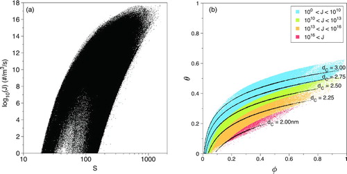
A slightly different view of the nucleation dynamics is presented in the temperature mass-fraction scatter plot shown in Figure 4b. This reflects how various combinations of temperature and mass-fraction result in the nucleation of particles of various sizes. As the wake travels downstream, the fluid emanating from the nozzle traverses trajectories that begin at the upper right (hot and concentrated) and end near the lower left (cool and dilute). The figure shows that the critical particle sizes vary from d_p = 2 nm to d_p = 3 nm. The rate at which the small 2 nm diameter particles form is some 5–7 orders of magnitude greater than the rate at which the larger 3 nm diameter particles form. The figure also shows that as the temperature decreases, the particle diameter decreases as well (Shneidman 1995). At high mass-fractions, changes in the temperature have a more significant effect on the nucleation rate as compared to low mass-fractions. The reason for this conclusion can be seen by fixing the mass-fraction at a high value (e.g., φ = 0.6) and decreasing the temperature. As the temperature decreases, you will pass through lines of constant nucleation rate; the rate increasing a number of orders of magnitude. Conversely, at very low mass-fraction values (e.g., φ = 0.2), a similar decrease in temperature yields a smaller increase in nucleation rate. Similarly, at low temperatures, changes in the mass-fraction have a more substantial effect on the nucleation rate, compared to the same changes at high temperatures. In laminar flows, molecular transport is the mechanism by which the fluid elements traverse this space, illustrating the importance of the Lewis number. A Lewis number of unity, Le = 1, means that changes in the temperature are met with commensurate changes in the mass-fraction. With Le = 5.38, the rate at which the fluid cools is greater than the rate at which it is diluted, resulting in greater saturation ratios than in the Le = 1 scenario. That is the rate-of-descent through Figure 4b is more steep with Le = 5.38 than it is with Le = 1, yielding more nucleation (Clement 1985).

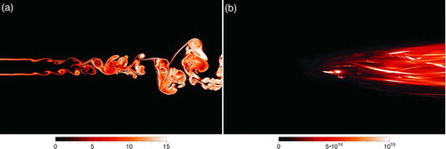
Contours of the nucleation rate are shown in Figure 5; two views are presented. The first contains instantaneous nucleation, log(J), at time t* = 82 shown in Figure 5a and the second contains the time-averaged nucleation rate, , shown in Figure 5b. The log  is shown purely to elucidate how particle nucleation occurs as the flow develops. This is because the values have significant variation (10² < J < 10¹⁸) and the high values would completely obfuscate the dynamics within the developing wake. The instantaneous contours show that within the first four diameters, nucleation is confined to the interface of the two streams where molecular diffusive transport is the dominant mechanism. Again, this is enhanced by the non-unity Lewis number (Clement 1985). However, as the vortices form and roll-up and the two streams mix (between x/D = 4 and x/D = 10), nucleation across the width of the wake increases significantly. Molecular transport is greatly aided by large-scale convective transport, which brings the faster-moving, cooler, DBP-free fluid into contact with the slower-moving, hotter, DBP-laden fluid. As a result, the nucleation rate is as high as J = 10¹⁴ particles/(m³·s) across the height of the wake by x/D = 8. The flow travels further downstream, becomes turbulent, and both the nucleation rate and the extent of the flow in which nucleation is taking place increase. This reflects the merging of the shear-layers and the large-scale mixing of the hot, low-speed, DBP-laden fluid, with the cooler, DBP-free high-speed stream. Instead of thin bands of nucleation, there are “large blobs” of gas that are now producing DBP nanoparticles. If one considers the time-averaged nucleation rate, shown in Figure 5b, it is clear that nucleation prior to the collapse of the wake potential core is insignificant compared to the postcollapse nucleation field. Between x/D = 8 and x/D = 16, the nucleation rate increases slightly, but the greater change is the growth or spreading of the wake and the accompanying spread of nucleation. Across the height of the wake, from −2.5<y/D < 2.5, the nucleation rate is fairly uniform with values between J = 10¹⁴ and J = 10¹⁵.

Figure 6 FIG. 6 Scatter plots of (a) the normalized, filtered temperature, ⟨θ⟩_L, versus exact normalized temperature, θ, and (b) the normalized, filtered DBP mass-fraction, ⟨φ⟩_L, versus the exact normalized DBP mass fraction, φ, at time t* = 81.79. The line of equal values is shown in gray. (Color figure available online.)

3.6. Analysis of the SGS Nucleation

Nucleation is sensitive to temperature and concentration fluctuations. This is observed by considering the dependence on the square of the mass-fraction, Y, and the exponential temperature dependence in Equation (5(5) ). Understanding the effects of the fluctuations is key to improving the predictive ability of modeling tools. Here we define large or resolved-scale quantities and small or unresolved subgrid-scale quantities in a manner consistent with large eddy simulation (Aldama 1990; Germano 1992). The large or resolved-scale variables are obtained via (9) where is the spatial filter function and is the spatially filtered quantity (Germano 1992). The filter employed here is the commonly employed top-hat or “moving average” filter with width Δ_F (Aldama 1990; Garrick 1995). The flows considered here are of variable density, which means that density-weighted or Favre-filtered quantities must be used. These quantities are defined via (10) and fluctuations are defined as A′ = A−⟨A⟩_L (Jaberi et al. 1999). To elucidate the effects of the unresolved and small-scale fluctuations on nucleation, we compute the nucleation rate based on the resolved-scale quantities and obtain the SGS component via subtraction. The large-scale nucleation rate, J^F_L is given by (11) where S^F_L, d^F_cL, and σ^F_L are the resolved-scale saturation ratio, critical diameter, and surface tension, respectively, obtained using the filtered temperature, mass-fraction, density, and pressure. The SGS nucleation rate is defined as the difference between the two rates, J^SGS_L = J−J^F_L. Negative values of J^SGS indicate that the SGS interactions act to decrease particle nucleation, while positive values of J^SGS indicate that the interactions act to increase particle nucleation. We utilize two filter widths in this study. In case 1, the DNS data is filtered using a filter width of Δ_F = 4×Δ_DNS and in case 2 a value of Δ_F = 8×Δ_DNS is utilized, where Δ_DNS is the grid spacing employed in the DNS. These values are chosen as they compare favorably with resolutions used for LES of similar flows (Colucci et al. 1998; Garrick et al. 1999; Gicquel et al. 2002; Givi 2006).

Figure 7 FIG. 7 Scatter plots of the saturation ratio based on the filtered temperature and DBP mass-fraction, S^F_L, versus the exact saturation ratio, S, at time t* = 81.79: (a) case 1 and (b) case 2. The line of equal values is shown in gray.

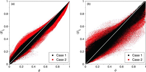
Scatter plots of the normalized, filtered temperature, ⟨θ⟩_L, and mass-fraction, ⟨φ⟩_L, versus their exact counterparts (θ and φ) are shown in Figure 6. Figure 6a shows that for high temperatures, the filtered value is lower than the exact, ⟨θ⟩_L < θ. At low temperatures, the trend reverses and the filtered value is generally higher than the exact, ⟨θ⟩_L > θ. This trend is more pronounced when the larger filter width is used (in case 2). Figure 6b shows a similar trend for the mass-fraction. These results indicate that the filtering acts to create a more homogeneous dependent variable field.

Scatter plots of the saturation ratio obtained using the filtered temperature and mass-fraction, S^F_L, versus the exact saturation ratio, S, are shown in Figure 7. Figure 7a shows that for case 1, at low values of saturation ratios, S^F_L > S. However, as S increases, this trend reverses. For example, at S = 200, S^F_L ranges from S^F_L = 50 to S^F_L = 600, with the majority of values above S^F_L = 200. Conversely, at S = 600, the majority of the values lie between S^F_L = 250 and S^F_L = 700. Again, with a small number of higher outliers. Similar results for case 2 are presented in Figure 7b. Here, as in case 1, use of the filtered temperature and mass-fraction tends to lead to an over-prediction of the lowest saturation ratio values and an under-prediction at the higher saturation ratio values. The increased filter-width used in case 2 is responsible for the complete absence of values above S^F_L = 900. Mixing—diffusion, large-scale convective, or as mimicked by the spatial filtering—creates a more homogeneous-dependent variable field and provides fewer opportunities for the system to be as far from thermodynamic equilibrium. Thus, as small-scale fluctuations are removed, the highest saturation ratio values are greatly reduced.

A comparison between the nucleation rate J^F_L and the exact nucleation rate J for case 1 is shown in Figure 8a. While the maximum value of J^F_L is slightly lower than the exact nucleation rate, the lower values tend to be over-predicted. In the majority of the flow, where nucleation rates are relatively low, the flow is not yet well mixed. The use of the spatially filtered dependent variables mimics more mixed temperature and mass-fraction fields, most often resulting in greatly increased nucleation rates. The highest nucleation rates only occur once transition to turbulence begins. Here, the flow is well mixed and the filtering process affects the temperature and mass-fraction fields less. This results in less scatter at the highest nucleation rate values. For example, when the exact nucleation rate is J = 10² particles/(m³·s), the nucleation rate based on the filtered temperature and mass-fraction varies between J^F_L = 1 and J^F_L = 10¹⁴ particles/(m³·s). This shows an opportunity for an over-prediction of as much as 12 orders of magnitude. However, this trend reverses as the nucleation rate increases. At higher nucleation rates, the degree of variability decreases and the trend is for J^F_L to be lower than the exact rate J. At a nucleation rate of J = 10¹⁵ particles/(m³·s), the nucleation rate based on the filtered temperature and mass-fraction varies between J^F_L = 10¹¹ particles/(m³·s) and J^F_L = 10¹⁶ particles/(m³·s). When the filter-width is increased, the trends are similar but the magnitudes are increased. The results for case 2 are shown in Figure 8b. The nonlinear nature of Equations (5(5) ) and (7(7) ) can be seen by examining the correlation coefficient values for the nucleation rate. The definition used here is the covariance of the variables in question (e.g., J and J^F_L) divided by the product of their standard deviations, (Hayter 1996). The correlation coefficient for the nucleation rate for case 1 is r = 0.60. The increased filter width of case 2 shows a much larger effect, yielding a correlation coefficient of r = 0.39 for the nucleation rate. These results suggest that the nucleation rate is quite sensitive to small fluctuations in temperature and mass-fraction.

Figure 8 FIG. 8 Scatter plots of nucleation rate based on the filtered temperature and DBP mass-fraction, J^F_L, versus exact nucleation rate, J, at time t* = 81.79: (a) case 1 and (b) case 2. The line of equal values is shown in gray.

Figure 9 FIG. 9 Probability density function of the subgrid-scale nucleation rate J^SGS_L for case 2.

Probability density functions (PDFs) of the SGS nucleation rate J^SGS are constructed to provide a more quantitative description of the SGS interactions. The SGS nucleation values are separated into positive and negative values for ease of presentation. Negative J^SGS values (J^SGS < 0) mean that the unresolved SGS interactions act to reduce the nucleation of nanoparticles while positive values (J^SGS > 0) mean that the unresolved SGS interactions act to increase nanoparticle nucleation. The PDF of the SGS nucleation rate for case 2 is shown in Figure 9. The PDF shows that while there are more than twice as many negative SGS values (J^SGS < 0) as there are positive SGS values (J^SGS > 0), the positive contributions are as much as two orders of magnitude greater than the negative contributions. This PDF provides a comprehensive overview of the effect of the unresolved temperature and mass-fraction interactions on homogeneous nucleation. The SGS interactions predominantly act to increase nucleation.

3.7. Sensitivity of Nucleation to Scalar Fluctuations

To elucidate more clearly how changes or fluctuations in the fluid temperature and DBP mass-fraction affect the nucleation rate, PDFs of the SGS nucleation rate conditioned on the normalized temperature fluctuation, θ′ = θ−⟨θ⟩_L, and the normalized DBP mass-fraction fluctuation, φ′ = φ−⟨φ⟩_L, are constructed (note: if the SGS interactions did not affect the nucleation rate, then J^SGS would be zero and the scatter shown in Figures 7 and 8 would be straight lines). The fluctuations are such that positive values of θ′ and φ′ reflect small-scale heating and increased concentration, respectively, while negative values reflect small-scale cooling and dilution.

PDFs of the SGS nucleation rate conditioned on the temperature fluctuation θ′ for case 2 are presented in Figure 10. Again, for clarity, the SGS nucleation is separated into positive and negative contributions. Positive SGS nucleation values are shown in Figure 10a and negative SGS nucleation values are shown in Figure 10b. If we look to where the SGS interactions act to decrease nucleation, Figure 10a shows that locations where the temperature is increased by up to 10% are most prominent while locations where the temperature is decreased by up to 10% decrease the nucleation rate by the highest magnitude, J^SGS = −1.6×10¹² particles/(m³·s). Turning to the PDF of the positive SGS nucleation rate, Figure 10b suggests that locations where SGS cooling decreases the temperature by up to 10% result in SGS nucleation rates as high as J^SGS = 10¹⁴, while locations where SGS heating increases the temperature by up to 10% result in SGS nucleation rates as high as J^SGS = 10¹², i.e., SGS cooling results in the most significant change to the nucleation rate. This is expected as a decrease in temperature means a decrease in the kinetic energy of the DBP molecules and therefore an increase in the number of stable DBP clusters available for future growth. Additionally, a decrease in temperature results in a lower DBP saturation mole fraction, x_sat, which allows super-saturation (and thus nucleation) to occur at lower DBP vapor concentrations.

Figure 10 FIG. 10 Probability density functions of the magnitude of the SGS nucleation rate, J^SGS_L, conditioned on the normalized temperature fluctuation, θ′ (case 2): (a) J^SGS_L < 0 and (b) J^SGS_L > 0.

Figure 11 FIG. 11 Probability density functions of the magnitude of the SGS nucleation rate, J^SGS_L, conditioned on the normalized mass-fraction fluctuation, φ′ (case 2): (a) J^SGS_L < 0 and (b) J^SGS_L > 0.

PDFs of the SGS nucleation rate are also conditioned on the DBP mass-fraction fluctuation and the results for case 2 are presented in Figure 11. Turning our attention to locations where the SGS nucleation is negative (J^SGS < 0), shown in Figure 11a, a fluctuation corresponding to a 10% increase in mass-fraction is the most frequent value, corresponding to J^SGS = 1.6×10¹² particles/(m³·s). However, there is a cluster of values corresponding to J^SGS = 6.3×10¹², the most prominent of which occurs when the fluctuation decreases the normalized DBP mass-fraction by as much as 10%. Looking back at Figure 4, the data suggest that if such changes in the mass-fraction result in such large SGS nucleation values, the mass-fraction itself must be relatively low—somewhere in the range 0.01 < φ < 0.15. The PDFs presented in Figure 11b show that locations where SGS dilution occurs act contribute the most to positive SGS nucleation. The reason for this is not obvious, considering that a decrease in DBP mass-fraction (while the temperature is constant) results in a decrease in the saturation ratio and therefore a decrease in the nucleation rate. However, the data presented in Figure 4 suggests that if the decrease in mass-fraction is accompanied by a decrease in temperature then the nucleation rate does indeed increase. At high DBP mass-fractions the magnitude of the temperature-decrease needed is less than that needed at lower mass-fractions. More simply put, mixing that results in dilution and cooling yields more nucleation when the mass-fraction is high.

4. CONCLUSIONS

Direct numerical simulation (DNS) of the nucleation of dibutyl-pthalate (DBP) particles in a turbulent wake was performed. Classical nucleation theory (CNT) is employed to model the formation of particles from DBP vapor. An a priori analysis of the DNS data was performed to elucidate the effects of unresolved or subgrid-scale (SGS) interactions on nanoparticle nucleation. The temperature, pressure, density, and mass-fraction fields are spatially filtered—using two filter-widths—and the saturation ratio and nucleation rates are computed. Those quantities are compared to the exact saturation ratio and nucleation rate, thus isolating the effects of SGS scalar–scalar interactions on nanoparticle nucleation. As the filter-width is increased, so is the magnitude of the unresolved or SGS terms.

The simulation data shows that nucleation initially occurs at the interface of the slow, hot, DBP-laden stream, and the cooler, high-speed DBP-free stream. This is where diffusion-driven mixing occurs resulting in an increase in the saturation ratio. However, as the flow develops convective mixing or entrainment becomes the dominant mixing mechanism and the nucleation rate increases significantly and is no longer confined to the shear layers. So, while shear layer nucleation is indeed present, the increase in nucleation rate—once the potential core collapses—is several orders of magnitude greater (Lesniewski and Friendlander 1998). Considering the nucleation rates in the temperature, mass-fraction space suggests that a Lewis number of unity (Le=1) results in reduced nucleation as postulated by Clement (1985). The results also show that the effects of the unresolved or SGS fluctuations are quite significant, though decreasingly so as the nucleation rate increases. At low nucleation rates, the fluctuations primarily serve to decrease particle formation, while at the highest nucleation rates, the SGS fluctuations act to increase particle formation. And, statistical analyses reveal that vapor dilution and cooling occurs where the SGS fluctuations increase.

Analysis of the DNS dataset suggests that fluid turbulence, simulation resolution, and fluctuations can be as significant as nucleation theories (CNT, scaled nucleation theory, etc.) in the accuracy of predicting particle formation rates. Additionally, the importance of molecular mixing—vis a vis the Lewis number—on nucleation suggests that modeling approaches such as gradient-diffusion type closures, which employ unity Lewis number assumptions can significantly under-predict particle formation in the transition region of turbulent flows (Di Veroli and Rigopoulos 2011). As nucleation tends to scavenge vapor via condensation, and affect subsequent particle formation and growth rates, careful modeling is required and probability-based approaches that are able to account for unequal diffusivities can be of great utility (Viswanathan et al. 2011).

Support for this work was provided by the Digital Technology Center at the University of Minnesota. Computational resources were provided by the Minnesota Supercomputing Institute.