Development of a Real-Time, In-Situ Particle Sizing Technique: Real-Time Light Transmission Spectroscopy (RTLTS)

Abstract

We developed an improved particle measurement spectroscopic technique, real-time laser transmission spectroscopy (RTLTS), to detect the number-weighted distribution of particles in real time. The measurement system used a deuterium–tungsten lamp for the light source and a spectrometer as the detector. The operating wavelength range was 300–810 nm. To obtain a physically reasonable number concentration from the experimental results, a sequential regularization method was used during the calculations. To verify the feasibility and reliability of RTLTS, the number-weighted distribution of polystyrene particle suspensions was determined over diameters ranging from 0.005 to 2.000 μm in 0.005-μm increments. The measured concentration error was 0.67–32.67%. A mean diameter of the smallest particle we had detected was 0.09 μm, with a 16% oversizing. The measurable concentration range was ∼10⁸ #/cc to ∼10¹¹ #/cc for 0.895-μm-diameter particles. The measurable concentration range could be adjusted simply by changing the system configuration. This technique is available for both waterborne and airborne particles.

Copyright 2013 American Association for Aerosol Research

1. INTRODUCTION

Optical systems offer the advantages of real-time, in-situ measurements for particulate systems. Dynamic light scattering (DLS) (Berne and Pecora 1976; Pecora 1985), laser-induced incandescence (LII) (Eckbreth 1977; Melton 1984), and the light (or laser) extinction method (LEM) are examples of optical particle measurement techniques (Zollars 1980; Boufendi et al. 1992). However, these methods are unable to measure the number-weighted distribution of the particle directly. Additionally, these techniques can be expensive and complicated; for example, LII and LEM require additional quantification conversion, and DLS requires elaborate dilution (Park et al. 2010; Yoon et al. 2011). Some particle measurement techniques using light extinction spectrum can be used to measure the number-weighted distribution of particles without additional quantification procedures (Jones et al. 1994; Wang and Hallett 1996; Ferri et al. 1997; Müller et al. 1999). However, it demands both elaborate scattering light detection and data processes, because ill-posed problem could arise.

A particle measurement technique using light extinction spectrum, laser transmission spectroscopy (LTS) named by Li et al. (2010, 2011) was developed to measure cell sizes or deoxyribonucleic acid (DNA) in some biological systems. LTS has the advantage of high accuracy, in addition to the ability to determine particle distributions over a wide range of concentrations and particle sizes. Furthermore, the resolution of LTS can be enhanced on demand because its resolution is proportional to the beam path length due to its dependency on the Beer–Lambert law (Seon et al. 2007). However, conventional LTS requires very long scan times because the light extinction must be measured for each and every wavelength individually. Furthermore, the optical system required for LTS uses expensive tunable lasers.

A real-time measurement technique is needed for other research fields in which the particle size or number concentration changes rapidly. Automotive engineering could be one such application that requires a real-time measurement technique. The exhaust regulations for the automotive industry have become increasingly strict, particularly for diesel engines and diesel particulate matter emission. Moreover, diesel particulate regulations have changed from a mass basis to a number concentration basis because of the harmful nature of nanoparticles (Kittelson 1998; Kasper 2008). There has been significant interest in developing real-time measurement techniques that measure particulate matter in exhaust because these emissions have been shown to be sensitive to engine operating conditions (Witze et al. 2004; Wei and Rooney 2010; Johnson 2011; Yoon et al. 2011).

In this study, we developed a real-time LTS (RTLTS) to measure the number-weighted distributions of waterborne and airborne particles. We could not obtain results instantly because of the data processing time; thus, RTLTS cannot be applied to a closed-loop feedback system. However, the transient behavior of the target can be recorded at a very fine time resolution (4 ms), regardless of the data processing time. Therefore, RTLTS is a real-time measurement technique (not including data processing) applicable for analyzing the transient behaviors of particle concentrations. We also emphasized that the purpose of this study is not to improve the accuracy, but to develop a real-time measurement.

2. THEORY

2.1. LTS Theory

LTS is a particle measurement technique based on the Beer–Lambert law, which explains the light extinction phenomenon by particles or gaseous molecules (Li et al. 2010):

T, P, α, z, and λ refer to the transmittance, intensity, extinction coefficient, beam path length, and wavelength, respectively. If the light extinction occurs by spherical particles of various size, and the light wavelength of the source is not monochromatic, then the extinction coefficient, α, can be expressed as

where σ is the extinction cross-section (the amount of light extinction), n is the number concentration, and d is the size of the particle.

Two tunable lasers and optical cells were used in the measurement system of Li et al. (2010). They obtained four data outputs for each case, and the transmittance T was calculated by the reduction of a complex fraction. For the measurement system used for this study, there were two data outputs from a simplified system, consisting of a single light source and two optical cells. In this case, the transmittance, T, can be expressed as follows:

where ϵ is the detector efficiency, T_p is transmittance of particle, T_f is transmittance of fluid, and P _source is the intensity of light source. If the extinction cross-section, σ, is substituted by Mie scattering simulation data during data processing, and the extinction coefficient, α, is obtained from the experimental results, then the number concentration of particles, n, can be calculated. The variables α, σ, and n, are given below in matrix form:

The number-weighted particle distribution can be obtained if matrix inversion is performed to calculate n.

A precise simulation of the extinction cross-section, σ, is important for accurate results. Some Mie-scattering simulation programs for extinction cross-section determination have already been developed (Felske et al. 1983; Laven 2011; Zakharov 2011; Prahl 2012). Among them, we chose Mieplot 4.3 by Laven (2011), which supports the import of external refractive indices. Its reliability has been verified by many researchers (Riley et al. 2004; Husted et al. 2009; Shen and Wang 2010; Kinnunen et al. 2011). The refractive index value of polystyrene was adopted from Palik (1991).

2.2. Regularization Methods

The matrix inversion problem involved in this work is considered to be an ill-posed problem in its current form. Ill-posed problems appear frequently when doing matrix inversions. Even if no error exists, the wrong solution can be obtained because the inversion matrices are not identical. If a problem demands large-scale calculations, like the ones required for this study, then excessive change could occur regarding the solution. Thus, it is almost impossible to obtain a reasonable solution of the matrix inversion problem without any “trick,” when experiment and simulation are both involved. In this case, the regularization method was used to obtain physically reasonable and reliable solutions.

There are various software codes available to perform regularization. Some researchers make their own codes freely available to other researchers (Weese 1992; Hansen 1994, 2007, Schmidt et al. 2007). In particular, Hansen (1994) made available a MATLAB package, “Regularization Tools,” which is composed of various regularization methods for general-purpose use. Nagy et al. (2004) confirmed that the Regularization Tools software could be used for image-field restoration and real applications.

Among the regularization methods, we chose the Tikhonov regularization and maximum entropy regularization. The inversion problem given below is used to explain the procedures involved with these methods.

A, b, and x correspond to the database that is already known, the experimental data, and the solution, respectively. In this study, A, b, and x are substituted for , and n, respectively. For easier understanding of regularization formulas, we use A, b, and x which are common notations of matrix inversion problem. In practice, the optical noise, such as the electrical noise of the detector, poor optical alignment, and changes in the refractive indices of medium due to temperature variation and intensity fluctuations of light source, must be accounted for. The noise factor for our experimental data is written as b + . Thus,

If there is noise, , then the error in the solution can never be eliminated. In some cases, small noise can result in a very large error in the solution. With the regularization method, a “regularization term” is used to minimize the noise and error. The type of regularization method used was determined based on the form and algorithm of the regularization term. Tikhonov and Arsenin (1977) suggested a formula for regularization, referred to as Tikhonov regularization, given below:

where x _β , x ₀, and β represent the regularization solution, the initial value (supposition of the solution), and the regularization parameter, respectively. The regularization parameter, β, determines the weight of the initial value, x ₀, and minimizes the noise.

Likewise, the maximum entropy regularization is written as shown in Equation (9) (Fletcher 1981; Hansen 1994):

This maximum entropy equation exhibits slow convergence, so the use of a modified form is recommended, similar to the one shown in Equation (10) (Chiang et al. 2005b):

The modified form of the maximum entropy functional (Equation (10)) is equivalent to Equation (9), and it is also analogous to the Tikhonov functional in its properties (Eggermont 1993; Engl and Landl 1993). This transformed functional not only possesses the non-negativity constraint of the regularized solution for x _i by virtue of the natural logarithm, but also obtains enhanced stability and convergence from the Tikhonov functional (Chiang et al. 2005b).

The differences between the Tikhonov and maximum entropy regularization are the regularization term and the existence of the nonzero constraint. Although the Tikhonov regularization is one of the easiest, more widely used methods, it may present solutions with values below zero; therefore, for many physical applications, this method is not practical and is used directly. However, Calvetti et al. (2004) and Nagy and Strakos (2000) developed nonzero Tikhonov regularization codes and successfully applied them to image restoration. Unfortunately, for this work, these codes are not applicable. Although a blurred image can be used as the initial value, x ₀, in an image restoration field, for our study, we do not know the initial value of the particle concentration when doing the particle measurement test. In this type of situation, maximum entropy regularization can be used instead. Maximum entropy regularization provides a very accurate, nonzero, constrained solution due to iterative calculations.

In this study, we used both Tikhonov and maximum entropy regularization, sequentially, as suggested by researchers in similar application fields (Chiang et al. 2005a,b). Sequential regularization requires using the solution of the Tikhonov regularization as the initial value for maximum entropy regularization. Sequential regularization supplies the solution quickly, even if the data have a low signal-to-noise ratio. In our simulation test, this sequential regularization successfully recovers the spectrum under random virtual noise of 50dB signal-to-noise ratio. We modified the MATLAB code to optimize the code provided by Chiang et al. (2005b) because the regularization method demands optimization of the code according to the size and scale of the matrices. The regularization factor β was decided by the L-curve criterion code by Hansen (2007), as Chiang et al. (2005b). Note that the initial value for the Tikhonov regularization was not specified on the assumption that we did not know the number-weighted distribution of the target particles.

3. EXPERIMENT

3.1. Optical System

The influence of Mie scattering increases when the particle diameter is much larger than the wavelength of light. However, the wavelength range for extinction, which is particularly effective, is limited. This phenomenon is observed not only with laser light but also with polychromatic light. (Migliorini et al. 2011). Thus, a system with a wide wavelength range is needed to measure various particle diameters. To produce light over then UV–VIS–IR spectrum simultaneously, we selected a deuterium–tungsten lamp (DH-2000-BAL, Ocean Optics). The light from the lamp was delivered to a charge-coupled device (CCD) sensor, equipped with a spectrometer (USB4000, Ocean Optics) through an antisolarization optical fiber. Figure 1 shows a schematic diagram of the RTLTS system.

FIG. 1 Schematic diagram of the real-time laser transmission spectroscopy (RTLTS) optical system.

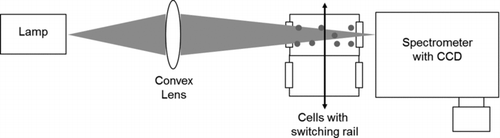
A single convex lens was used for optical alignment to minimize spectrum distortion due to the optical instruments. If the light intensity was insufficient to use the complex lens system, aspheric lenses could be used to obtain a more accurate alignment. For the experiment, two identical optical cells were prepared. UV-fused silica windows were installed on the cells. The difference in transmittance between the two cells was experimentally determined to be <0.1%. One of the cells was filled with deionized water. The other cell was filled with a polystyrene particle suspension. The specific gravity of deionized water was matched to the particle's specific gravity (1.05) using sodium chloride, to prevent sinking or floating of particles. A switching rail was prepared to move the cells oppositely. During the experiment, one cell was used for measurement and the other was used as a reference. The optical beam path length was 2.4 cm.

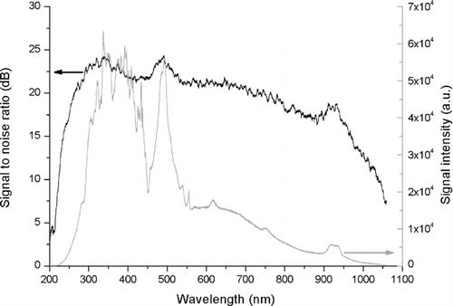
FIG. 2 Response spectrum of the optical system and its signal-to-noise ratio.

3.2. Target Wavelength

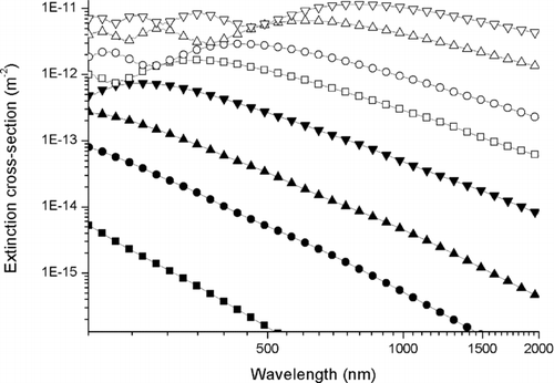
For particle concentration measurements, broadening the target wavelength could potentially extend the measurable particle range. In this study, broadening the target wavelength presented two major drawbacks. First, the time required for regularization would increase. Increasing the size of the calculation matrices increased the calculation time, particularly with the iterative method used in the maximum entropy regularization. Second, the optical system was limited in its spectral coverage. The light intensity detected by the spectrometer for each spectrum was not uniform. This phenomenon attributed to the nonuniformity of the quantum efficiencies and variation in the transmittance or reflectance of the optical instruments. The response spectrum of the optical system and the signal-to-noise ratio are shown in Figure 2. The light intensity of deep UV (λ = 200–300 nm) and NIR (λ = 850–1100 nm) was relatively low for this system; thus, the transmitted light may not be detected in this portion of the spectrum. To decrease the influence of the signal-to-noise ratio, we chose 300–810 nm for the wavelength range. The number of spectral channel contained in this wavelength range was 2089. Figure 3 shows the simulation results of the extinction cross-section to confirm the feasibility of the selected wavelength range. We found that particle diameters of d ≥ 0.5 μm exhibited sufficient light extinction over the entire wavelength range. These particles were expected to be detected easily because the extinction patterns of each particle were distinctly different. In contrast, particles with diameters of d ≤ 0.3 μm have relatively low extinction cross-sections. The maximum value of the extinction cross-sections should exist at shorter wavelengths. Detecting particles with diameters of d = 0.1 μm was expected to be particularly difficult due to the extremely low extinction cross-section. Confusion among small particles was anticipated because their extinction patterns were similar and difficult to distinguish for low signal-to-noise ratios. Fortunately, the spectral resolution of UV optical instruments is generally very narrow. We determined that the smallest particle that we could use was a Spherotech 0.09-μm-diameter particle, which was close to the expected 0.1-μm limit.

FIG. 3 Simulated extinction cross-section of submicron particles by the Mieplot program for diameter d = 0.1(▪), 0.2(•), 0.3(▴), 0.5(▾), 0.75(□), 1.0(○), 1.5(▵), and 2.0(▿) μm polystyrene particles.

3.3. Experimental Conditions

Polystyrene was chosen as the measurement target particle because it is widely used in the diagnosis field (Cross et al. 2010). The particles used in this test were National Institute of Standards and Technology (NIST) Standard Reference Materials (SRMs) and Spherotech polystyrene particles. Generally, NIST SRMs are utilized for calibration of particle measuring instruments because their sizes are thoroughly controlled. We used them to verify the feasibility of RTLTS and to evaluate the linearity of concentration. A diameter error of <0.1% was guaranteed by the manufacturer. For these tests, the particle source (5 wt%) was diluted in various ratios.

In contrast, the Spherotech polystyrene particles were not as precise as the NIST SRM particles. Nevertheless, they can still be utilized for research due to their lognormal diameter spectrum. They were used for our diameter-varying test. It is important to note that when preparing the particle suspension sample for various dilution ratios, the difference in concentration can increase drastically. In this situation, comparisons among each case may be difficult because they have different orders of concentration. For this reason, the Spherotech polystyrene particle samples were prepared to a similar order of concentration (∼5 × 10⁸ #/cc) with respect to each other. This concentration value is under the range of PM concentration of common diesel engine raw exhaust (1.0 × 10⁵ ∼ 1.0 × 10¹⁰ #/cc) (Kittelson 1998). Table 1 lists the details for each test case.

TABLE 1 The particle sample preparation for the test

Particle type	NIST SRM	Spherotec
Mean diameter (μm)	0.895 (model 1690)	0.09, 0.41, 1.23
Dilution ratio	1/150, 1/200, 1/250, 1/1000, 1/2500	1/200∼1/10,000
Signal integration time (ms)	4∼120	4

Checking the response time is essential for the development of “real-time” measurement techniques. A spectrometer detects the signal of the entire target wavelength range simultaneously and has the ability to control its signal integration time. When the light intensity is not sufficient for detection, extending the integration time increases the signal and vice versa. Our test began with the shortest integration time, 4 ms. The integration time was extended to 120 ms when excessive extinction was detected.

4. RESULTS

4.1. NIST SRM Polystyrene Particles

One of the particle suspensions used in this experiment was the NIST SRM 1690 polystyrene particle suspension. The manufacturer guarantees an average diameter of d = 0.895 μm with an error of <0.008 μm. To verify the success or failure of RTLTS, the extinction coefficient, α, of the experiment was compared with the Mieplot simulation (Figure 4).

FIG. 4 A comparison of simulated extinction coefficient (dashed line) with experimental result (solid line) for diameter d = 0.895 μm, NIST SRM polystyrene particles, with a dilution ratio 1/250. Note that the results have been normalized. (Color figure available online.)

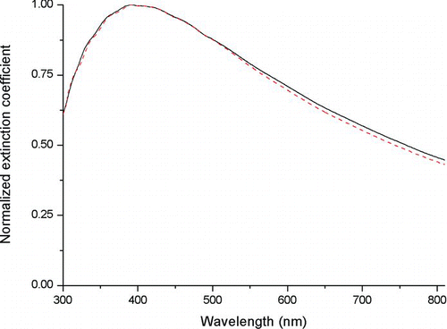
The values of the extinction coefficient, α, can vary with the particle concentration; thus, they were normalized by their maximum value for comparison. The comparison indicated good agreement over the wavelength range of λ = 300–500 nm. However, the difference increased as the wavelength became longer. This error was attributed to the optical alignment, which was tuned to λ = 400 nm. As mentioned in Section 3.1, precise alignment and higher quality of the optical system could improve the precision of these results. Figure 5 shows the matrix inversion results from the experimental data of Figure 4. The results show an irrelevant value with respect to the real NIST SRM size of d = 0.895 μm, as expected. The noise of the data significantly affected the results in this case.

FIG. 5 Matrix inversion solution without regularization for 0.895 μm diameter NIST SRM polystyrene particles, with a dilution ratio 1/250.

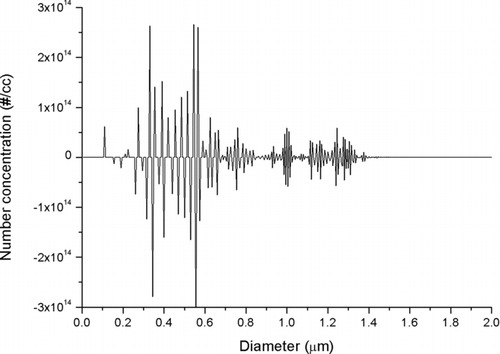
FIG. 6 NIST SRM number weighted distribution result for 0.895 μm diameter polystyrene particles, with dilution ratios of 1/150(□), 1/200(▵), 1/250(○), 1/1000(▿), and 1/2500(×). The manufacturer's data (dilution ratio 1/150) was drawn in dashed line. (Color figure available online.)

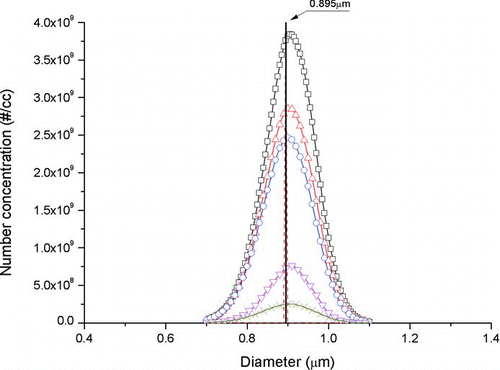
TABLE 2 The linearity analysis of the test using NIST SRM 1690 (d = 0.895 μm, polystyrene particles, dilution ratio 1/150, 1/200, 1/250, 1/1000, and 1/2500)

Dilution ratio	1/150	1/200	1/250	1/1000	1/2500
Mode (μm)	0.905	0.905	0.900	0.910	0.905
Mode number concentration (#/cc)	3.843E+09	2.861E+09	2.467E+09	7.649E+08	2.518E+08
Total number concentration (#/cc)	1.173E+11	9.023E+10	7.839E+10	2.050E+10	8.169E+09
Volume fraction (ppm)	4.597E+04	3.499E+04	3.007E+04	7.927E+03	3.143E+03
Relative dilution ratio	1.000	0.750	0.600	0.150	0.060
Linearity error (@mode number concentration) (%)	–	−0.67	7.00	32.67	10.00
Linearity error (@total number concentration) (%)	–	2.53	11.33	16.67	16.67
Linearity error (@volume fraction) (%)	–	1.47	9.00	14.67	13.33

To solve the inversion problem, sequential regularization was applied to the same data source. The various dilution ratios of 1/150, 1/200, 1/1000, and 1/2500 are shown in Figure 6 for quantitative comparison. The measurement diameter range was 0.005–2.000 μm, in 0.005-μm increments. The number-weighted distribution of the particle suspension was successfully measured. In every test case, 99% of the population was detected in the diameter range of d = 0.895 ± 0.200 μm. The broadening phenomenon was attributed to the optical and electrical noise. The noise can never be removed completely, but it could be reduced by improving the quality of the optical alignment and the instruments used for the experiments. The modes were 0.905, 0.905, 0.900, 0.910, and 0.905 μm in order of decreasing dilution ratio from 1/150 to 1/2500. The reason for the differences in the particle sizes was the gap between the simulation and experimental data. The light extinction of the larger particles was stronger than that of the smaller particles for longer wavelengths. According to the results of Figure 4, the extinction coefficient of the experiment was larger than that of the simulation for a wavelength range of λ = 500–800 nm. This difference could be the cause of the particle size error. The dilution ratio 1/150 was the highest particle concentration case measurable with our RTLTS system. If the particle concentration increased further, then some portion of the signal with a high extinction cross-section would not be detected. On the contrary, the dilution ratio of the 1/2500 case was the lowest concentration detected due to the low signal-to-noise ratio. The measurable particle concentration for our RTLTS system was 8.2 × 10⁹–1.2 × 10¹¹ #/cc within the range of particle concentration commonly observed in diesel engine raw exhaust (Figure 6). This does not correspond to the measurable range of the RTLTS technique, but instead to the limitations of our experimental system. If a detector with better saturation limit and sensitivity is used, the excessive extinction can be avoided and can help widening the measurable range. The sensitivity of the technique can be adjusted by varying the beam path length, according to the Beer–Lambert law. If a multipass cell is used, then the system could be optimized to detect the desirable particle concentration (Seon et al. 2007).

To verify the linearity of RTLTS, the results were rearranged as shown in Table 2. The relative dilution ratio with respect to the dilution ratio of 1/150 is indicated for easy comparison. If the linearity was good, then the ratio of particle concentration showed similar values with respect to the relative dilution ratio. The comparison targets were the mode number concentration, total number concentration, and volume fraction, along with the percentage error. These values are listed in Table 2. The results of the comparisons showed that the largest error of 32.67% occurred for the mode number concentration for a dilution ratio of 1/1000. The linearity error corresponding to the total number concentration for the same case was almost half, that is, 16.67%. This result suggests that the error for the mode number concentration was larger due to poor resolution. We expect that the error will decrease for smaller (<0.005 μm) step increments.

For an easier comparison among each dilution ratio, the normalized graph of Figure 6 is drawn in Figure 7. The normalization was obtained by dividing the data of Figure 6 by each of relative dilution ratio and mode number concentration at 1/150 case which were indicated in Table 2. In the case of dilution ratio 1/1000, the error at mode diameter was found more than 30%, as shown in Table 2. The normalized number concentration of 1/150 and 1/200 case showed similar distribution. On the other hand, 1/250 and 1/2500 case indicated generally higher normalized concentration. These consistent errors could be caused by the inadequate handling during dilution procedure.

FIG. 7 Normalized concentration for NIST SRM 0.895 μm diameter polystyrene particles, with dilution ratios of 1/150(□), 1/200(Δ), 1/250(○), 1/1000(▿), and 1/2500(×). (Color figure available online.)

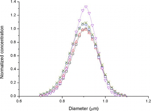
TABLE 3 The size and dispersion data of test particles provided by the manufacturers

Manufacturer	Spherotec			NIST
Model	PP-10-10	PP-05-10	PP-008-10	SRM 1690
Mean diameter (μm)	1.23	0.41	0.09	0.895
Dispersion range (μm)	1.00∼1.49	0.40∼0.60	0.05∼0.10	0.887∼0.903

4.2. Spherotech Polystyrene Particles

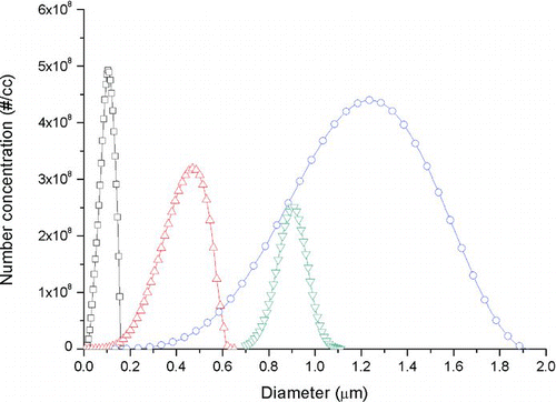
The Spherotech polystyrene particles were used for various diameter tests. For this test, we chose particles with mean diameters of 0.09, 0.41, and 1.23 μm. Unlike the NIST SRM particles, the Spherotech particles do not have a specific certification, but the manufacturer supplies the dispersion range of the particles, which is listed in Table 3. Figure 8 shows the test results using Spherotech particles and a NIST SRM at a dilution ratio of 1/2500. The number-weighted distribution measured by RTLTS was spread over a wide range, compared with the range provided in the manufacturer's data. This result is attributed to insufficient noise filtering, similar to that shown in Section 4.1. The Spherotech 1.23-μm particles showed a wide dispersion range compared with other cases because the manufacturer provided a roughly separated product. The mode diameter of the Spherotech 1.23-μm particles showed no difference with respect to the manufacturer's mean diameter data. However, the diameters of the 0.41- and 0.09-μm particles were 14 and 16% larger, respectively, compared with the values indicated by the manufacturer's data. One of the major sources of error was attributed to the low resolution of the particle size. As the target particle becomes smaller, the step size of the measurement technique has to become smaller as well, to reduce the error. Many commercial particle detectors use a logarithmic step for this reason. We decided to keep the step size at 0.005 μm to ensure that the sources of error are known in the early stages of the test, but it will be modified properly in the application step.

FIG. 8 Spherotec and NIST SRM number weighted distribution result for diameter d = 0.09(□), 0.41(Δ), 1.23(○), and 0.895(▽) μm polystyrene particles, with dilution ratios 1/200∼1/10000. (Color figure available online.)

5. CONCLUSION

We developed an improved particle measurement spectroscopic technique, RTLTS, to detect the number-weighted distribution of airborne or waterborne particles in real time. The measurement system used a deuterium-tungsten lamp and spectrometer to realize real-time measurements and reduce the cost. The sequential regularization method was applied using MATLAB code to convert the signals to particle concentration. To verify the feasibility and reliability of RTLTS, two types of precision polystyrene particles were diluted with deionized water and the concentration was measured. The wavelength range selected was λ = 300–810 nm. Particles were detected from d = 0.005–2.000 μm, in 0.005-μm increments. The measurable range was from ∼10⁸ #/cc to ∼10¹¹ #/cc for d = 0.895 μm. This range was dependent on the system composition (saturation limit or sensitivity) and beam-path length. Thus, the range could be adjusted for various applications. The linearity error of various concentrations was 0.67–32.67%. The minimum size of the particles detected was d = 0.09 μm. According to the Mieplot simulation, larger particles with d ≥ 1 μm should have been easy to detect, and smaller particles with d < 0.09 μm should have been difficult to detect. However, smaller particles could be measured if the system is tuned to the UV range to overcome the low signal-to-noise ratio. The response time was 4∼120 ms. Better alignment and an appropriate UV light source would improve the results further.

NOMENCLATURE

A	=	database of matrix inversion
P	=	intensity of light
T	=	transmittance of light
z	=	beam-path length
b	=	experimental data
n	=	number concentration of particle
d	=	diameter of particle
x	=	solution of matrix inversion
xβ	=	solution of regularization
x0	=	initial value of x (supposition of solution)
α	=	extinction coefficient
β	=	regularization parameter
δ	=	noise
ϵ	=	efficiency of detector
λ	=	wavelength
σ	=	extinction cross-section

Acknowledgments

This work was supported by the Low Observable Technology Research Center Program (LO-22) of Defense Acquisition Program Administration and Agency for Defense Development.

REFERENCES

- Berne , B. J. and Pecora , R. 1976 . Dynamic Light Scattering: With Applications to Chemistry, Biology, and Physics , New York : Wiley .
- Boufendi , L. , Plain , A. , Blondeau , J. P. , Bouchoule , A. , Laure , C. and Toogood , M. 1992 . Measurements of Particle-Size Kinetics from Nanometer to Micrometer Scale in a Low-Pressure Argon-Silane Radiofrequency Discharge . Appl. Phys. Lett. , 60 : 169 – 171 .
- Calvetti , D. , Lewis , B. , Reichel , L. and Sgallari , F. 2004 . Tikhonov Regularization with Nonnegativity Constraint . Electron. T Numer. Ana. , 18 : 153 – 173 .
- Chiang , Y. W. , Borbat , P. P. and Freed , J. H. 2005a . The Determination of Pair Distance Distributions by Pulsed ESR Using Tikhonov Regularization . J. Magn. Reson. , 172 : 279 – 295 .
- Chiang , Y. W. , Borbat , P. P. and Freed , J. H. 2005b . Maximum Entropy: A Complement to Tikhonov Regularization for Determination of Pair Distance Distributions by Pulsed ESR . J. Magn. Reson. , 177 : 184 – 196 .
- Cross , E. S. , Onasch , T. B. , Ahern , A. , Wrobel , W. , Slowik , J. G. Olfert , J. 2010 . Soot Particle Studies—Instrument Inter-Comparison—Project Overview . Aerosol Sci. Technol. , 44 : 592 – 611 .
- Eckbreth , A. C. 1977 . Effects of Laser-Modulated Particulate Incandescence on Raman Scattering Diagnostics . J. Appl. Phys. , 48 : 4473 – 4479 .
- Eggermont , P. P. B. 1993 . Maximum-Entropy Regularization for Fredholm Integral-Equations of the 1st Kind . Siam. J. Math. Anal. , 24 : 1557 – 1576 .
- Engl , H. W. and Landl , G. 1993 . Convergence-Rates for Maximum-Entropy Regularization . Siam. J. Numer. Anal. , 30 : 1509 – 1536 .
- Felske , J. D. , Chu , Z. Z. and Ku , J. C. 1983 . Mie Scattering Subroutines (DMBIE and MIEV0): A Comparison of Computational Times . Appl. Optics. , 22 : 2240 – 2241 .
- Ferri , F. , Bassini , A. and Paganini , E. 1997 . Commercial Spectrophotometer for Particle Sizing . Appl. Optics , 36 : 885 – 891 .
- Fletcher , R. 1981 . Practical Methods of Optimization , New York : John Wiley .
- Hansen , P. C. 1994 . REGULARIZATION TOOLS: A Matlab Package for Analysis and Solution of Discrete Ill-Posed Problems . Numer. Algorithms , 6 : 1 – 35 .
- Hansen , P. C. 2007 . Regularization Tools Version 4.0 for Matlab 7.3 . Numer. Algorithms , 46 : 189 – 194 .
- Husted , B. P. , Petersson , P. , Lund , I. and Holmstedt , G. 2009 . Comparison of PIV and PDA Droplet Velocity Measurement Techniques on Two High-Pressure Water Mist Nozzles . Fire Safety J. , 44 : 1030 – 1045 .
- Johnson , T. V. 2011 . Diesel Emissions in Review , Detroit : SAE World Congress . 2011-01-0304
- Jones , M. R. , Curry , B. P. , Brewster , M. Q. and Leong , K. H. 1994 . Inversion of Light-Scattering Measurements for Particle Size and Optical Constants: Theoretical Study . Appl. Optics. , 33 : 4025 – 4034 .
- Kasper , M. 2008 . Characterisation of the Second Generation PMP “Golden Instrument” , Detroit : SAE World Congress . paper no. 2008-01-1177
- Kinnunen , M. , Kauppila , A. , Karmenyan , A. and Myllyla , R. 2011 . Effect of the Size and Shape of a Red Blood Cell on Elastic Light Scattering Properties at the Single-Cell Level . Biomed. Opt. Express , 2 : 1803 – 1814 .
- Kittelson , D. B. 1998 . Engines and Nanoparticles: A Review . J. Aerosol Sci. , 29 : 575 – 588 .
- Laven , P. 2011 . “ MiePlot: A Computer Program for Scattering of Light from a Sphere using Mie Theory and the Debye Series ” . Available from http://www.philiplaven.com/mieplot.htm
- Li , F. , Mahon , A. R. , Barnes , M. A. , Feder , J. , Lodge , D. M. Hwang , C. T. 2011 . Quantitative and Rapid DNA Detection by Laser Transmission Spectroscopy . Plos One , 6 : e29224
- Li , F. , Schafer , R. , Hwang , C. T. , Tanner , C. E. and Ruggiero , S. T. 2010 . High-Precision Sizing of Nanoparticles by Laser Transmission Spectroscopy . Appl. Optics. , 49 : 6602 – 6611 .
- Melton , L. A. 1984 . Soot Diagnostics Based on Laser Heating . Appl. Optics. , 23 : 2201 – 2208 .
- Migliorini , F. , Thomson , K. A. and Smallwood , G. J. 2011 . Investigation of Optical Properties of Aging Soot . Appl. Phys. B-Lasers O , 104 : 273 – 283 .
- Müller , D. , Wandinger , U. and Ansmann , A. 1999 . Microphysical Particle Parameters from Extinction and Backscatter Lidar Data by Inversion with Regularization: Theory . Appl. Optics. , 38 : 2346 – 2357 .
- Nagy , J. G. , Palmer , K. and Perrone , L. 2004 . Iterative Methods for Image Deblurring: A Matlab Object-Oriented Approach . Numer. Algorithms , 36 : 73 – 93 .
- Nagy , J. and Strakos , Z. 2000 . Enforcing Nonnegativity in Image Reconstruction Algorithms . Mathematical Modeling, Estimation, and Imaging , 4121 : 182 – 190 .
- Palik , E. D. 1991 . Handbook of Optical Constants of Solids II , Boston : Academic Press .
- Park , J. , Yoon , J. , Song , S. and Chun , K. M. 2010 . Analysis of Fractal Particles from Diesel Exhaust Using a Scanning-Mobility Particle Sizer and Laser-Induced Incandescence . J. Aerosol Sci. , 41 : 531 – 540 .
- Pecora , R. 1985 . Dynamic Light Scattering: Applications of Photon Correlation Spectroscopy , New York : Plenum Press .
- Prahl , S. 2012 . Mie Scattering Calculator . Available from http://omlc.ogi.edu/calc/mie_calc.html
- Riley , K. , Ebert , D. S. , Kraus , M. , Tessendorf , J. and Hansen , C. 2004 . Efficient Rendering of Atmospheric Phenomena . Eurographics Symposium on Rendering, Norrköping ,
- Schmidt , M. , Fung , G. and Rosales , R. 2007 . Fast Optimization Methods for L1 Regularization: A Comparative Study and Two New Appoaches , Warsaw : Proceedings of 18th European Conference on Machine Learning .
- Seon , C. R. , Choe , W. , Park , H. Y. , Kim , J. and Park , S. 2007 . Density Measurement of Particles in rf Silane Plasmas by the Multipass Laser Exthinction Method . Appl. Phys. Lett. , 91 : 251502
- Shen , J. Q. and Wang , H. R. 2010 . Calculation of Debye Series Expansion of Light Scattering . Appl. Optics. , 49 : 2422 – 2428 .
- Tikhonov , A. N. and Arsenin , V. I. A. 1977 . Solutions of Ill-Posed Problems , New York : Winston .
- Wang , J. and Hallett , F. R. 1996 . Spherical Particle Size Determination by Analytical Inversion of the UV-Visible-NIR Extinction Spectrum . Appl. Optics. , 35 : 193 – 197 .
- Weese , J. 1992 . A Reliable and Fast Method for the Solution of Fredholm Integral-Equations of the 1st Kind Based on Tikhonov Regularization . Comput. Phys. Commun. , 69 : 99 – 111 .
- Wei , Q. and Rooney , R. 2010 . The On-Board PM Mass Calibration for the Real-Time PM Mass Measurement , Detroit : SAE World Congress . paper no. 2010-01-1283
- Witze , P. O. , Chase , R. E. , Maricq , M. M. , Podsiadlik , D. H. and Xu , N. 2004 . Time-Resolved Measurements of Exhaust PM for FTP-75: Comparison of LII, ELPI and TEOM Techniques , Detroit : SAE World Congress . paper no. 2004-01-0964
- Yoon , J. , Kim , M. , Song , S. and Chun , K. M. 2011 . Calculation of Mass-Weighted Distribution of Diesel Particulate Matters Using Primary Particle Density . J. Aerosol Sci. , 42 : 419 – 427 .
- Zakharov , P. 2011 . “ PhpMie: Online Mie Scattering Calculator for Spheres ” . Available from http://zakharov.zzl.org/lstar.php
- Zollars , R. L. 1980 . Turbidimetric Method for On-line Determination of Latex Particle Number Particle Size Distribution . J. Colloid. Interf. Sci. , 74 : 163 – 172 .