Organic PM Emissions from Vehicles: Composition, O/C Ratio, and Dependence on PM Concentration

Abstract

A suite of real-time instruments was used to sample vehicle emissions at the California Air Resources Board Haagen-Smit facility. Eight on-road, spark-ignition gasoline and three alternative vehicles were tested on a chassis dynamometer and the emissions were diluted to atmospherically relevant concentrations (0.5–30 μg/m³). An Aerodyne high resolution time-of-flight aerosol mass spectrometer (HR-ToF-MS) characterized the real-time behavior of the nonrefractory organic and inorganic particulate matter (PM) in vehicle emissions. It was found that the emission of particulate organic matter (POM) was strongly affected by engine temperature and engine load and that the emission concentrations could vary significantly by vehicle. Despite the small sample size, consistent trends in chemical characteristics were observed. The composition of vehicle POM was found to be related to overall PM mass concentration where the oxygen-to-carbon (O/C) ratio tended to increase at lower concentration and had an average value of 0.057 ± 0.047, with a range from 0.022 to 0.15. The corresponding fraction of particle-phase CO₂⁺, or f₄₄, ranged from 1.1% to 8.6% (average = 2.1%) and exhibited a linear variation with O/C. The average mass spectrum from all vehicles tested was also compared to those of hydrocarbon-like organic aerosol (HOA) observed in ambient air and the agreement is very high. The results of these tests offer the vehicle emissions community a first glimpse at the real-time chemical composition and variation of vehicle PM emissions for a variety of conditions and vehicle types at atmospherically relevant conditions and without chemical interferences from other primary or secondary aerosol sources.

Copyright 2015 American Association for Aerosol Research

1. INTRODUCTION

The transportation sector continues to be an important source of anthropogenic primary organic aerosol (POA) and negatively impacts urban air quality and human health. In the review by Pant and Harrison (2013) a summary across various source apportionment studies found that road traffic could contribute 5–80% of total measured particulate matter (PM), including exhaust and non-exhaust, such as braking and resuspension, from both light duty vehicles (LDV) and heavy duty vehicles (HDV). Measurement data from Aerodyne aerosol mass spectrometers (AMS) deployed at various locations in the northern hemisphere also indicate that hydrocarbon-like organic aerosol (HOA), a surrogate for PM from primary sources such as vehicle emissions, account for 20–60% of the total OA mass in urban locations (Zhang et al. 2007; Jimenez et al. 2009). Other recent source apportionment studies have found significant contributions to urban PM from mobile sources, but with high variability that is accounted for by seasonal changes (Hasheminassab et al. 2013), temperature (Schauer et al. 2008), and differences in prevalence of vehicle type such as diesel versus gasoline (Grieshop et al. 2006; Kittelson et al. 2006), or driving conditions such as traffic intensity (Massoli et al. 2012; Sun et al. 2012).

Urban PM is an aggregate of primary and secondary components where primary sources can be attributed to both mobile and stationary anthropogenic sources. These different components are typically identified and quantified using various source apportionment techniques (Schauer et al. 1996; Watson et al. 2002; Zhang et al. 2011). The AMS has been used extensively for characterizing the nonrefractory species in ambient submicrometer aerosol and positive matrix factorization (PMF) (Paatero and Tapper 1994) is one of the prevalent multivariate analytical tools used to decompose the ambient AMS mass spectra into a number of key factors (Zhang et al. 2011). The two principal factors are HOA and oxygenated OA (OOA) (Zhang et al. 2007; Jimenez et al. 2009; Ng et al. 2010; Zhang et al. 2011). HOA is typically characterized by a low atomic oxygen-to-carbon ratio (O/C), correlates well with combustion tracer species such as NO_x, CO, elemental carbon (EC), shows an abundant peak at m/z = 57 (C₄H₉⁺, which is a principal ion fragment of long-chain hydrocarbons [Canagaratna et al. 2004]) in AMS spectra, and is generally understood to come primarily from fossil fuel combustion such as vehicle emissions (Zhang et al. 2005). OOA has a high O/C, correlates well with secondary species such as NO₃⁻, SO₄²⁻ and O_x (=O₃ + NO₂) and is generally understood to be a proxy for secondary organic aerosol (SOA) (Zhang et al. 2005; Herndon et al. 2008; Zhang et al. 2011). Each of these factors can be further subdivided into more factors specific to sources in the case of primary emissions or to different degrees of oxidation in the case of the SOA related factors.

Sampling directly from POA sources provides reference spectra for better interpretation of identified source factors. In the past, the AMS has been used for direct sampling of combustion emissions (Canagaratna et al. 2004; Schneider et al. 2006; Alfarra et al. 2007; Mohr et al. 2009; He et al. 2010) and significant differences in mass spectral features have been found among different sources such as biomass burning, vehicle emissions, cooking aerosol, etc. Unique mass spectral features and time-dependent behavior often help distinguish primary sources in ambient samples. Various approaches using real-time instrumentation have been taken in studying vehicle emissions, including on-road vehicle chase studies (Canagaratna et al. 2004; Massoli et al. 2012), measurements from tunnels (Pierson et al. 1996; Gross et al. 2005; Ban-Weiss et al. 2010), measurements near roadways or vehicle sources (Canagaratna et al. 2010; Sun et al. 2012), and directly from the tail-pipe while running vehicles on chassis dynamometers (Beddows and Harrison, 2008). Pant and Harrison (2013) summarized the advantages and disadvantages of these various approaches and posited that on-road or near-road sampling is more representative yet is uncontrolled and includes both exhaust and non-exhaust emissions whereas chassis dynamometer testing is precise and controlled but may not fully represent real-world driving behavior or atmospherically relevant dilution.

Here we report on the results collected by an Aerodyne high-resolution time-of-flight aerosol mass spectrometer (HR-ToF-AMS, hereinafter referred to as AMS) sampling vehicle exhaust from a specially designed secondary dilution system (SDS) while vehicles were running on a chassis dynamometer both under typical commuter driving behavior and under constant velocity. The SDS was used primarily to dilute the emissions to atmospherically relevant concentration but was also used to perturb the environment into which the emissions were sampled and to simulate different environmental conditions (Kuwayama et al. 2014). The AMS sampled at high time resolution (10 s) to acquire high mass resolution (HMR) spectra of nonrefractory organic matter in submicron particles (thereof referred to as POM) from vehicles running on a chassis dynamometer at atmospherically relevant dilution. A primary goal is to examine the effects of overall PM concentration on POM composition and provide detailed chemical composition of vehicle emissions which may allow for a more certain evaluation of particulate organic matter (POM) in vehicle exhaust when mixed into a complex ambient background. Furthermore the mass spectra reported are compared to HOA-type factors identified in ambient aerosol data.

2. EXPERIMENTAL METHODS

2.1. Overview of Vehicle Emission Sampling Experiments

In September of 2011, an extensive vehicle sampling experiment was performed at the California Air Resources Board (CARB) Haagen-Smit Facility in El Monte, CA. A SDS sampled from the CARB constant volume sampling (CVS) tunnel and sampled vehicle emissions from the tail-pipes of eight on-road, spark-ignition gasoline passenger vehicles that met the Low Emission Vehicle Tier I (LEVI) emissions requirements and three alternative vehicles, including a passenger diesel vehicle, an ultra-low-emissions vehicle (ULEV) and a gas-direct-inject (GDI) vehicle. Detailed information regarding vehicles tested is available in Table S2 in the online supplemental information (SI). The SDS was designed to mimic the dilution and mixing that occur when emissions leave the tail-pipe on the open road and can be exposed to varying conditions such as pre-existing background particles or elevated relative humidity (Robert et al. 2007; Forestieri et al. 2013). For the purposes of this study, results will be discussed only for test days where simple dilution occurred. Constant conditions were set for each test day therefore carry-over from differing environmental conditions did not occur for adjacent vehicle tests.

As shown in Figure S1 in the SI, vehicle emissions undergo an initial dilution factor (DF) of approximately 12–30 in the CVS tunnel. Dilution was adjusted for each vehicle in order to maintain a final PM mass of 0.5–30 μg/m³. CARB sampled gas-phase components from the CVS tunnel and analyzed total hydrocarbon (THC) using flame ionization detection (FID), CO/CO₂ using nondispersive infrared detection (NDIR), and NO_x using chemical luminescence detection (CLD). The diluted emissions were sampled from the CVS tunnel into the SDS where filtered and activated-carbon denuded air, drawn from the dynamometer room, provided the second step in dilution (on average by an additional factor of 4.8). The SDS was designed to allow for immediate dilution of the exhaust air stream into the system hence the sample inlet was located next to the dilution air inlet. The turbulent condition in the stack dilution tunnel with Reynold's number ≫ 4000 also promoted rapid mixing imitating conditions of vehicle exhaust on the freeway. After the SDS a micro-orifice, uniform-deposit impactor (MOUDI) sampled size-segregated particulate matter for offline analysis. The mixed and diluted emissions then traveled from the primary SDS chamber into a residence time chamber (RTC) where the residence time was approximately 60 s, which provides time for particles to approach equilibrium with gas phase species before sampling. The RTC was followed by two major sections, the first containing one ambient and three thermal tube/denuder/filter/polyurethane foam (TD-DFPUF) sampling trains for offline analysis (Kuwayama et al. 2014) and where each thermal tube had a set temperature (50, 75, and 100°C). Intercomparison of the four TD-DFPUF sampling trains enabled volatility profile analysis. The second section also followed one ambient and three thermal tubes (50, 75, and 100°C) which switched every 30 s between ambient and one of the elevated temperature tubes. After the thermal tube switching manifold a suite of real-time instruments including the AMS, a time-of-flight chemical ionization mass spectrometer (CIMS), a cavity ring-down aerosol extinction spectrometer (CRD-AES) (Baynard et al. 2007) combined with a photoacoustic absorption spectrometer (PAS) (Lack et al. 2006), and a TSI scanning mobility particle sizer (SMPS) sampled the diluted emissions. A LI-COR LI6262 CO₂ gas phase analyzer was collocated with the AMS and recorded real-time gas-phase CO₂. For the purposes of this study, only data collected through the ambient tube are examined.

2.2. Test Conditions

Experiments were divided in two major drive cycle categories. First the fleet of eight spark-ignition vehicles was tested under the first two phases of the California Unified Cycle (UC) (Austin et al. 1993), which consists of a 300 s cold start phase followed by 1135 s of a hot running phase (Figure 1a). A separate set of tests consisted of a constant velocity driving cycle where a short, hot acceleration was followed by approximately 20 min of 60 mph driving and was used for testing the three alternative vehicles. The UC cold start has a characteristic “stop and go” type driving profile (Figure 1a). The beginning of the hot phase has a large acceleration lasting 144 s at 5.8 mph/s followed by sustained high speeds. Later in the hot phase, a second hard acceleration is followed by a period of sustained high speeds. This is meant to be representative of typical commuter driving behavior combining surface-street and freeway driving (Austin et al. 1993). The average relative humidity and temperature of the SDS dilution air were 49.8 ± 0.5% and 25.9 ± 0.4°C, respectively. Sampling of the background was performed before and after vehicle tests. The online SI contains a summary of test conditions (Table S1), variability of RH (Figure S2), and background POM levels (Figure S3).

FIG. 1. Summary of time traces for various components for all eight spark-ignition low emissions vehicles under UC on 09/20/2011 where dashed lines are the traces for each individual vehicle and round markers are the running average of all eight vehicles. (a) UC speed, (b–e) include gas-phase components measured at the CVS tunnel at a dilution factor (DF) of ∼12–30 (CO₂, NO_x, CO and total hydrocarbons [THC]). (f) Depicts gas-phase CO₂ measured downstream of SDS at a total DF of 50–140 and panel G shows the total POM concentration. The vertical black dashed line represents the division between the cold start phase and the hot running phase.

2.3. Real-Time Measurement of Aerosol Chemical Composition

The AMS was used to quantify and characterize POM and inorganic species such as sulfate, nitrate, chloride, and ammonium. For this experiment the instrument was set to average every 10 s where the instrument ran 6 s in MS mode and 4 s in PTOF mode. Before the campaign, on-site ionization efficiency (IE) calibrations were performed using atomized and size-selected ammonium nitrate particles and size calibrations were performed using atomized polystyrene spheres (Duke Scientific, Palo Alto, CA, USA). The LI-COR LI6262 instrument sampled at 1 Hz and regular filter samples were performed. The CO₂ data are critical for proper quantification of the particle-phase CO₂⁺ signal at m/z = 44 in the AMS spectrum (Collier and Zhang 2013).

2.4. AMS Data Processing: Gas-Phase Subtractions and Fragmentation and Batch Table Adjustments

All data were processed using SQUIRREL ToF-AMS Data Analysis Toolkit version 1.51H and PIKA ToF-AMS HR Analysis version 1.10H (downloadable from http://cires.colorado.edu/jimenez-group/ToFAMSResources/ToFSoftware/index.html) programed in Igor Pro 6.22A. A collection efficiency of 0.5 was assumed for all PM, which is a reasonable assumption given that the PM was neither acidic nor contained a large fraction of nitrate (Middlebrook et al. 2012). The relative IE (RIE) value for POM is typically assumed to be 1.4 under atmospheric conditions, but different types of organics can have differing RIE values (Jimenez et al. 2003). In this case hydrocarbons are being sampled and so the organic RIE was set to 2.1 (Jimenez et al. 2003). In order to apportion the individual m/z signals to their proper sources (air-related, organics, sulfate, etc.) the default fragmentation table (Allan et al. 2004) was adjusted based on filter tests. An extensive gas phase CO₂ subtraction analysis has been performed and reported elsewhere (Collier and Zhang 2013). The detection limit (DL) of the nonrefractory species was calculated as three times the standard deviation of the average signal during filter tests. The values are 106, 22, 106, 2, and 31 ng/m³ for organics, nitrate, chloride, ammonium, and sulfate, respectively, at 10 s time resolution.

The results presented here were all derived from the HMR peak fitting analysis. A list of 589 ions were fitted and applied to all spark-ignition gasoline vehicles and the list was modified slightly for the diesel, GDI, and ULEV vehicle tests. Peaks which were collocated with strong air-related fragments were removed due to higher uncertainty in their quantification. For example, CH₂⁺, CHO⁺, and C₂H₄O⁺ which are collocated with N⁺, ¹⁵NN⁺, and CO₂⁺, respectively. Figure S4 shows the HMR peak-fitting panels for three key oxygenated ions, demonstrating that isobaric ions could be separated and quantified properly. This allows for proper elemental ratio calculation as well as to detect the temporal variations of individual C_xH_y⁺ and C_xH_yO_z⁺ ions.

The average ±1σ background concentration of POM was 0.16 ± 0.069 μg/m³, which is approximately twice the DL. To report HMR spectra and elemental ratios with high confidence, individual data points were screened to be above a value of 0.25 μg/m³.

3. RESULTS

3.1. Emissions of Organic PM from Vehicles: Time Dependent Mass Concentration

A repeatable time evolution of the transient POM concentration was observed for all vehicles in response to the UC (Figure 1g). Despite the wide range of overall POM concentrations among the eight vehicles, the UC drive cycle tends to result in repeatable emission patterns (Figure 1). A similar trend is reported by Kittelson et al. (2006) for vehicles that were driven under the UC on chassis dynamometers but at different dilution levels. All vehicles consistently emit a higher concentration with respect to their average POM concentration during the cold-start phase (0–300 s since ignition), after which the POM concentration reaches a steady state during the hot phase (Figure 1g). The concentration of POM emitted during the cold start phase comprises between 30% and 87% of the total POM mass emitted during the entire UC test. As can be noted in Figure 1g, three of the eight vehicles emitted significantly higher POM mass concentration during cold start compared to the lower emitting vehicles, although all vehicles consistently had higher emissions during cold start and accelerations. The UC drive cycle includes two hard accelerations during the hot phase, one directly after cold start and one at 844 s after ignition. All vehicles tended to emit higher concentrations after accelerations with respect to steady-state driving during the hot phase. Duplicate measurements were carried out on 15 August and a comparison of vehicle emission POM concentration shows similar results on both days, however, due to a test malfunction on the 15th only results from the 20th are discussed here. Furthermore, vehicle 10 experienced a mechanical failure midway during the study that did not significantly increase the PM emissions but did cause the vehicle to have a more variable emission profile compared to other vehicles.

The real-time gas phase measurements taken from the CVS tunnel by CARB are shown in Figures 1b–e for comparison with the AMS observations. The gas phase emissions are highly correlated with the speed of the vehicles, particularly NO_x and CO₂. Total hydrobarcons and CO show elevated signals during cold-start and during accelerations. The differences in the time series of CO₂ from the CVS (Figure 1b) and those from the CVS+SDS+RTC (Figure 1f) result from temporal smoothing as the air is mixed in the RTC.

The alternative vehicles were driven on a constant velocity drive cycle and, therefore, do not display the same emission profile as the gasoline vehicles on the UC (Figure S5a). The diesel vehicle was diluted to a higher degree in order to avoid overwhelming the real-time instruments and avoid break-through in the denuder/filter/PUF stacks. One of the LEV vehicles, vehicle 2, was driven under constant velocity at varying dilution ratios (Figure S5b). The constant velocity tests did not begin with a cold-start phase but they nevertheless tended to have an initially high POM concentration with decreasing concentration as the test progressed (Figure S5).

3.2. Size Distribution of POM in Vehicle Emissions

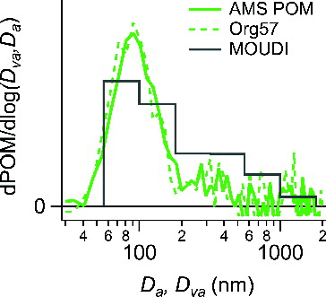
The AMS provides chemically resolved, mass-weighted size distributions according to the vacuum aerodynamic diameter, D_va. Vehicle emissions are characterized by large quantities of small particles in the 30–60 nm (mobility diameter, number-weighted) range (Kittelson et al. 2006) and tend to be fractal-like. As shown in Figure 2, the dominant mass-based size mode of vehicle POM is centered at D_va ∼ 90 nm with some evidence of larger particles at sizes greater than 200 nm. The same pattern is observed for the size distribution for m/z 57 (mostly C₄H₉⁺), which is a marker ion for long chain hydrocarbons. The size distribution of POM derived from the MOUDI (aerodynamic diameter, mass-weighted) is added for comparison and shows consistent results (Figure 2). Note that in a vehicle chase study conducted in New York City in summer 2001, Canagaratna et al. (2004) also observed an ultrafine mode centered at D_va ∼ 90 nm in the mass-based size distribution of fresh vehicle exhaust. In addition, a similar size distribution was observed for the PMF-derived HOA factor in a near-highway sampling experiment (Sun et al. 2011, 2012).

FIG. 2. Average size distributions of POM in LDV emission measured by AMS and MOUDI. The signal at m/z 57, or Org57, is shown as a reference. Size distributions are normalized to have equal areas.

3.3. Variations of POM Composition and Oxidation Degree as a Function of POM Concentration

As discussed in Section 3.1, the gasoline LEV display high variability in POM emissions. The relatively fast sampling time of the AMS during this experiment allows transient behavior of PM composition to be captured. It appears that the overall PM concentration affects the composition of POM. In particular, there is a higher fraction of oxygenated compounds during low concentration periods. In order to investigate this statistically, data across all vehicle tests were lumped into concentration bins. Note that three of the eight vehicles dominate the three largest concentration bins. In Figures 3a–e a statistical analysis is performed on five prominent ions of POM in the AMS spectra. The fraction of these ions with respect to overall organic signal is depicted by box plot analysis and is binned by overall mass concentration. The average mass concentrations for the 0.5–1, 1–2, 2–5, 5–10, 10–15, and >15 μg/m³ bins are 0.71 ± 0.15, 1.4 ± 0.30, 3.0 ± 0.76, 6.9 ± 1.6, 13 ± 1.2, and 18 ± 1.3 μg/m³, respectively. The number of mass spectra in each bin is 160, 99, 40, 22, 9, and 10, respectively. The DL for organics of each concentration bin can be characterized based on scaling the calculated 10-s DL reported Section 2.4 by the square root of the ratio of 10 s to total average time in one bin (i.e., number of data points × 10) (DeCarlo et al. 2006). This yields DLs of 8.4, 11, 17, 23, 35, and 33 ng/m³ for the 0.5–1, 1–2, 2–5, 5–10, 10–15, and >15 μg/m³ size bin, respectively. The average mass spectra of POM corresponding to the different mass concentration bins are shown in Figure S6 and a summary of the main features are shown in Figures 3f–j. The relative importance of primary hydrocarbon ions, e.g., C₄H₇⁺ (m/z = 55) and C₄H₉⁺ (m/z = 57), tends to increase with increased POM concentration. The relative importance of oxygenated ions, e.g., C₂H₃O⁺ (m/z = 43), CO₂⁺ (m/z = 44), and C₂H₄O₂⁺ (m/z = 60), tends to decrease with increasing POM mass. The distribution for the average fraction of particle phase CO₂⁺ (f_CO2) levels out at ∼1% at higher POM concentration (Figure 3e). As a result, the average oxidation degree of POM is anticorrelated with overall POM mass concentration. For example, for POM concentration between 1 and 2 μg/m³, the atomic oxygen-to-carbon ratio, O/C, is 0.088 (Figure 3g) and carbon-containing oxygenated ions (i.e., ΣC_xH_yO_z⁺) together make up 9% of the total POM spectral signal (Figure 3i). For mass bins higher than 2 μg/m³ the O/C decreases, which is reflected by a decreasing contribution of the CO₂⁺ ion and other oxygenated ions and an increase in the contribution of the hydrocarbon ions, C_xH_y⁺. At the highest concentration category hydrocarbon ions make up almost 96% of the POM spectral signal and the O/C is as low as 0.022 (Figure 3g). In order to determine vehicle-to-vehicle variations in POM mass spectra, a mass spectrum from a single concentration bin was derived from each vehicle and correlation analysis was performed on the resulting eight HMR spectra. High correlations (Pearson's r > 0.98) were found, indicating small vehicle-to-vehicle variability. It was thus determined that POM concentration had a greater effect on composition than individual vehicle influences.

FIG. 3. (a–e) Statistical distribution of the fraction of a given ion with respect to overall organic mass plotted as a function of POM concentration using box plots. The crosses represent the mean, the middle bars represent the median, the top and bottom of the box represents the 75th and 25th percentile, respectively, and the top and bottom whiskers represent the 90th and 10th percentile, respectively. (f–j) Summaries of the average H/C, O/C, OM/OC, total signal of oxygenated ions, and f₄₄ of POM as a function of POM concentration. Error bars represent standard error of the mean. For (f–j), a background subtraction has been applied as discussed in Section S2.2 of the online supplementary information.

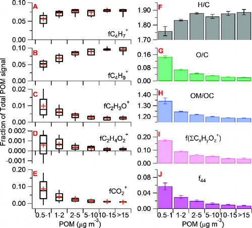
In order to relate these results to AMS measurements made with unit-mass resolution spectrometers, the f₄₄ signal (fraction of all ions at m/z = 44 relative to all POM signals) was compared to the O/C ratios found for each of the mass bins in Figure 3. Figure S7 indicates that a linear relationship exists between O/C and f₄₄ with a best fit of: O/C = 2.5 × f₄₄ − 0.00045.

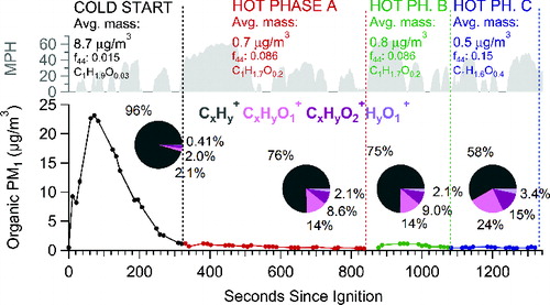
Similar results are obtained when examining the chemical change among UC phases for a single vehicle test (Figure 4). Vehicle 6 was chosen as a test case because it displayed high POM concentration variability (in the range of 0.08–23.3 μg/m³). The emission of less oxidized POM during high mass concentration periods, particularly the cold start, may be attributable to greater influence of lubricating oil compared to combustion-derived products. The influence of lubricating oil on vehicle emissions has been discussed extensively elsewhere (de Albuquerque et al. 2011; Sonntag et al. 2012; Worton et al. 2014). Further evidence can be found by examining the ratio of C₄H₉⁺ (m/z = 57) to C₄H₇⁺ (m/z = 55), which represent saturated (C_nH_2n+1⁺) and unsaturated (C_nH_2n-1⁺) hydrocarbon ion series, respectively. Spectra of lubricating oil tend to display higher m/z57/m/z55 ratios (Canagaratna et al. 2004; Zhang et al. 2005) and Figure S6 shows that as POM concentration increases, this ratio does indeed increase. Since lubricating oil passes through the engine and is exhausted with minimal transformation it retains a majority of the properties of the original lubricating oil and is expected to have low oxygen content. In contrast, some POM from vehicles results from incomplete combustion of fuel, and this combustion-derived POM is likely to be somewhat more oxygenated. As such, it seems plausible that the differences in the O/C (and in particular ions) between the different phases (Figure 4) are a result of a time-varying (phase-dependent) distribution between lubricating oil and combustion-derived POM. The results here suggest a larger fraction of lubricating oil is emitted during the cold-start phase than during other periods, which become increasingly dominated by combustion-derived POM. In this case, the apparent relationship between O/C and POM concentration reflects a correlation between POM concentration and the dominant type of emitted particles. Furthermore, particles emitted during the cold start (highest concentration period) were found to be more volatile than particles emitted in the hot phase (lower concentration periods) (Kuwayama et al. 2014). This behavior is consistent with larger fractions of lubricating oil POM during the higher POM periods of the current study. In addition, it is also possible that the observed O/C versus mass concentration relationship is determined by partitioning of semivolatile species. As the total mass concentration decreases, partitioning theory predicts that compounds with higher vapor pressures will preferentially partition to the gas-phase. To the extent that the less oxygenated components are more volatile than the oxygenated components, a decrease in POM mass should correspond to an increase in POM O/C.

FIG. 4. Comparison of the ion family breakdown for each phase of vehicle 6 test. The traces correspond to the POM concentration for vehicle 6 and are divided into cold start, hot phase A which includes a hard acceleration and sustained high speeds, hot phase B, which includes a second hard acceleration and hot phase C corresponding to the final portion of the hot-phase. The pie charts depict the average contribution of each ion family to the average MS for the given phase. Values in pie may not add up to 100% due to rounding of values to maintain less than 3 significant figures.

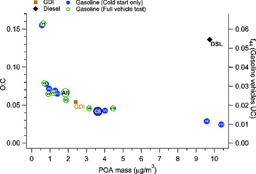
Figures 5a and b shows mass-weighted average HMR spectra for all eight gasoline spark ignition vehicles averaged over the full UC vehicle test and over the cold start periods. Figure 5c and d depicts the average HMR spectra for the GDI and diesel vehicles, respectively. For the alternative vehicles there is also evidence of oxygenated species; for diesel in particular, particle-phase CO₂⁺ appears to be relatively high. A similar ratio between the contribution at m/z = 44 (predominantly CO₂⁺) and total organics was found for diesel exhaust elsewhere (Schneider et al. 2006). The HMR spectrum for ULEV is not shown here primarily due to very low POM concentrations (0.22 μg/m³) similar to background concentrations. In order to summarize these findings the O/C is plotted versus average mass concentration for each individual vehicle where each vehicle has both the cold start and full vehicle test information. Figure 6 shows there is a clear relationship between oxidation degree and POM mass concentration, where higher mass leads to lower O/C, with the exception of the diesel vehicle which had a high O/C of 0.14 coupled with high POM concentration. As discussed above, this relationship may reflect differences in volatility of more versus less oxygenated compounds, or could indicate that the relationship between total POM emitted and the nature of the emitted particles (i.e., lubricating oil versus combustion derived) applies more generally to gasoline vehicles. The O/C for the diesel-derived POM deviates from the O/C curve for gasoline vehicles, suggesting that the diesel vehicle emits less lubricating oil compared to fuel combustion POM. Therefore, the observed O/C depends on the balance between lubricating oil and combustion-derived POM and its relationship to mass concentration appears to vary between spark ignition gasoline and diesel vehicles. The grouping of points approaching O/C ∼0.10 at low POM concentration suggests that the O/C of combustion-derived POM is close to 0.10, while the high POM concentration observations suggest that lubricating oil that is passed through the engine and exhaust system has an O/C of ∼0.025. Note that two gasoline vehicles at low concentrations had higher O/C values of ∼0.16.

FIG. 5. Reference mass spectra of different vehicle POM from this study. In each mass spectrum, the peaks are broken down by ion family and the average elemental ratios are shown in the legend. The pie charts depict the relative contribution of each ion family to the overall mass spectrum. Note that values in pie may not add up to 100% due to rounding of values to maintain less than 3 significant figures.

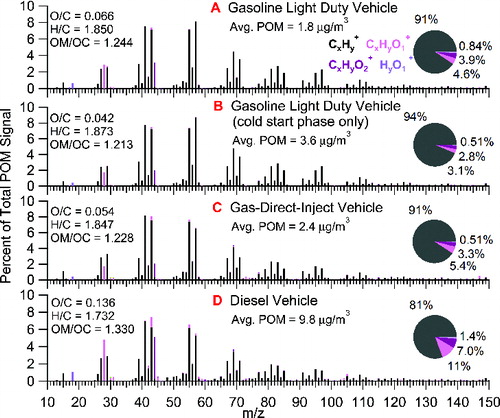
FIG. 6. O/C versus average POM concentration for each vehicle averaged over cold start portion or entire vehicle test for gasoline LEVs. Larger symbols depict average mass spectra from Figure 5. Alternative vehicle mass spectra are depicted by separate symbols. The corresponding f₄₄ values can be traced to right vertical axis for gasoline vehicles where right axis is scaled to left axis according to linear fit derived in Figure S7. The f₄₄ for the diesel vehicle is 0.048 (Figure S7).

3.4. POM Mass Spectral Features and Comparison with Ambient HOA Factors

Figure 5 summarizes the representative HMR spectra of POM from different vehicle types. The most dominant peaks in the spectra are C_xH_y⁺ ions. They exhibit the so-called “picket-fence” fragmentation pattern which is typical of long-chain hydrocarbons (Zhang et al. 2005). The HMR spectra also exhibit oxygenated ion fragments, consistent with other vehicle emission sampling tests which have found strong evidence of light oxygenated compounds in particles (Jakober et al. 2008). Higher order oxygenated ion fragments are also present, the most significant one being CO₂⁺ at m/z = 44. The other major C_xH_yO₂⁺ ion is C₂H₄O₂⁺ at m/z = 60. The diesel vehicle (Figure 5d) displays a high fraction of these oxygenated compounds while having a higher average mass concentration. The GDI vehicle (Figure 5c), on the other hand, has a very similar mass spectrum and oxidation degree as the averaged gasoline vehicles (Figure 5a).

A comparison of the HMR spectra reported in Figure 5 to HOA spectra determined from PMF analysis of ambient particles shows high linear correlations, with Pearson's r value ranging between 0.79 and 0.99. Figures S8–S11 depict a cross-correlation analysis between the mass spectra derived here and those of various ambient and laboratory POM downloaded from http://cires.colorado.edu/jimenez-group/AMSsd/. The ambient studies include HOA spectra from urban sampling sites (Zhang et al. 2005; Lanz et al. 2007a, 2007b; Hersey et al. 2011; Crippa et al. 2013). Additional mass spectra from atomized lubricating oil (Canagaratna et al. 2004) and from the exhaust of a gasoline vehicle (Mohr et al. 2009) have also been considered. The lowest correlation between this study and all other studies was r = 0.79 and was between the diesel test mass spectrum of this study and the HOA factor derived from a study that took place in Zurich in summer (Lanz et al. 2007a). The best correlation was found between the GDI mass spectrum of this study and the HOA factor derived from a study that took place in Paris in winter (Crippa et al. 2013) (r = 0.96). The cold start POM spectrum derived here correlated well with both the lubricating oil spectrum (r = 0.96) and the literature gasoline vehicle (r = 0.95). This suggests that lubricating oil may be an important component of the POM sampled during this study, especially during the cold start. It was also found that the cold start POM spectrum correlated with all other HOA mass spectra to a higher degree than with the full vehicle test mass spectrum. It should be noted that some of the differences between different studies may also reflect differences in the operation of the various AMS instruments.

4. CONCLUSION

A comprehensive vehicle emissions experiment has been carried out using various on-road low-emission vehicles running on a chassis dynamometer. The exhausts of the vehicles were diluted and mixed in a secondary dilution system prior to sampling by various real-time instruments. The dilution was controlled in order to attain atmospherically relevant conditions (0.5–30 μg/m3). In this article the results acquired with an Aerodyne AMS have been thoroughly analyzed. It was found that the cold start portion of the drive cycle had the highest overall emissions for all vehicles. The average mass spectrum of each vehicle was determined and data points from all spark-ignition gasoline vehicles were binned by POM concentration after SDS dilution and an average HMR spectrum was reported for each concentration bin. This was done to investigate trends of all vehicles, rather than focusing on individual vehicles. The average O/C ratios of vehicle POM were low, but were found to be dependent on POM concentration—POM tended to have higher O/C values at lower concentration. This relationship likely arises due to two reasons: (1) partitioning of the more volatile fraction to the gas-phase at lower POM concentration and (2) the composition of the emitted particles (i.e., lubricating oil versus combustion of fuel) is dependent on driving behavior and engine temperature and thus affects POM concentration. It is hypothesized that high POM emission in cold start conditions and during accelerations is associated with a larger fraction of lubricating oil (less oxidized) in the emissions whereas the POM is composed of a larger fraction of more oxidized fuel combustion PM at lower concentration. Diesel POM was found to be significantly more oxidized than gasoline POM at the same POM concentration, pointing to an important difference in chemistry between the two vehicle types.

A comparison with ambient derived HOA factors demonstrated a high correlation between tail-pipe vehicle emissions and these ambient factors. A mass spectrum from atomized lubricating oil and tail-pipe emissions from a separate study were also included in the comparison. It was found that the unit mass resolution spectrum of the averaged cold start tests (Figure 5b) had a higher correlation with the literature HOA factors as compared to that of the full vehicle test mass spectrum (Figure 5a). This is an indication that cold-start has an important effect on the characteristics of vehicle POM. In particular, the cold-start condition appears to emit particles that have chemical composition more closely resembling the ambient HOA factors as well as that of the atomized lubricating oil. In the hot-phase, the aerosol from vehicle tail-pipe emissions tends to be more oxidized and their AMS spectra show a more dominant particle phase CO₂⁺ peak. Statistically meaningful trends of oxidation degree were observed as a function of overall concentration, which points to dynamic partitioning behavior and may also reflect importance of driving conditions and contribution from lubricating oil. Furthermore, the mass spectra reported here can be used as reference spectra for on-road vehicle emissions, while also demonstrating that these spectra may be dependent on loading. Since ambient HOA loading can vary widely (Zhang et al. 2007; Ng et al. 2010), this conclusion has important implications for interpretation of HOA-like factors derived from ambient measurements.

SUPPLEMENTAL MATERIAL

Supplemental data for this article can be accessed on the publisher's website.

ACKNOWLEDGMENTS

The authors thank Professor Kyaw Tha Paw U (UCD) for lending them the LI-COR CO₂ analyzer and the engineers at the Haagen-Smit Vehicle Testing Facility for assisting during the dynamometer experiments.

Funding

This work was partially funded by U.S. Department of Energy (DOE), Atmospheric System Research Program, Grant No. DE-FG02-11ER65293. The acquisition of the vehicle emission data was supported by the California Air Resources Board, Research Division under contract #10-313.

REFERENCES

- Alfarra, M. R., Prevot, A. S. H., Szidat, S., Sandradewi, J., Weimer, S., Lanz, V. A., Schreiber, D., Mohr, M., and Baltensperger, U. (2007). Identification of the Mass Spectral Signature of Organic Aerosols from Wood Burning Emissions. Environ. Sci. Technol., 41:5770–5777, doi:10.1021/es062289b.
- Allan, J. D., Alice E. Delia, Huge Coe, Keith N. Bower, M. Rami Alfarra, Jose L. Jimenez, Ann M. Middlebrook, Frank Drewnick, Timothy B. Onasch, Manjula R. Canagaratna, John T. Jayne, and Worsnop, D. R. (2004). Technical Note: A Generalised Method for the Extraction of Chemically Resolved Mass Spectra from Aerodyne Aerosol Mass Spectrometer Data. J. Aerosol. Sci., 35:909–922, doi:10.1016/j.jaerosci.2004.02.007.
- Austin, T. C., DeGenova, F. J., Caelson, T. R., Joy, R. W., and Gianolini, K. A. (1993). Characterization of Driving Patterns and Emissions from Light-Duty Vehicles in California. No. ARB-R-949-508.
- Ban-Weiss, G. A., Lunden, M. M., Kirchstetter, T. W., and Harley, R. A. (2010). Size-Resolved Particle Number and Volume Emission Factors for On-Road Gasoline and Diesel Motor Vehicles. J. Aerosol. Sci., 41:5–12, doi:10.1016/j.jaerosci.2009.08.001.
- Baynard, T., Lovejoy, E. R., Pettersson, A., Brown, S. S., Lack, D., Osthoff, H., Massoli, P., Ciciora, S., Dube, W. P., and Ravishankara, A. R. (2007). Design and Application of a Pulsed Cavity Ring-Down Aerosol Extinction Spectrometer for Field Measurements. Aerosol Sci. Technol., 41:L447–462, doi:10.1080/02786820701222801.
- Beddows, D. C. S., and Harrison, R. M. (2008). Comparison of Average Particle Number Emission Factors for Heavy and Light Duty Vehicles Derived from Rolling Chassis Dynamometer and Field Studies. Atmos. Environ., 42:7954–7966, doi:10.1016/j.atmosenv.2008.06.021.
- Canagaratna, M. R., Jayne, J. T., Ghertner, D. A., Herndon, S., Shi, Q., Jimenez, J. L., Silva, P. J., Williams, P., Lanni, T., Drewnick, F., Demerjian, K. L., Kolb, C. E., and Worsnop, D. R. (2004). Chase Studies of Particulate Emissions from in-use New York City Vehicles. Aerosol Sci. Technol., 38:555–573, doi:10.1080/02786820490465504.
- Canagaratna, M. R., Onasch, T. B., Wood, E. C., Herndon, S. C., Jayne, J. T., Cross, E. S., Miake-Lye, R. C., Kolb, C. E., and Worsnop, D. R. (2010). Evolution of Vehicle Exhaust Particles in the Atmosphere. J. Air Waste Manage. Assoc., 60:1192–1203, doi:10.3155/1047-3289.60.10.1192.
- Collier, S., and Zhang, Q. (2013). Gas-Phase CO2 Subtraction for Improved Measurements of the Organic Aerosol Mass Concentration and Oxidation Degree by an Aerosol Mass Spectrometer. Environ. Sci. Technol., 47:14324–14331, doi:10.1021/es404024h.
- Crippa, M., DeCarlo, P. F., Slowik, J. G., Mohr, C., Heringa, M. F., Chirico, R., Poulain, L., Freutel, F., Sciare, J., Cozic, J., Di Marco, C. F., Elsasser, M., Nicolas, J. B., Marchand, N., Abidi, E., Wiedensohler, A., Drewnick, F., Schneider, J., Borrmann, S., Nemitz, E., Zimmermann, R., Jaffrezo, J. L., Prévôt, A. S. H., and Baltensperger, U. (2013). Wintertime Aerosol Chemical Composition and Source Apportionment of the Organic Fraction in the Metropolitan Area of Paris. Atmos. Chem. Phys., 13:961–981, doi:10.5194/acp-13-961-2013.
- de Albuquerque, P. C. C., de Andrade Ávila, R. N., Barros Zárante, P. H., and Sodré, J. R. (2011). Lubricating Oil Influence on Exhaust Hydrocarbon Emissions from a Gasoline Fueled Engine. Tribol. Int., 44:1796–1799.
- DeCarlo, P. F., Kimmel, J. R., Trimborn, A., Northway, M. J., Jayne, J. T., Aiken, A. C., Gonin, M., Fuhrer, K., Horvath, T., Docherty, K. S., Worsnop, D. R., and Jimenez, J. L. (2006). Field-Deployable, High-Resolution, Time-of-Flight Aerosol Mass Spectrometer. Anal. Chem., 78:8281–8289, doi:10.1021/ac061249n.
- Forestieri, S., Collier, S., Kuwayama, T., Zhang, Q., Kleeman, M. J., and Cappa, C. D. (2013). Real-Time Black Carbon Emission Factor Measurements from Light Duty Vehicles. Environ. Sci. Technol., 47:13104–13112, doi:10.1021/es401415a.
- Grieshop, A. P., Lipsky, E. M., Pekney, N. J., Takahama, S., and Robinson, A. L. (2006). Fine Particle Emission Factors from Vehicles in a Highway Tunnel: Effects of Fleet Composition and Season. Atmos. Environ., 40(2):287–298.
- Gross, D. S., Barron, A. R., Sukovich, E. M., Warren, B. S., Jarvis, J. C., Suess, D. T., and Prather, K. A. (2005). Stability of Single Particle Tracers for Differentiating Between Heavy- and Light-Duty Vehicle Emissions. Atmos. Environ., 39:2889–2901, doi:10.1016/j.atmosenv.2004.12.044.
- Hasheminassab, S., Daher, N., Schauer, J. J., and Sioutas, C. (2013). Source Apportionment and Organic Compound Characterization of Ambient Ultrafine Particulate Matter (pm) in the Los Angeles Basin. Atmos. Environ., 79:529–539.
- He, L. Y., Lin, Y., Huang, X. F., Guo, S., Xue, L., Su, Q., Hu, M., Luan, S. J., and Zhang, Y. (2010). Characterization of High-Resolution Aerosol Mass Spectra of Primary Organic Aerosol Emissions from Chinese Cooking and Biomass Burning. Atmos. Chem. Phys., 10:11535–11543, doi:10.5194/acp-10-11535-2010.
- Herndon, S. C., Onasch, T. B., Wood, E. C., Kroll, J. H., Canagaratna, M. R., Jayne, J. T., Zavala, M. A., Knighton, W. B., Mazzoleni, C., Dubey, M. K., Ulbrich, I. M., Jimenez, J. L., Seila, R., Gouw, J. A. d., Foy, B. d., Fast, J., Molina, L. T., Kolb, C. E., and Worsnop, D. R. (2008). The Correlation of Secondary Organic Aerosol with Odd Oxygen in Mexico City. Geophys. Res. Lett., 35:L15804, doi:10.1029/2008GL034058.
- Hersey, S. P., Craven, J. S., Schilling, K. A., Metcalf, A. R., Sorooshian, A., Chan, M. N., Flagan, R. C., and Seinfeld, J. H. (2011). The Pasadena Aerosol Characterization Observatory (paco): Chemical and Physical Analysis of the Western Los Angeles Basin Aerosol. Atmos. Chem. Phys., 11:7417–7443, doi:10.5194/acp-11-7417-2011.
- Jakober, C. A. M. A. R., Riddle, S. G., Destaillats, H., Charles, M. J., Green, P. G., and Kleeman, M. J. (2008). Carbonyl Emissions from Gasoline and Diesel Motor Vehicles. Environ. Sci. Technol., 42:4697–4703.
- Jimenez, J. L., Jayne, J. T., Shi, Q., Kolb, C. E., Worsnop, D. R., Yourshaw, I., Seinfeld, J. H., Flagan, R. C., Zhang, X., Smith, K. A., Morris, J. W., and Davidovits, P. (2003). Ambient Aerosol Sampling using the Aerodyne Aerosol Mass Spectrometer. J. Geophys. Res.: Atmos., 108:8425, doi:10.1029/2001JD001213.
- Jimenez, J. L., Canagaratna, M. R., Donahue, N. M., Prevot, A. S. H., Zhang, Q., Kroll, J. H., DeCarlo, P. F., Allan, J. D., Coe, H., Ng, N. L., Aiken, A. C., Docherty, K. S., Ulbrich, I. M., Grieshop, A. P., Robinson, A. L., Duplissy, J., Smith, J. D., Wilson, K. R., Lanz, V. A., Hueglin, C., Sun, Y. L., Tian, J., Laaksonen, A., Raatikainen, T., Rautiainen, J., Vaattovaara, P., Ehn, M., Kulmala, M., Tomlinson, J. M., Collins, D. R., Cubison, M. J., E., Dunlea, J., Huffman, J. A., Onasch, T. B., Alfarra, M. R., Williams, P. I., Bower, K., Kondo, Y., Schneider, J., Drewnick, F., Borrmann, S., Weimer, S., Demerjian, K., Salcedo, D., Cottrell, L., Griffin, R., Takami, A., Miyoshi, T., Hatakeyama, S., Shimono, A., Sun, J. Y., Zhang, Y. M., Dzepina, K., Kimmel, J. R., Sueper, D., Jayne, J. T., Herndon, S. C., Trimborn, A. M., Williams, L. R., Wood, E. C., Middlebrook, A. M., Kolb, C. E., Baltensperger, U., and Worsnop, D. R. (2009). Evolution of Organic Aerosols in the Atmosphere. Science, 326:1525–1529, doi:10.1126/science.1180353.
- Kittelson, D. B., Watts, W. F., Johnson, J. P., Schauer, J. J., and Lawson, D. R. (2006). On-Road and Laboratory Evaluation of Combustion Aerosols—Part 2: Summary of Spark Ignition Engine Results. J. Aerosol. Sci., 37:931–949, doi:10.1016/j.jaerosci.2005.08.008.
- Kuwayama, T., Collier, S., Forestieri, S., Brady, J. M., Bertram, T. H., Cappa, C. D., Zhang, Q., and Kleeman, M. J. (2014). Volatility of Primary Organic Aerosol Emitted from Light Duty Gasoline Vehicles. Environ. Sci. Technol., DOI: 10.1021/es504009w.
- Lack, D., Lovejoy, E. R., Baynard, T., Pettersson, A., and Ravishankara, A. R. (2006). Aerosol Absorption Measurement using Photoacoustic Spectroscopy: Sensitivity, Calibration, and Uncertainty Developments. Aerosol Sci. Technol., 40:697–708, doi:10.1080/02786820600803917.
- Lanz, V. A., Alfarra, M. R., Baltensperger, U., Buchmann, B., Hueglin, C., and Prévôt, A. S. H. (2007a). Source Apportionment of Submicron Organic Aerosols at an Urban Site by Factor Analytical Modelling of Aerosol Mass Spectra. Atmos. Chem. Phys., 7:1503–1522, doi:10.5194/acp-7-1503-2007.
- Lanz, V. A., lfarra, M. R., Baltensperger, U., Buchmann, B., Hueglin, C., Szidat, S., Wehrli, M. N., Wacker, L., Weimer, S., Caseiro, A., Puxbaum, H., and Prevot, A. S. H. (2007b). Source Attribution of Submicron Organic Aerosols During Wintertime Inversions by Advanced Factor Analysis of Aerosol Mass Spectra. Environ. Sci. Technol., 42:214–220, doi:10.1021/es0707207.
- Massoli, P., Fortner, E. C., Canagaratna, M. R., Williams, L. R., Zhang, Q., Sun, Y., Schwab, J. J., Trimborn, A., Onasch, T. B., Demerjian, K. L., Kolb, C. E., Worsnop, D. R., and Jayne, J. T. (2012). Pollution Gradients and Chemical Characterization of Particulate Matter from Vehicular Traffic Near Major Roadways: Results from the 2009 Queens College Air Quality Study in NYC. Aerosol Sci. Tech., 46:1201–1218, doi:10.1080/02786826.2012.701784.
- Middlebrook, A. M., Bahreini, R., Jimenez, J. L., and Canagaratna, M. R. (2012). Evaluation of Composition-Dependent Collection Efficiencies for the Aerodyne Aerosol Mass Spectrometer using Field Data. Aerosol Sci. Technol., 46:258–271, doi:10.1080/02786826.2011.620041.
- Mohr, C., Huffman, J. A., Cubison, M. J., Aiken, A. C., Docherty, K. S., Kimmel, J. R., Ulbrich, I. M., Hannigan, M., and Jimenez, J. L. (2009). Characterization of Primary Organic Aerosol Emissions from Meat Cooking, Trash Burning, and Motor Vehicles with High-Resolution Aerosol Mass Spectrometry and Comparison with Ambient and Chamber Observations. Environ. Sci. Technol., 43:2443–2449, doi:10.1021/es8011518.
- Ng, N. L., Canagaratna, M. R., Zhang, Q., Jimenez, J. L., Tian, J., Ulbrich, I. M., Kroll, J. H., Docherty, K., Chhabra, P. S., Bahreini, R., Murphy, S. M., Seinfeld, J. H., Hildebrandt, L., Donahue, N. M., DeCarlo, P. F., Lanz, V. A., Prévôt, A. S. H., Dinar, E., Rudich, Y., and Worsnop, D. R. (2010). Organic Aerosol Components Observed in Northern Hemispheric Datasets from Aerosol Mass Spectrometry. Atmos. Chem. Phys., 10:4625–4641.
- Paatero, P., and Tapper, U. (1994). Positive Matrix Factorization: A Non-Negative Factor Model with Optimal Utilization of Error Estimates of Data Values. Environmetrics, 5:111–126, doi:10.1002/env.3170050203.
- Pant, P., and Harrison, R. M. (2013). Estimation of the Contribution of Road Traffic Emissions to Particulate Matter Concentrations from Field Measurements: A Review. Atmos. Environ., 77:78–97.
- Pierson, W. R., Gertler, A. W., Robinson, N. F., Sagebiel, J. C., Zielinska, B., Bishop, G. A., Stedman, D. H., Zweidinger, R. B., and Ray, W. D. (1996). Real-World Automotive Emissions—Summary of Studies in the Fort Mchenry and Tuscarora Mountain Tunnels. Atmos. Environ., 30:2233–2256, doi:10.1016/1352-2310(95)00276-6.
- Robert, M. A., VanBergen, S., Kleeman, M. J., and Jakober, C. A. (2007). Size and Composition Distributions of Particulate Matter Emissions: Part 1—Light-Duty Gasoline Vehicles. J. Air Waste Manage. Assoc., 57:1414–1428, doi:10.3155/1047-3289.57.12.1414.
- Schauer, J. J., Rogge, W. F., Hildemann, L. M., Mazurek, M. A., and Cass, G. R. (1996). Source Apportionment of Airborne Particulate Matter using Organic Compounds as Tracers. Atmos. Environ., 30:3837–3855.
- Schauer, J. J., Christensen, C. G., Kittelson, D. B., Johnson, J. P., and Watts, W. F. (2008). Impact of Ambient Temperatures and Driving Conditions on the Chemical Composition of Particulate Matter Emissions from Non-Smoking Gasoline-Powered Motor Vehicles. Aerosol Sci. Technol., 42:210–223, doi:10.1080/02786820801958742.
- Schneider, J., Weimer, S., Drewnick, F., Borrmann, S., Helas, G., Gwaze, P., Schmid, O., Andreae, M. O., and Kirchner, U. (2006). Mass Spectrometric Analysis and Aerodynamic Properties of Various Types of Combustion-Related Aerosol Particles. Int. J. Mass Spectromet., 258:37–49, doi:10.1016/j.ijms.2006.07.008.
- Sonntag, D. B., Bailey, C. R., Fulper, C. R., and Baldauf, R. W. (2012). Contribution of Lubricating Oil to Particulate Matter Emissions from Light-Duty Gasoline Vehicles in Kansas City. Environ. Sci. Technol., 46:4191–4199, doi:10.1021/es203747f.
- Sun, Y.-L., Zhang, Q., Schwab, J. J., Demerjian, K. L., Chen, W.-N., Bae, M.-S., Hung, H.-M., Hogrefe, O., Frank, B., Rattigan, O. V., and Lin, Y.-C. (2011). Characterization of the Sources and Processes of Organic and Inorganic Aerosols in New York City with a High-Resolution Time-of-Flight Aerosol Mass Apectrometer. Atmos. Chem. Phys., 11:1581–1602, doi:10.5194/acp-11-1581-2011.
- Sun, Y. L., Zhang, Q., Schwab, J. J., Chen, W.-N., Bae, M.-S., Hung, H.-M., Lin, Y.-C., Ng, N. L., Jayne, J., Massoli, P., Williams, L. R., and Demerjian, K. L. (2012). Characterization of Near-Highway Submicron Aerosols in New York City with a High-Resolution Time-of-Flight Aerosol Mass Spectrometer. Atmos. Chem. Phys., 12:2215–2227, doi:10.5194/acp-12-2215-2012.
- Watson, J. G., Zhu, T., Chow, J. C., Engelbrecht, J., Fujita, E. M., and Wilson, W. E. (2002). Receptor Modeling Application Framework for Particle Source Apportionment. Chemosphere, 49:1093–1136.
- Worton, D. R., Isaacman, G., Gentner, D. R., Dallmann, T. R., Chan, A. W. H., Ruehl, C. R., Kirchstetter, T., Wilson, K. R., Harley, R. A., and Goldstein, A. H. (2014). Lubricating Oil Dominates Primary Organic Aerosol Emissions from Motor Vehicles. Environ. Sci. Technol., 48:3698–3706, doi:10.1021/es405375j.
- Zhang, Q., Alfarra, M. R., Worsnop, D. R., Allan, J. D., Coe, H., Canagaratna, M. R., and Jimenez, J. L. (2005). Deconvolution and Quantification of Hydrocarbon-Like and Oxygenated Organic Aerosols Based on Aerosol Mass Spectrometry. Environ. Sci. Technol., 39:4938–4952.
- Zhang, Q., Jimenez, J. L., Canagaratna, M. R., Allan, J. D., Coe, H., Ulbrich, I., Alfarra, M. R., Takami, A., Middlebrook, A. M., Sun, Y. L., Dzepina, K., Dunlea, E., Docherty, K., DeCarlo, P. F., Salcedo, D., Onasch, T., Jayne, J. T., Miyoshi, T., Shimono, A., Hatakeyama, S., Takegawa, N., Kondo, Y., Schneider, J., Drewnick, F., Borrmann, S., Weimer, S., Demerjian, K., Williams, P., Bower, K., Bahreini, R., Cottrell, L., Griffin, R. J., Rautiainen, J., Sun, J. Y., Zhang, Y. M., and Worsnop, D. R. (2007). Ubiquity and Dominance of Oxygenated Species in Organic Aerosols in Anthropogenically-Influenced Northern Hemisphere Midlatitudes. Geophys. Res. Lett., 34:L13801, doi:10.1029/2007GL029979.
- Zhang, Q., Jimenez, J. L., Canagaratna, M. R., Ulbrich, I. M., Ng, N. L., Worsnop, D. R., and Sun, Y. (2011). Understanding Atmospheric Organic Aerosols via Factor Analysis of Aerosol Mass Spectrometry: A Review. Anal. Bioanal. Chem., 401:3045–3067, doi:10.1007/s00216-011-5355-y.