An Analytic Equation for the Volume Fraction of Condensationally Grown Mixed Particles and Applications to Secondary Organic Material Produced in Continuously Mixed Flow Reactors

Abstract

Secondary condensation of organic material onto primary seed particles is one pathway of particle growth in the atmosphere, and many properties of the resulting mixed particles depend on organic volume fraction. Environmental chambers can be used to simulate the production of these types of particles, and the optical, hygroscopic, and other properties of the mixed particles can be studied. In the interpretation of the measured properties, the probability density function p(ϵ;d) of volume fraction ϵ of the condensing material for particle diameter d in the outflow of the chamber is typically needed. In this article, analytic equations are derived p(ϵ;d) for condensational growth in a continuously mixed flow reactor. The equation predictions are compared to measurements for the condensation of secondary organic material on quasi-monodisperse sulfate seed particles. Equations are presented herein for discrete, Gaussian, and triangular distribution functions for the seed particle number–diameter distributions, including generalization to any linearly segmented distributions. The analytic equations are useful both for the interpretation of laboratory data from environmental chambers, such as the construction of probability density functions for use in interpretation of hygroscopic growth data, cloud–condensation–nuclei data, or other laboratory data sets dependent on organic volume fraction, as well as for understanding atmospheric processes at times that condensational growth processes prevail.

Copyright 2014 American Association for Aerosol Research

1. INTRODUCTION

Atmospheric particles have significant effects on air quality and climate, and an important source of particulate material is the production of secondary organic material (Seinfeld and Pandis 2006). A common atmospheric particle type observed by microscopy consists of a primary particle coated by secondary organic material (Pöschl et al. 2010). Secondary organic material is produced by multiple pathways (Hallquist et al. 2009), and for certain reaction conditions condensational growth can be the dominant pathway (Seinfeld et al. 2003; Kuwata and Martin 2012). The production pathways of secondary organic material have been widely simulated in laboratory environmental chambers in efforts to understand and quantify the involved chemistry and associated environmental effects (Hallquist et al. 2009). One common configuration is to operate the chamber as a continuously mixed flow reactor (CMFR; Kleindienst et al. 1999; Shilling et al. 2008; King et al. 2009; Mentel et al. 2009; Drozd et al. 2013). The CMFR can be maintained at steady state for weeks at a time, allowing long times for signal integration for online measurements (Shilling et al. 2008) or for sufficient sample collection for offline analysis (You et al. 2012; Renbaum-Wolff et al. 2013; Shrestha et al. 2013). Inorganic seed particles are typically used to suppress oscillatory behavior in the chamber (McGraw and Saunders 1984) and/or to simulate internally mixed atmospheric particles (Seinfeld and Pandis 2006). As a result, mixed inorganic–organic particle populations, similar in microscopy images to those observed for collected atmospheric particles, are produced. In the interpretation of the measured properties, the probability density function p(ϵ;d) of volume fraction ϵ of the condensing material for particle diameter d in the outflow of the chamber is typically needed.

For mixed inorganic–organic particle populations produced by condensational growth in a CMFR, particles of a single diameter d in the CMFR outflow have an associated probability density function p(ϵ) of organic volume fraction ϵ arising from a distribution of individual particle residence times in the CMFR (Davis and Davis 2003). For instance, particles grown on smaller seeds but having longer residence times can have the same final diameter in the CMFR outflow as particles grown on larger seeds but having shorter residence time. Knowledge of p(ϵ) at a specific diameter in the CMFR outflow is important because a size slice of the outflow aerosol is often selected for investigation of additional particle properties, such as hygroscopic growth (Swietlicki et al. 2008), phase transitions (Smith et al. 2011, 2012, 2013), or cloud activation potential (King et al. 2009, 2010). Interpretation of those data sets requires knowledge of p(ϵ) at the analyzed diameter.

TABLE 1. Equations for the distribution functions f(d,t), f(d,d₀), f(d₀,t), f(d,ϵ), and f(d,z)

Symbol	Quantity	Units	CMFR	Restriction	Equation
f(d,t)		m^−3 m^−1 s^−1		x ⩾ 0	(7)
f(d,d0)		m^−3 m^−1 m^−1		d ⩾ d0	(S2)
f(d0,t)		m^−3 m^−1 s^−1		none	(S3)
f(d,ϵ)		m^−3 m^−1		none	(8)
f(d,z)		m^−3 m^−1		none	(9)

In previous treatments, p(ϵ) was simulated numerically by a sectional model (King et al. 2009, 2010; Smith et al. 2011, 2012, 2013). Herein, we develop an analytical expression for p(ϵ) in the outflow from a CMFR. The developed expression is more concise and accurate than the previously used sectional models. The equations are useful both for the interpretation of laboratory data from environmental chambers and for understanding atmospheric processes at times that condensational growth processes prevail.

2 THEORY

2.1 Definition

The theoretical development considers a particle population that begins as monodisperse seed particles of diameter d₀ of a first material upon which a second material condenses to a variable extent on each seed particle (e.g., because of variable exposure times for different seed particles). For an individual particle of diameter d in the population, the volume fraction ϵ(d,d₀) of the second material is given by the following equation: [1]

Both the initial seed particle and the grown particle are taken as effectively spherical. Equation (1)[1] implies that the volume fraction of a growing particle rapidly converges on unity irrespective of the initial seed diameter (e.g., ϵ = 0.98 for d/d₀ = 3.68) (Figure S1). An additional term z, which is the inverse of the diameter growth factor, is useful in presenting succinct equations and is given as follows: [2] The following useful derivative is obtained: [3]

2.2 Definitions f(d,t), f(d,d₀), f(d₀,t), f(d,ϵ), and f(d,z) and Relationships to N, n(d), and p(ϵ)

The particle population in the reactor outflow has a total number concentration N. There are distribution functions f(d,t), f(d,d₀), f(d₀,t), f(d,ϵ), and f(d,z) of the number count of the particle population with respect to particle diameter d, particle residence time t, seed particle diameter d₀, volume fraction ϵ of the second material, and inverse diameter growth factor z (Table 1). The relationship of these distribution functions to the number–diameter distribution n(d) in the reactor outflow is as follows: [4] The distribution n(d) cannot be obtained directly from f(d₀,t) and instead requires a path integral along d through f(d₀,t) (i.e., Equation (6)[6] as one possible example) or a transformation of variables (i.e., thereby recovering one of the forms of Equation (4)[4] ). The total particle number concentration N is given by N = ∫^∞₀n(d) dd.

The probability density function p of volume fraction ϵ for particle diameter d, abbreviated as p(ϵ) or written in full form as p(ϵ;d), is given by the following equation: [5] for which n(d) serves as the normalization term of f(d,ϵ) such that the integral across p(ϵ) is unity. The foregoing equation, as well as several others noted below, is derived in the Supplemental Information. The objective of this study is to provide analytic formulations for p(ϵ), implying by Equation (5)[5] that analytic formulations are also needed for f(d,ϵ) and n(d).

2.3 Condensational Growth Rate

The main application considered in the present study is diameter growth by condensation of organic molecules from the gas phase onto the surfaces of sulfate seed particles. Mixed organic-sulfate particles are the most prevalent submicron particle in anthropogenically affected continental regions of the world (Zhang et al. 2007). For this application, the term ϵ corresponds to the organic volume fraction.

As described in Seinfeld et al. (2003) and Kuwata and Martin (2012), the condensational diameter growth rate I(d), describing dd/dt, is assumed to be adequately described by I(d) = β/(d + λ). Terms include a mean free path λ for the condensing species and a gas-phase concentration parameter β that is proportional to the difference between partial pressure and vapor pressure of the condensing species. Additional considerations related to the physical interpretation of terms λ and β are discussed in Seinfeld et al. (2003) and Kuwata and Martin (2012). These studies have shown that even with the myriad compounds of secondary organic aerosol, the number–diameter distributions of actual data sets, such as those of α-pinene or β-caryophyllene ozonolysis, are adequately represented by I(d) = β/(d + λ). The main intellectual justification for this success is limited variability of mean free paths among different organic molecules.

Integration of the equation for I(d) results in a relationship by which knowledge of any two of d, d₀, and t is sufficient to obtain the third, as follows: [6] This equation defines implicit functions for d(t,d₀) and d₀(d,t) and an explicit function for t(d,d₀). Parameters λ and β are taken as known. In this case, by Equation (6)[6] any two of d, d₀, and t are sufficient to find the third. Furthermore, for fixed β and λ the equation implies that d(t) for different initial diameters constitute a set of non-intersecting lines. Equation (6)[6] omits any treatment of size-dependent behavior, such as by the Kelvin effect.

2.4 Continuously Mixed Flow Reactor

For the case under consideration in this study, the number–diameter distribution n*₀(d) of the seed particles in the inflow to the CMFR is measured or otherwise known. The term n₀(d) describes the seed particle number–diameter distribution in the outflow from the reactor and differs from n*₀(d) because of particle wall loss. The term n(d) describes the number–diameter distribution in the CMFR outflow (i.e., after condensational growth on the seed particles). Coagulation processes affecting n(d) and n₀(d) are not included in the present analysis because for typical environmental chambers they are important only for high number concentrations (>10¹⁰ m³). The possibility of new particle formation is also not included in the model because for typical environmental chambers nucleation is not observed in the presence of seed particles. Possible competing losses of gas-phase species to chamber walls or other surfaces is not relevant in the present treatment because the growth rate law I(d) underlying Equation (6)[6] is prescribed.

Condensational growth occurs onto the seed particles during their distribution of residence times t in the CMFR. The distribution of residence times in a CMFR is described by Poisson statistics. There is a mean reactor residence time τ of the particle population, including loss both by outflow from the CMFR and by deposition on the reactor walls. Particle diameter increases by condensational growth that takes place in the reactor. The distribution of residence times in the CMFR implies a distribution of particle diameters in the reactor outflow.

For the stated conditions and assumptions, the distribution function f(d,t) in the reactor outflow is bivariate in particle diameter d and particle residence time t. It is written as follows for the growth rate law of Equation (6)[6] , as follows (see the online supplemental information [SI]): [7] for . For orientation to the reader, Figure 1a shows an example of a density plot of f(d,t). Figures 1b and c show cross-sections in constant diameter and constant residence time, respectively, through the density plot. Plots for f(d,d₀) and f(d₀,t) are shown in Figures S2 and S3, respectively.

FIG. 1. Distribution function f(d,t). (a) Density plot of f(d,t) as a function of grown particle diameter d and particle residence time t (Equation (7)[7] ). Parameter values τ, β, λ, and n₀(d) are as follows: 10,000 s, 10 nm² s⁻¹, 100 nm, and ∧(10–90 nm) with N_T = 1 m⁻³, respectively. Contours of constant organic volume fraction are shown. The line with arrow shows the forward trajectory of 50-nm seed particles through time. (b) Cross-sections through f(d,t) for fixed d and variable t. The sections are shown for five diameters ranging from 50 to 450 nm. The dashed line in this and other figures is always associated in some manner with 50 nm, which is the mode diameter of the seed particles: n₀(d) = ∧(10–90 nm). (c) Cross-sections through f(d,t) for fixed t and variable d. The sections are shown for nine particle residence times ranging from 0(×10³) to 16(×10³) s. In this panel, the line for t = 0 showing ∧(10–90 nm) represents n₀(d) / τ.

After a transformation of variables, functions f(d, ϵ) and f(d, z) are obtained (see the SI): [8] [9] These expressions, as well as f(d,d₀) and f(d₀,t), are summarized in Table 1. Figure 2 shows density plots of Equation (8)[8] scaled linearly (Figure 2a) as well as logarithmically (Figure 2d). Cross-sections through the density plot are shown in Figures 2b and c. Panels e and f of the figure show probability density functions of organic volume fraction for several different diameter cross-sections (Section 2.5).

The probability density function p(ϵ) at a diameter d is obtained by combining Equations (4), (5), and (9), as follows (see the SI): [10] for the cumulative distribution function c(ϵ;d). The dependence z(ϵ) is given by Equation (2)[2] .

FIG. 2. Distribution function f(d,ϵ). (a) Density plot of f(d,ϵ) as a function of grown particle diameter d and for organic volume fractions ϵ of up to 0.9 (Equation (8)[8] ). Parameter values are as for Figure 1. Contours of constant particle residence time ranging from 2(×10²) to 20(×10²) s are shown. (b) Cross-sections through f(d,ϵ) for fixed d and variable ϵ. The sections are shown for four diameters ranging from 50 to 125 nm. (c) Cross-sections through f(d,ϵ) for fixed ϵ and variable d. The sections are shown for five organic volume fractions ranging from 0.0 to 0.8. (d) Density plot of log₁₀ f(d,ϵ) for organic volume fractions approaching close to unity. Contours of constant particle residence time ranging from 125 to 8000 s are shown. (e) Probability density function p(ϵ;d) of organic volume fraction ϵ for fixed particle diameter d (Equation (5)[5] ). This panel shows p(ϵ;d) for four smaller values of d, ranging from 50 to 125 nm. (f) Same as panel (e) but for five larger values of d, ranging from 50 to 250 nm.

As a reference point, in the limiting case of a monodisperse seed particle population of number concentration N with a distribution defined by a Dirac delta function centered at d₀ (i.e., n₀(d) = N δ(d − d₀)), Equation (10)[10] evaluates to the following (see the SI): [11]

2.5 p() for Discretized n₀(d)

A number–diameter distribution n₀(d) for the seed particles can be discretized into k monodisperse bins of monotonically increasing diameters {d_0,1, d_0,2, …, d_0,k} having respective number concentrations {N₁, N₂, … N_k}. The relationship holds that N = Σ_jN_j for j = [1,k]. Each bin corresponds to a Dirac delta function centered at d_0,j (i.e., n_0,j(d) = N_j δ(d − d_0,j)) and makes a partial contribution to n₀(d) as n₀(d) = Σ_j n_0,j(d) for j = [1,k]. For this case, Equation (10)[10] develops as follows (see the SI): [12]

The index q in the last line for the denominator corresponds to the index of the last element of {d_0,1, d_0,2, …, d_0,k} that satisfies d − d_{0, j} > 0.

The cumulative distribution function c(ϵ) is then given as follows (see the SI): [13] in which r is the index of the first element of {d_0,1, d_0,2, …, d_0,k} that satisfies zd − d_{0, j} < 0.

2.6 p() for Continuous n₀(d)

2.6.1 Gaussian Distribution

For many CMFRs, prior to entering the chamber polydisperse seed particles are classified in unipolar electric mobility by passage through a differential mobility analyzer (DMA) (Knutson and Whitby 1975). A distribution of organic volume fractions arises because of a combination of factors, including Poisson statistics that regulate the residence times of individual particles, the finite width of the DMA transfer function, and the multimodes of seed particles in diameter space (i.e., +1, +2, +3 charges). In diameter space, each charge q contributes one mode to the seed particle population. The mode can be approximately described by a Gaussian distribution characterized by a mode diameter , a variance σ²_q, and a concentration N_q. The associated equation for n₀(d) is as follows: [14]

Although the upper limit of Equation (14)[14] is represented as infinity for completeness, in practice |q| ∈ { + 1, +2, +3} is sufficient. By Equation (10)[10] , the following expression is obtained for p(ϵ;d) (see the SI): [15] for a normalization factor ξ given by [16]

Terms in the equations include: γ₀ = β τ, γ_q = γ₀ − σ²_q, , y(x₁, x₂, x₃) = (x₁ − x₃) + x₂(λ + x₃), and y(x₁) = y(x₁, 1, 0) = x₁ + λ. The cumulative distribution function is given as follows: [17]

In some cases, identification of p(ϵ; d)|_Gauss for each particle type q is desirable, as p(ϵ; d, q)|_Gauss. The individual probability density function of each particle type is as follows: [18] for an individual normalization factor ξ_q given by [19]

2.6.2 Linearly Segmented Distribution

The seed particle distribution of a DMA can sometimes be approximated by linearly segmented distributions. As the simplest form, triangular functions can describe a seed particle distribution, as follows: [20] for a matrix d of having rows of {start diameter, center diameter, stop diameter} that define a triangular function, including the possibility for skewness. The variables are transformed for succinctness to slopes m and intercepts b, as follows: m_j1 = 2(d_j3 − d_j1)^{− 1}(d_j2 − d_j1)^{− 1}, b_j1 = −d_j1m_j1, m_j2 = 2(d_j3 − d_j1)^{− 1}(d_j2 − d_j3)^{− 1}, and b_j2 = −d_j3m_j2.

For the triangular distribution of Equation (20)[20] , Equation (10)[10] evaluates as follows (see the SI): [21] for a normalization factor ξ given by [22]

The term g_j,k is given by . The cumulative distribution function is given as follows: [23]

The term h_j,k is given by .

More generally, any seed particle distribution broken into linear segments can be treated similarly as represented by Equations (20) and (22) for a triangular function. Any seed distribution can be approximated for sufficiently short linear segments. The distribution p(ϵ;d) can then be obtained.

3 APPLICATIONS

Kuwata and Martin (2012) previously compared the number–diameter distributions obtained by Equations (4) and (6) to observed distributions exiting the Harvard Environmental Chamber. The model was based on condensational growth described by Equations (6) and (7) in a CMFR (Seinfeld et al. 2003; Kuwata and Martin 2012).The model could describe the data for secondary organic material produced by ozonolysis of α-pinene and β-caryophyllene. The interpretation is that condensational growth can be considered as the principal mechanism for change in particle diameter in these experiments. By comparison, the distributions observed for isoprene photo-oxidation could not be described. The implication could be that, in the case of ozonolysis, the rate of particle growth is largely governed by the steady condensation of reaction products from the gas phase to the particle surfaces whereas, in the case of photo-oxidation, the rate of particle growth is significantly influenced by particle-phase chemistry and subsequent diameter changes that occurred on a timescale that was of the same order as the particle residence time in the reactor. Kuwata and Martin (2012) explained theoretically how Equation (6)[6] can be modified to accommodate additional processes and test growth mechanisms. Shiraiwa et al. (2013) provided a recent practical example of using number–diameter distributions to discriminate among mechanisms.

Smith et al. (2011, 2012, 2013) required a description of p(ϵ;d) for aerosol particles in the outflow of the Harvard Environmental Chamber. Smith et al. focused on interpretation of data sets of hygroscopic growth related to phase transitions of efflorescence, deliquescence, and liquid–liquid phase separation. King et al. (2009, 2010) required a description of c(ϵ;d) for chamber experiments related to cloud activation potential. Both Smith et al. and King et al. used numerical sectional models based on the underlying equations of Seinfeld et al. (2003).

An important exercise is to compare the solutions of the analytical equations of this study for .p(ϵ; d)|_Gauss of Equation (15)[15] or .c(ϵ; d)|_Gauss of Equation (17)[17] to the numerical results of the prior studies. Parameters for Equation (14)[14] were obtained by numerical simulation using the AerosolCalculator (http://www.seas.harvard.edu/AerosolCalculator, version 1.8). For a nondiffusing transfer function of a DMA (TSI Inc., model 3081) operated with an aerosol-to-sheath flow ratio of 10:1 and set to pass particles of an electric-field mobility diameter of 75 nm (+1 charge), the parameters for q ∈ { + 1, +2, +3} are as follows: nm and σ_q = {1.84, 2.88, 3.84} nm. Statements of uncertainty on these parameter values are omitted because our purpose here is numerical simulation. The small difference between the simulated and the setpoint value of 75 nm is explained by the finite bin resolution of the AerosolCalculator, which was set to 256 bins for the seed particle population. The population prior to entering the DMA was defined by a lognormal distribution having a geometric mean diameter of 200 nm, a geometric standard deviation of 2, and total particle concentration of 10¹⁰ m⁻³. The concentrations exiting the DMA, assuming bipolar equilibrium charging prior to the DMA, were as follows: N_q = 10⁶ {23.6, 8.9, 2.1} m⁻³. Figure 3 shows a plot of Equation (14)[14] using these parameter values. The concentrations represent the inflow to the CMFR and must be scaled by τ/τ₀ to represent the concentrations of n₀(d) in the CMFR because of the difference between the mean residence time τ₀ of an inert gas and the particle mean residence time τ that accounts for particle wall loss (Appendix A1 of Kuwata and Martin [2012]). This constant scaling factor, however, is unimportant for the objectives of the present study and for simplicity is omitted from the analysis (i.e., effectively assuming that there is no particle wall loss). Figure 4 shows the resulting .f(d, ϵ)|_Gauss and .p(ϵ; d)|_Gausscorresponding to Figure 3. Figure 4 shows that the results of the analytical and numerical solutions are nearly identical.

FIG. 3. Simulated seed particle number-diameter distribution exiting the DMA and representing n₀(d) within a constant scaling factor (see main text). The three modes are represented by normal distributions having the following parameter values with respect to Equation (14)[14] : q ∈ { + 1, +2, +3}, nm, σ_q = {1.84, 2.88, 3.84} nm, and N_q = 10⁶ {23.6, 8.9, 2.1} m⁻³. The sheath-to-sample flow was 10:1.

FIG. 4. Distribution function .f(d, ϵ)|_Gauss for .n₀(d₀)|_Gaussrepresented in Figure 3. (a) Density plot of .f(d, ϵ)|_Gauss as a function of grown particle diameter d and for organic volume fractions ϵ of up to 0.9 (Equations (8) and (14)). Parameter values τ, β, and λ are as for Figure 1. Contours of constant particle residence time ranging from 2(×10²) to 20(×10²) s are shown. (b) Density plot of .log ₁₀f(d, ϵ)|_Gauss for organic volume fractions approaching close to unity. Contours are shown of constant particle residence time, ranging geometrically from 125 to 8000 s. (c) Probability density function .p(ϵ; d)|_Gauss of organic volume fraction ϵ for fixed particle diameter d (Equation (15)[15] ). Plots are shown for four diameters ranging from 50 to 125 nm.

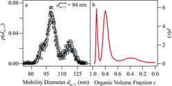
An example of the application of Equation (15)[15] for .p(ϵ; d)|_Gauss is shown in Figure 5 for a data set collected by a hygroscopic tandem differential mobility analyzer (HTDMA) (Smith et al. 2011, 2012, 2013). A particle population described by some f(d,t) was grown in the Harvard Environmental Chamber by the dark ozonolysis of α-pinene in the presence of ammonium sulfate seed particles. The seed distribution n₀(d) was measured by an SMPS. The mean reactor residence time τ was 14,100 s. The grown distribution n(d) was measured by an SMPS. The parameters β and λ (7.6 nm² s⁻¹ and 170 nm, respectively) were obtained by optimization of between the measured n(d) and that calculated by Equation (B1) of Kuwata and Martin (2012). For the HTDMA experiment shown in Figure 5, a particle subpopulation at a dry mobility diameter (+1 charge) of 84 nm was selected by a first DMA. For this subpopulation, .p(ϵ; d)|_Gauss was calculated by Equation (15)[15] . In the HTDMA experiment, the subpopulation was grown hygrocopically to 84% RH. Figure 5a shows the resulting number–diameter distribution that was measured (points). The dry mode of 84 nm resolves into three modes at higher RH. Figure 5b plots .p(ϵ; d)|_Gauss, showing three modes of organic volume fraction. These three modes explain the presence of three modes in the measurement at 84% RH (panel a) because the hygroscopic growth factor decreases for increasing organic volume fraction (note the reversal of the abscissa in panel b). The lines in panel a show the modeled number–diameter distribution at 84% RH based on calculated .p(ϵ; d)|_Gauss and the hygroscopic growth factors of mixed particles of sulfate and α-pinene SOM (Smith et al. 2011). There is excellent agreement between the measured (points) and modeled (lines) number–diameter distributions at 84% RH, supporting the validity to the calculated .p(ϵ; d)|_Gauss.

FIG. 5. Data set of a number–diameter distribution measured by a hygroscopic tandem differential mobility analyzer for data collected during the study of Smith et al. (2011). See main text for further discussion.

In addition to the equations developed herein for a focus on condensational growth in a CMFR, the Appendix presents a generalized form of p(ϵ;d) applicable to any steady-state flow through reactor (e.g., laminar-flow reactors, plug-flow reactors of variable dispersion, or any reactor of arbitrary but known distribution for particle residence times) in which particles undergo condensational growth according to any governing equation on a number–diameter distribution n₀(d) of seed particles.

Applications of the generalized equations can also be used to approximate atmospheric processes under particular applicable scenarios, such as large urban regions that emit primary particles that are subsequently mixed and coated during downwind transport by secondary gas-to-particle processes. For this case, the probability density function of particle residence time follows from the coupling of atmospheric eddies with Lagrangian transport, corresponding to a plug-flow-reactor with dispersion (Dragoescu and Friedlander, 1989). In the case that growth rates are known, effective residence times (i.e., time zero at urban emission of the primary particle) are obtained by inverting size-resolved chemical measurements. Alternatively, effective residence times are obtained by the known decay rates of measured gas-phase species.

FUNDING

This study was supported by the Office of Science (BES), U.S. Department of Energy, Grant No. DE-SC0006677, and by the U.S. National Science Foundation, Grant No. AGS-1249565. Mikinori Kuwata was supported by the Japan Society for the Promotion of Science (JSPS) postdoctoral fellowship for research abroad.

SUPPLEMENTAL MATERIAL

Supplemental data for this article can be accessed on the .

APPENDIX

A generalized form of p(ϵ;d) can be developed for any steady-state flow through reactor having a known or measured distribution p_t(t) of particle residence times. The equation is as follows (see the SI): [A1]

This equation is a generalized version for any growth law and any residence time distributions for different types of steady-flow flow-through reactors. Particle growth occurs on a number–diameter distribution n₀(d) of seed particles by gas-phase condensation, heterogeneous interfacial chemistry, or any other mechanism so long as I(d) > 0 for all d. A condition for use of this equation is that the residence time distribution p_t(t) must not depend on d₀. Further governing conditions and assumptions are discussed in more detail in Kuwata and Martin (2012).

As a check in Equation (A1), use of Equation (6)[6] for t, i.e., for condensational growth (cf. Equation (1)[1] of Kuwata and Martin (2012) and of for a CMFR (Equation (4)[4] Kuwata and Martin [2012]) transforms Equation (A1) into the following: [10]

This result reproduces Equation (10)[10] .