Multivariate Characterization of a Continuous Soot Monitoring System Based on Raman Spectroscopy

Abstract

The demand for precise and continuous monitoring of air quality has increased. An important descriptor of air quality is the concentration of problematic carbonaceous particles responsible for diseases and climate change. The specific measurement of carbonaceous components in the air is still a topic in research and development. Here, we introduce an integrated and continuous soot monitoring system based on Raman spectroscopy. In comparison to the often utilized light absorption, Raman spectroscopy is capable of determining the graphitic microstructure found in carbonaceous particles. We present first measurements taken in a controlled environment contaminated with varying concentrations of diesel soot. The Raman bands of soot turn out to be tightly mixed up with signals from secondary physical factors. In order to evaluate the data, multivariate methods are applied. After determination of the latent variables using principal component analysis (PCA), the system is further rotated using a linear discriminant analysis (LDA)-criterion and a subsequent nonlinear iterative partial least squares (NIPALS)-like step. One of the variables obtained by this methodology can be shown to exclusively describe the optical filter loading while the orthogonal factor space allows for conclusions on the secondary factors.

Copyright 2015 American Association for Aerosol Research

INTRODUCTION

Carbonaceous micro- and nanoparticles in the atmosphere, especially those coming from incomplete combustion, are responsible for respiratory and cancerous diseases (Smith et al. 2010; Shiraiwa et al. 2012). Monitoring the concentration of these particles may help choosing countermeasures or understand their distribution and sources better. There are already densely meshed measurement points of local agencies monitoring the total particulate matter (PM). The PM, however, among soot also includes further components like nitrates or biomatter, which can account for a great part of the values measured (Kuhlbusch et al. 2004; Bressi et al. 2013). Recent aethalometers allow for source apportionment regarding organic and elementary carbon (Sandradewi et al. 2008; Drinovec et al. 2014). Still, a more specific monitoring would be most helpful.

While the term “black carbon” describes particles in terms of electromagnetic absorption properties relevant for atmospheric research, “soot” rather denotes carbonaceous fractions of PM produced by incomplete combustion (Petzold et al. 2013). Atmospheric soot is typically found as agglomeration of primary particles of sizes ranging from 5 nm to about 100 nm (Psfai et al. 1999; Su et al. 2004). These primary particles consist of turbostratically stacked graphene-like layers (Clague et al. 1999), which cause the unique Raman spectrum. An ideal graphitic lattice would show only the so-called “G” - Raman line at 1575 cm⁻¹ (Tuinstra and Koenig 1970) (G for graphit). Distortions and discontinuities of the graphitic lattice are assumed to cause additional vibrational modes summarized by the so-called D-bands around 1350 cm⁻¹ (D for distortion). These band parameters are discussed to be connected to different material properties like degree of graphitization, amount of amorphous and organic carbon, and oxidation history (Escribano et al. 2001; Sze et al. 2001; Knauer et al. 2009). Based on the band parameters, different particle types and sources can be discriminated (Rosen and Novakov 1978; Dippel and Heintzenberg 1999; Sadezky et al. 2005; Agudelo et al. 2014).

In environmental monitoring, Raman spectroscopy has been applied by Mertes et al. to detect “graphitic carbon” in atmospheric aerosols deposited on glass fiber filters (Mertes et al. 2004). Here, a value was obtained by integrating the Raman-intensities between 1510 cm⁻¹ and 1736 cm⁻¹ after normalization and subtraction of a filter-only spectrum. Ivleva et al. performed a very comprehensive study of atmospheric particles collected with an electrical impactor (Ivleva et al. 2007). Spectral analyses have been carried out using both spectral libraries and the fitting of a band model. As a result, different sources of carbonaceous particles could be discriminated and further fractions like nitrates and sulfates could be identified.

The applicability of Raman spectroscopy for the analysis of atmospheric aerosols and especially their carbonaceous components has been demonstrated. However, in most works, stationary and expensive high-end Raman microscopes are used to acquire the spectra while the aerosol sampling is accomplished offline with the specimen being analyzed in a laboratory afterward. This approach requires learned personnel and naturally lacks high throughput. The time spared using a continuous and fully automated measurement system could otherwise be invested into evaluation of data. Furthermore, the attempt of a full automatization probably leads to challenges usually not encountered in laboratory-environments. With this in mind we developed the Raman Soot Spectrometer (RaSoS) presented here. Since Raman spectroscopy provides no internal standard and the expected signal-to-noise ratio (SNR) is rather low during field operation, the methods of data evaluation are of great importance.

A common evaluation method for Raman-spectra of soot and related carbonaceous substances is the nonlinear fitting of multiple Raman bands. Best matches and lowest errors of fit have been achieved using the 5-Band model proposed by Sadezky et al. (2005), which includes the G-peak and four D-peaks. However, it was also stated that the nonlinear fitting procedure bears statistical uncertainties (Ivleva et al. 2007). Under non-laboratory circumstances, there are even additional system- and process-based errors contributing to unexpected spectral behavior. Therefore, the less constrained multivariate methods are used for our first data analysis.

Multivariate statistical methods are widely used for calibration and classification purposes in spectroscopy. While the regression and calibration methods such as classical least squares (CLS), inverse least squares (ILS), and partial least squares (PLS) are rather known in the domain of spectroscopy and chemometrics (Massart et al. 1988), principal component analysis (PCA) and linear discriminant analysis (LDA) are also popular in the fields of pattern recognition and machine learning, where not only the scores but also the model itself is derived from the dataset. A look onto both model and scores may reveal underlying coherencies initially not considered or confirm assumptions made beforehand (Haaland and Thomas 1987; Haaland et al. 1990). In this work, the data acquired by the RaSoS are first analyzed by means of exploratory factor analysis using PCA. Based on the structure found in the data, the decision is made to further evaluate the factors using supervised pattern recognition in form of the LDA.

METHODS

RaSoS

The current prototype of RaSoS is an integrated system comprising laser, optics, spectrometer, aerosol sampler, filter supply, pump, actors, a computer, the power supply, and further peripheral components. All components are encased in a 19” housing with 4 height units so that the RaSoS can be easily installed in measurement containers (Figure 1).

FIG. 1. Overview of the RaSoS integrated system. (a) The housing suited for 19” racks. (b) The analytical unit.

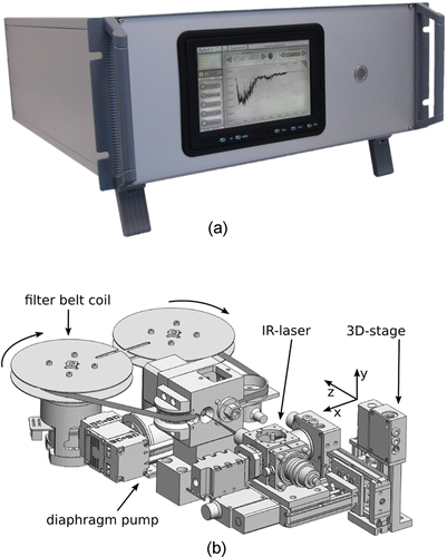
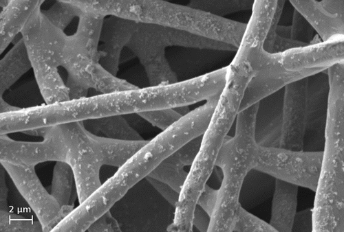
Due to their low concentration, atmospheric particles are difficult to be analyzed using Raman spectroscopy without previous local deposition. For that purpose, filtering separators are widely used (Sze et al. 2001; Mertes et al. 2004; Knauer et al. 2009). There are many demands on the filter material: It must satisfy spectroscopic as well as mechanical constraints while supporting the goal of automatization. We have tested 12 filters of different types (membrane, fiber, surface) and materials (glass, metal, paper, polymer) and have chosen a metal fiber filter (Bekaert GmbH, Belgium) showing low inelastic scattering while being mechanically resilient and chemically inert. The densely meshed metal filaments are of 2 µm diameter on the one side (Figure 2) and 4 µm on the other side. We use the 2 µm side for deposition. The filter is 250 µm thick.

FIG. 2. SEM-image of a moderately loaded filter.

The aerosol is sampled by a diaphragm pump with a flow-rate of 6 l/min through 4 mm antistatic tubes. At the first stage of the aerosol sampler (Figure 1b), the particles are separated onto the filter tape within a spot size of 6.5 mm. The coated spot then is transported to the second stage, where the spectroscopic acquisition is performed. At the same time, aerosol can be sampled on a new spot of a filter band for a semi-continuous monitoring. During the deposition and spectroscopy, the filter is pushed against the inner wall of the sampler by an elastically supported stamp. This ensures impermeability of the flow channel as well as a well-aligned filter surface for spectroscopy.

In front of the sampler, a three-dimensional (3D) motorized linear stage is positioned. On the stage, the laser and the confocal optics are mounted. This enables the illuminated spot to be moved across the filter surface as well as the adjustment of the focus. For excitation, a diode laser (QUIOPTIQ) with a wavelength of 785 nm and a maximum power of 80 mW is used. The long wavelength helps suppressing fluorescence, which has been reported to be a great obstacle in robust spectral acquisition (Ivleva et al. 2007). The linewidth is further reduced by a line filter (SEMROCK). Light is focused and collected by a 12 mm lens with f = 25 mm. A dichroic mirror (SEMROCK) separates the elastically scattered light from the Stokes-shifted parts, which are then coupled into a 100 µm multi-mode optical fiber. A spectrograph (Andor Shamrock 163) with a blazed grating containing 1200 l/mm and a thermoelectrically cooled (TEC) charge coupled device (CCD)—Camera (Andor iVac 316) disperse and record the spectrum. The grating of the spectrograph is adjusted to image wavelength-shifts ranging from 480 cm⁻¹ to 1790 cm⁻¹. That way, also the Raman band of the piece of monocrystalline Si at 520 cm⁻¹ installed at the front of the analytical unit can be recorded for reference.

An x86 mini—Integrated Technology Extended (ITX) computer running Linux controls all devices and is the host for the RaSoS-software written in C++. Different software modules provide sequencing and control for various types of measurements.

MULTIVARIATE ANALYSIS

The narrow spikes in the spectrum caused by incident cosmic rays can cause high variance and thus have to be removed beforehand. The data are preprocessed by a minimally manipulating median-based removal of the these spikes aswhere I(x) is the intensity of a spectrum at CCD line x, I_N(x) is the intensity of the same spectrum normalized to unit vector length, t is a threshold, ΔI = ||I_N,M(x) − I_N(x)||, and the median value I_M within a window w of the original or normalized spectrum

The normalization ensures the same behavior for different overall intensities for the same set of parameters [w,t] and the same spectrum length.

Prior to dimension reduction, the dataset is centered by subtracting the mean spectrum from the dataset. The mean spectrum represents common information, which otherwise would taint the results. It is common to subtract a baseline from the spectra. We deliberately forego this step for explorative analysis, since a reliable model for the baseline is not known and moreover would be difficult to fit. As a result, we plan to get a clear view onto the data.

A PCA can be described as a consecutive orthogonal rotation of the original manifest dataspace into the directions of highest variance. Due to the variance criterion, the first principal component (PC) rather hold substantial information, while the lesser components describe increasingly less contiguous information like noise or other random influences. By taking into account only the first few components, the number of variables can be reduced dramatically. Solely due to their low number, these new latent variables along with their loadings on the original manifest space help analyzing the data. In this work, the singular value decomposition (SVD) is used as algorithm. The term “score” is used for the actual value of a latent variable like the PCs.

When treating multivariate data in spectroscopy, partial least-square regression (PLSR) is a commonly used tool (Massart et al. 1988). Like the PCA, PLS finds an orthogonal set of latent variables. However, instead of the coordinate system being rotated according to a data-intrinsic variance criterion, the covariance of the data with a known factor is regarded. Given that, the PLS can also be considered as a method for supervised pattern recognition (Haaland and Thomas 1987). Due to the intentionally high covariance of the PLS-components regarding the outer variable, a regression onto that variable is prone to overfitting. In order to find a reasonable number of components, a leave-one-out (LOO) validation is applied. We use the kernel algorithm (Dayal and MacGregor 1997; Mevik and Wehrens 2007) for the PLS.

In PLSR, the obtained variables are used for least squares (LS)—regression against the outer variable. A regression with any variables can as well be seen as a supervised pattern recognition method that finds a direction with best (in terms of least squares) linear mapping properties with respect to the regressor.

The direct interpretation of PC or PLS scores and loadings can be difficult, since the variance-based rotation does not necessarily denote real factors of interest. On the contrary: multiple factors causing similar magnitudes of variance in the manifest space are rather summarized by single PCs. Thus, when interpreting single PCs without regarding the context of the other components simultaneously, misinterpretations may be the consequence. There are various methods for rotating systems into more meaningful orientations. Using manual rotation while projecting the scores onto two dimension (2D) allows the operator himself to reveal arbitrary structures and decide for further evaluation strategies (Cook et al. 1995). Computational rotation criteria only regarding the loadings have gained some attention in spectroscopic analysis (e.g., Varimax, which maximizes the variance along the loading vector, Kaiser 1958). However, tests with our data did not lead to any helpful directions. In contrast to Varimax et al., there are methods that host rotation criteria fed by the scores (projection pursuit, Cook et al. 1995; independent component analysis, ICA). Multivariate curve resolution (MCR) regards both scores and loadings by introducing constraints like non-negativity while being fed with the original data (Tauler et al. 1995). Not all of these methods are restricted to orthogonal rotation.

The LDA finds a linear combination a of a given set of variables, which best separates a priori known classes. This is done by maximizing the between-class variances B while keeping the within-class variances W low (Fisher 1936). The Fisher discriminant can therefore be obtained by maximizing a^TBa/a^TWa. When the input variables are rescaled such that the within-class covariance matrix W holds unit variances, the problem reduces to a^TBa, which corresponds to finding the eigenvalues of B (Venables and Ripley 2002). The resulting eigenvectors are the linear discriminants.

The LDA is commonly used for classification, for example, the assignment of an unknown test object to a set of previously defined and modeled classes. In our analysis, the Fisher criterion is used within the PC-space to yield directions of interest. Seen in the upper context, it can be regarded as rotation criterion fed by the PC-scores, whereas features are extracted, which best distinguish observations known to be different from each other.

As the linear discriminant (LD) is a linear combination of the original axes, orthogonality to these axes is not assured. To realign the full factor space orthogonally, a manual NIPALS-like (nonlinear iterative partial least squares) step (Wold 1966) is applied: First, the information hold by the LD is removed from the data (either in manifest or in latent space). The residuals are then decomposed again using an SVD. Virtually, the LD-axis is fixed while the remaining axes are again rotated into the directions of maximum variance. This ensures a component system being linearly independent, which is a good starting point for further interpretation of the factors.

For visualization and qualitative comparison, some variables are shifted to zero mean and scaled to unit vector length beforehand.

SAMPLING AND SPECTRAL ACQUISITION

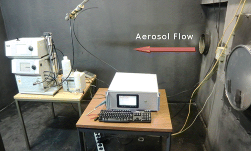
The measurements presented in this article have been run at the testing facility of “Institut für Gefahrstofforschung” (Institute for the Research of Hazardous Materials), which is located in the West of Dortmund, Germany. The exhaust of an idle diesel motor is led through a tube approx. 10 m long for laminarization of the air flow. The tube ends in a 10 cm³ measurement chamber, which is put under subpressure to suck in the aerosol (Figure 3). A flapper valve at the front of the tube is used to steplessly mix the diesel exhaust with fresh air from the outside. The RaSoS is placed on a table in the mid of the measurement chamber. Next to our system, a scanning mobility particle sizer (SMPS, TSI, Shoreview, MN, USA, Model 3080) comprising a condensation particle counter (CPC, TSI, Model 3010) is installed for reference. The differential mobility analyzer (DMA) column is set up to let submicron PM pass to the CPC. A sheath air mix ratio of 10:1 predilutes the high particle concentrations. The inlet tubes of both devices are hung up in the center of the chamber. Both devices have been set up for remote control and readout. Before sampling, the diesel motor has been warmed up for at least half an hour and the CPC readings have been given time to settle within 300 cm³ for each position of the flapper valve.

FIG. 3. Setup consisting of the RaSoS and a CPC in a measurement chamber flowed by the aerosol.

In order to gather a representative Raman signal from the whole filter area, the motorized stage is programed to move the laser spot of approx. 20 µm to 100 µm across the filter in a meander-like pattern during spectral acquisition. The quadratic pattern with 18 points and an edge length of 3.7 mm covers 37 mm of travel path. The lateral stage speed is kept constant at a relatively high speed of 1300 µm/s to reduce a heating up of the specimen. At the beginning of each spectral acquisition, the stage starts scanning from the first point of the pattern.

Both outer factors, the particle concentration measured by the CPC and the deposition time, are assumed to have a linear impact on the final filter loading. However, with raising filter loading, the probability of new particles covering each other rises exponentially, resulting in nonlinear behavior. Thus, multiple occupancy of the filter material should be minimized for quantitative analysis. In order to find an ideal deposition time t_d, an incremental deposition series was run first; starting with the measurement of an empty filter spot, the filter is moved back, coated, and then moved forward to the laser area again to take another spectrum. Given a fixed deposition time, this procedure is repeated 10 times while the particle concentration is kept constant at 237,000 cm³. A laser power of about 14 mW and an exposure time of 60 s were chosen for the incremental series. The focus was adjusted to meet the surface of a sparsely coated filter. The actual z-position previously was obtained by a depth series on the filter with the stage running the meander pattern.

In a second step, the deposition time was fixed to the value obtained by the incremental series so that multiple occupancy is low. Only the particle concentration was varied between 10,000 cm³ and 234,000 cm³, with 10,000 cm³ being the outside particle concentration. The exposure time has been raised to 120 s. The other parameters were the same as during the incremental series. Between 48,000 cm³ and 110,000 cm³, the flapper valve has been steadily opened. The other measurements have been taken with constant CPC values.

RESULTS AND DISCUSSION

Raw Spectra

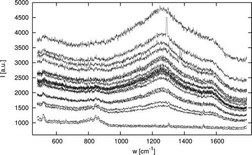
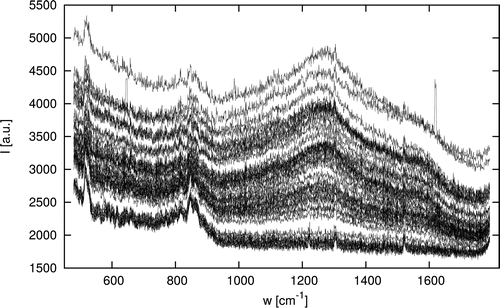
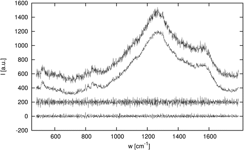
Figure 4 shows the raw spectra of two incremental series each comprising 10 sequential deposition steps of 2 min. The two bottom spectra show the pure filter signal, which consists of some narrow features between 510 cm⁻¹ and 844 cm⁻¹ and two small peaks at 1302 cm⁻¹ and 1520 cm⁻¹. With increasing filter loading, the characteristic soot G- and D-band intensities rise. The spectral underground and a slope toward the laser line seem to increase as well, both indicating fluorescence or high elastic scattering. As for the latter, parts of the reflected excitation line could still pass the optical filters and superimpose the faint Raman signal (Nalpantidis 2009).

FIG. 4. Raw spectra of the incremental series.

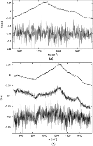
The high frequency noise usually would be accounted for a low signal intensity or readout errors of the CCD, decreasing with rising exposure times or SNR. In our measurements, however, a higher total signal strength is accompanied by a growing amount of these noisy features: The standard deviation of a noise profile, which was obtained by applying a Fast Fourier Transform (FFT)—highpass from 1/17.68 cm upward, strongly correlates with the mean values of the spectra (σ_xy = 0.985). Furthermore, the mean spectrum over all measurements reveals a non-statistical nature of the high-frequency component (Figure 5). Neither Raman-scattering, nor fluorescence is likely to produce such narrowly shaped wavelength shifts. Also, when analyzing a bulk of monocrystalline silicon or a cuvette of acetone with our system, such features are not being observed. This behavior could be explained by the substance-specific higher ratios of Raman- to elastic scattering cross-section and the high exposure times needed for a soot occupied filter, respectively. Hence, as a response to strong incident elastic scattering, either transmittance properties of the optical filters used in the RaSoS could be exposed or parasitic scattering hits the CCD array directly.

FIG. 5. Comparison of the noise profiles of a spectrum with t_d = 6 min, the mean spectrum (both subtracted with a linear baseline), and the corresponding noise profiles (from the top, with offsets). The standard deviations of the noise are σ_6min = 27.5 and σ_mean = 13.5 a.u.

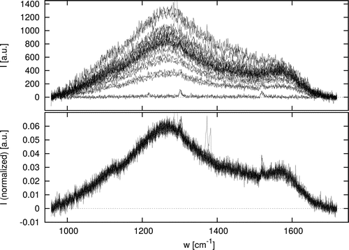
Figure 6 shows the spectra within an area cropped to [925 cm⁻¹, 1750 cm⁻¹] and subtracted with a linear baseline. It is mainly the Raman signal that should affect the data now. Normalizing the spectra to unit vector length unfolds similar qualitative features for all deposition times. This is conclusive as there should be only one type of soot particles coming from the idle diesel motor. The upper graph of Figure 8 shows the vector lengths over deposition time. Within the first 4 min, the intensities rise linearly with deposition time and there is little deviation between the two incremental series. At higher deposition times, however, the deviation is huge and the Raman intensities do not seem to reliably describe the filter loading anymore.

FIG. 6. Top: cropped and baseline-corrected spectra of the incremental series. Bottom: the same spectra except t_d = 0, normalized to unit vector length (intensity).

FIG. 9. By PCs explained variance of the incremental series.

Multivariate Analysis

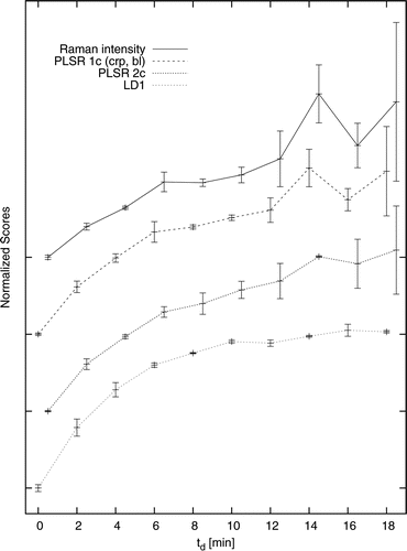
As a first approach, a PLSR is applied to the data. LOO-validation results in lowest errors for one component with the cropped and baseline-corrected data (Figure 6) and for two components with the untreated data. A PLSR is then applied to the full dataset using the previously determined number of components. When considering the final regression vectors (Figure 7), the chosen number of components seems to be appropriate, as with higher number of components mainly noise features are used for regression. The PLSR scores are shown in Figure 8. Using the pretreated spectra, the scores are very similar to the Raman-intensities. In case of the untreated data, the mean scores are more stable even at higher deposition times.

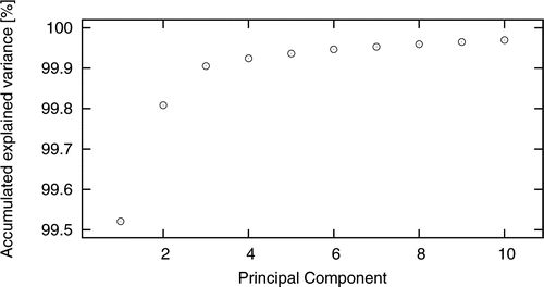
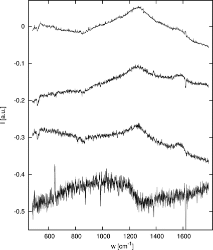
After applying a PCA to the untreated data, the first three PCs explain 99.91% of total variance (Figure 9). Most of the variance is caused by the spectral offsets, which are described by PC1. The G- and D-bands of soot are found in all PCs, whereas PC1 shows prominent intensities at the D-band position (Figure 10). Slope, filter features, and the noise discussed earlier show up in all loadings. Subsequent to PC3, only high frequency noise or spikes can be found, which confirms a number of three significant factors. However, as soot-specific signals appear in all three components, a direct interpretation of a single component is still not possible.

FIG. 10. Loadings of PC 1 to 4 of the incremental series with −0.1 offsets, from the top. PC1 was shifted to zero mean and scaled to unit vector length.

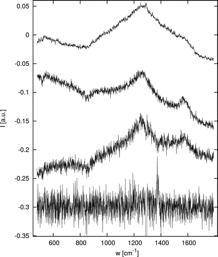
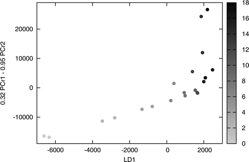
FIG. 11. PC1 and PC2 scores of the incremental series, shaded according to the deposition time in minutes.

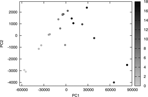
When viewing the measurements within their first two PCs (Figure 11) or better, in an interactive 2D-projection of all three PCs, a direction is apparent, which best describes the factor of deposition time. In order to determine that direction, a multiclass linear discriminant criterion is applied to the PC-system. The class memberships are derived from the deposition time, which implies a total count of 10 classes. The LDA yields a discriminant direction (LD1), which explains 99.13% of the inter-class variance. It loads on the original PC-system as 0.0615, 0.8008, and 0.5958. To orthogonally realign the former PC-axes with the newly defined LD1, a manual NIPALS-like step is run by subtracting LD1 from the dataset, followed by an SVD of the residuals. The resulting system (LD1, PCr1, PCr2) holds the same information as the original PC-system but allows for a better interpretability, as the LD1-axis is aligned with a known factor.

FIG. 12. Rotated components LD1 (0.6%), PCr1 (99.15%), and PCr2 (0.17% of variance) with −0.1 offsets, from the top. PCr1 was shifted to zero mean and scaled to unit vector length.

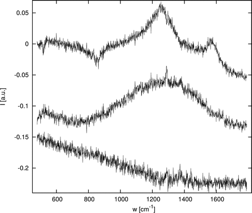
As a result, only LD1 appears to describe the Raman bands of soot (Figure 12). Additionally, inverted filter-specific features can be found in LD1 only. The latter can be attributed to opaque particles covering the filter material. Both physical effects are exclusively found in LD1 while acting complementary to each other. This leads to the assumption that the factor coincident with LD1 is the “single-occupancy” or “optical filter loading.” The scores of LD1 first increase almost linearly with deposition time. With rising occupancy, the intensity is flattening out until representing that of a bulk mass of particles (Figure 8).

FIG. 13. Scores of the incremental series factor system after LDA-based rotation. (a) PCr1 first rises linearly with LD1 until the filter loading gets too high. (b) The deviation of PCr2 increases with higher optical filter loading.

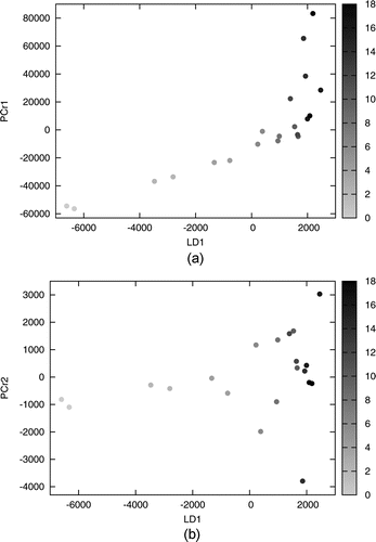
The residual components PCr1 and PCr2 span the space for observed effects secondary to the discussed optical filter loading. Similar to the former PC1, PCr1 still contains most of the dataset variance (99.15%) due to its strong offset. Its scores rise linearly with LD1 but show great outliers on high filter loadings (Figure 13a). With higher filter loadings, the number of soot particles within the laser spot increases. At the same time, the thermal isolation of single particles rises due to the filter cake and an increased distance to the metal filter matrix. Both factors lead to higher probabilities for the particles to heat up, eventually causing them to flash up in combustion. The resulting emission-based response could account for the high spectral variance.

FIG. 8. Normalized mean values and standard deviations of the incremental series scores from different evaluation methods: Raman intensities, PLS scores of untreated spectra using two components, PLS scores of cropped and baseline-corrected spectra (Figure 6) using one component, and the scores of LD1.

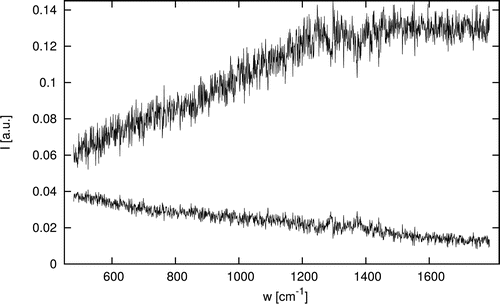
When further exploring the rotational ambiguity of PCr1 and PCr2, less complex directions can be found. Figure 14 shows the system rotated by 71.5° (PCr1 into direction of PCr2). The second component mainly comprises an offset and a slope toward the laser line, which indicates fluorescence or high elastic scattering. The first component represents a slope toward higher wavelengths, which may be caused by thermal radiation (Figure 15). The strong coincidence of both factors as well as the initial linear growth with the filter loading confirms an occasional ignition of particles rather than a continuous heating-up. On high filter loadings, the probability of bigger agglomerates to ignite significantly increases, leading to extremely high spectral responses.

FIG. 16. Spike-filtered spectra of the deposition series taken in 2  × 10 sequential deposition steps, each with a deposition time of 2 min.

FIG. 17. PCA-loadings of the deposition series with −0.1 offsets. PC1 was shifted to zero mean and scaled to vector length 1.

Deposition Series

The deposition series consists of 45 spectra (Figure 16) and the associated particle concentrations measured with the CPC. According to the results from the incremental series, a deposition time of 2 min was chosen to minimize multiple occupancy. The exposure time of 120 s results in an approx. doubled signal intensity compared to the incremental series taken with t_e = 60 s.

FIG. 18. Loadings of the rotated components LD1 (1.46%), PCr1 (97.51%), PCr2 (0.64%), and PCr3 (0.05% of variance) with −0.1 offsets, from the top. PCr1 was shifted to zero mean and scaled to unit vector length.

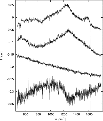
The first four principal components explain 99.66% of total variance. Their loadings look similar to those from the incremental series, although a fourth component showing noteworthy features exists (Figure 17). In order to trace the factor of optical filter loading within PC1-4, an LDA is applied again. Spectra with identical CPC values were assigned to an own class, which results in 14 different classes. The first linear discriminant (LD1) covers 99.67% of inter-class variance and loads on the PCs with 0.0936, 0.6767, 0.7161, and 0.1435. A variance-based rotation of the residuals yields the remaining three axes (PCr1-3).

FIG. 19. Zero mean shifted and unit vector scaled Raman intensities from spectral area and LD1 scores of the deposition series. The two plots are vertically shifted for better visibility. The dotted lines show the respective linear LS-fits.

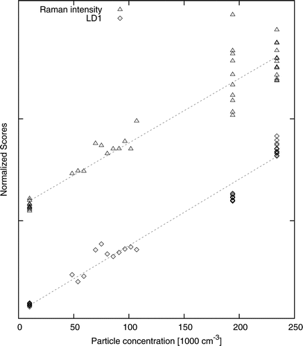
The Raman signal of soot as well as the inverted filter features can again be isolated in LD1 (Figure 18). Compared to the Raman intensity gained by the vector length of the cropped and baseline-subtracted spectra (as applied above), the LD1 scores show less deviation especially at higher filter occupancies while maintaining the correlation to the measured CPC values (Figure 19). This corresponds well to the observations previously made on the incremental series, after which additional factors like sample heat up and particle ignition interfere with the Raman signal. The remaining variance of LD1 could result from the meander path, which covers only a small subset of the whole spot area and may include or leave out single agglomerates. This issue could be addressed by a rotation of the pattern after each run. Another reason for the LD1 variance could be a modification of the deposited particles (e.g., graphitization or combustion).

FIG. 14. Loadings of the 71.5° rotated PCr1 and PCr2. Variances explained are 10.1% and 89.2% (from top down).

FIG. 15. The scores of the supposed heat-component gained by rotation of PCr1 and PCr2, plotted against LD1.

SUMMARY AND CONCLUSIONS

The Raman soot spectrometer was introduced and first measurements of a soot contaminated aerosol were presented. The spectra show the typical Raman bands of carbonaceous materials. Quantitative evaluation was attempted using conventional methods like a spectral integral after baseline-subtraction as well as a PLSR. The results showed poor correlation with the expected filter occupancy and motivated further analysis using tools from the domain of classification and pattern recognition.

The resulting scores and models could help to both isolate the factor of filter loading along with the Raman signals and understand effects secondary to the Raman scattering better. A disruptive factor probably caused by ignition of particles overlaps the Raman bands of soot (Figure 12 and 18), leading to inaccurate Raman intensities when calculated by conventional means (i.e., baseline and spectral area). The attenuation of filter features caused by opaque particles aided unscrambling the factors. It was shown that the attenuation acts approximately complementary to the Raman scattering, which itself is a proof for the Raman intensity being proportional to the filter loading. Evaluation of the deposition series showed good correlation of the extracted factor with the particle concentrations simultaneously measured with the CPC and demonstrated the suitability of the introduced system for quantitative analysis of the aerosol.

By freely utilizing and combining tools from classical calibration, explorative factor analysis and pattern recognition, complex and noisy signals could be decomposed into descriptive factors. As the outer variable fed to the LDA is not regarded as ordinal, nonlinearities in the data or measuring errors do not tarnish the results as they do, for example, in the case of the PLSR, which allows for a generic recognition of structure. Furthermore, the model-free approach separates interfering signals, which during band-fit procedures would have been interpreted as Raman bands of soot.

The multivariate tools presented may serve as basis for a robust calibration of the RaSoS in the future. We hope to successfully apply the multivariate tools evaluated here equally to the spectra of complex multicomponent aerosols. This way, factor directions coincident with concentrations of different kinds of soot, PM, or further aerosol components could be found and regarded for subsequent calibration steps. In addition to the use of multivariate methods, system parameters like laser power, focal plane, and exposure time should be further optimized to both reduce the impact of secondary factors like sample heat up and improve the SNR.

NOMENCLATURE

CCD	=	charge coupled device
CLS	=	classical least squares
CPC	=	Condensation particle counter
DMA	=	Differential mobility analyzer
FFT	=	Fast Fourier transform
ICA	=	Independent component analysis
ILS	=	Inverse least squares
ITX	=	Integrated technology extended
LD	=	Linear discriminant
LDA	=	Linear discriminant analysis
LOO	=	Leave-one-out
LS	=	Least squares
MCR	=	Multivariate curve resolution
NIPALS	=	Non-linear iterative partial least squares
PC	=	Principal component
PCA	=	Principal component analysis
PCr1	=	Principal component 1 (from residuals)
PCr2	=	Principal component 2 (from residuals)
PLS	=	Partial least squares
PLSR	=	Partial least-square regression
PM	=	Particulate matter
RaSoS	=	Raman soot spectrometer
SMPS	=	Scanning mobility particle sizer
SNR	=	Signal-to-noise-ratio
SVD	=	Singular value decomposition
TEC	=	Thermoelectrically cooled

Symbol Directory

te	=	Exposure time
td	=	Deposition time
σxy	=	Correlation coefficient
Td	=	Deposition time

FUNDING

The authors are grateful for funding by the Ziel2.NRW and EFRE programs.

Notes

¹ In our case, the space is spanned by the variables received from the 1650 CCD lines of the camera.

² When using Varimax, Quartimax, Oblimax, Quartimin: the resulting loadings still shared soot Raman-bands:

³ It is noteworthy, that when regressing on the principal components instead, the regression vector shows the same noisy features not until including the 7th component.

FIG. 7. PLS regression vectors (zero mean, normalized) when using a different number of components (top = 1 component, with offsets). (a) For cropped and baseline-subtracted data. (b) For the untreated data.

⁴ In a first step, the class memberships needed for the LDA could be derived from the always known deposition time.

REFERENCES

- Agudelo, J. R., lvarez, A., and Armas, O. (2014). Impact of Crude Vegetable Oils on the Oxidation Reactivity and Nanostructure of Diesel Particulate Matter. Combust. Flame, 161(11):2904–2915.
- Bressi, M., Sciare, J., Ghersi, V., Bonnaire, N., Nicolas, J. B., Petit, J. E., Moukhtar, S., Rosso, A., Mihalopoulos, N., and Fron, A. (2013). A One-Year Comprehensive Chemical Characterisation of Fine Aerosol (pm 2.5) at Urban, Suburban and Rural Background Sites in the Region of Paris (France). Atmos. Chem. Phys., 13(15):7825–7844.
- Clague, A., Donnet, J., Wang, T., and Peng, J. (1999). A Comparison of Diesel Engine Soot with Carbon Black. Carbon, 37(10):1553–1565.
- Cook, D., Buja, A., Cabrera, J., and Hurley, C. (1995). Grand Tour and Projection Pursuit. J. Comput. Graph. Stat., 4(3):155–172.
- Dayal, B., and MacGregor, J. (1997). Improved PLS Algorithms. J. Chemomet., 11(1):73–85.
- Dippel, B., and Heintzenberg, J. (1999). Soot Characterization in Atmospheric Particles from Different Sources by NIR-FT Raman Spectroscopy. J. Aerosol Sci., 30:907–908.
- Drinovec, L., Monik, G., Zotter, P., Prvt, A. S. H., Ruckstuhl, C., Coz, E., Rupakheti, M., Sciare, J., Mller, T., Wiedensohler, A., and Hansen, A. D. A. (2014). The “Dual-Spot” Aethalometer: An Improved Measurement of Aerosol Black Carbon with Real-Time Loading Compensation. Atmos. Meas. Tech. Discuss., 7(9):10179–10220.
- Escribano, R., Sloan, J., Siddique, N., Sze, N., and Dudev, T. (2001). Raman Spectroscopy of Carbon-Containing Particles. Vib. Spectros., 26:179–186.
- Fisher, R. A. (1936). The Use of Multiple Measurements in Taxonomic Problems. Ann. Eugenics, 7(2):179–188.
- Haaland, D., and Thomas, E. (1987). Partial Least-Squares Methods for Spectral Analyses. Anal. Chem., 60:1193–1202.
- Haaland, D., Higgins, K., and Tallant, D. (1990). Multivariate Calibration of Carbon Raman Spectra for Quantitative Determination of Peak Temperature History. Vib. Spectrosc., 1:35–40.
- Ivleva, N. P., McKeon, U., Niessner, R., and Poeschl, U. (2007). Raman Microspectroscopic Analysis of Size-Resolved Atmospheric Aerosol Particle Samples Collected with an ELPI: Soot, Humic-Like Substances, and Inorganic Compounds. Aerosol Sci. Technol., 41:655–671.
- Kaiser, H. (1958). The Varimax Criterion for Analytic Rotation in Factor Analysis. Psychometrika, 23:187–200.
- Knauer, M., Schuster, M., Su, D., Schlogl, R., Niessner, R., and Ivleva, N. (2009). Soot Structure and Reactivity Analysis by Raman Microspectroscopy, Temperature-Programmed Oxidation, and High-Resolution Transmission Electron Microscopy. J. Phys. Chem., 113:13871–13880.
- Kuhlbusch, T. A. J., Quass, U., Koch, M., Fissan, H., Bruckmann, P., and Pfeffer, U. (2004). PM10 Source Apportionment at Three Urban Back Ground Sites in the Western Ruhr-Area, Germany. J. Aerosol Sci., 35:79–90.
- Massart, D., Vandeginste, B. G. M., Deming, S. N., Michotte, Y., and Kaufman, L. (1988). Chemometrics: A Textbook. Elsevier Science B.V., Amsterdam, The Netherlands.
- Mertes, S., Dippel, B., and Schwarzenboeck, A. (2004). Quantification of Graphitic Carbon in Atmospheric Aerosol Particles by Raman Spectroscopy and First Application for the Determination of Mass Absorption Efficiencies. J. Aerosol Sci., 35(3):347–361.
- Mevik, B., and Wehrens, R. (2007). The PLS Package: Principal Component and Partial Least Squares Regression in r. J. Stat. Softw., 18(2):1–24.
- Nalpantidis, K. (2009). Qualitative und Quantitative Bestimmung von Rußaerosolen und Anderen Feinstuben auf Basis der Raman-Spektroskopie. PhD thesis, Ruhr-Universitt Bochum, Logos Verlag Berlin GmbH.
- Petzold, A., Ogren, J. A., Fiebig, M., Laj, P., Li, S. M., Baltensperger, U., Holzer-Popp, T., Kinne, S., Pappalardo, G., and Sugimoto, N. (2013). Recommendations for Reporting “Black Carbon” Measurements. Atmos. Chem. Phys., 13(16):8365–8379.
- Psfai, M., Anderson, J., Buseck, P., and Sievering, H. (1999). Soot and Sulfate Aerosol Particles in the Remote Marine Troposphere. J. Geophys. Res.: Atmos., 104(D17), 21,685–21,693.
- Rosen, H., and Novakov, T. (1978). Identification of Primary Particulate Carbon and Sulfate Species by Raman-Spectroscopy. Atmos. Environ., 12:923–927.
- Sadezky, A., Muckenhuber, H., Grothe, H., Niessner, R., and Poschl, U. (2005). Raman Microspectroscopy of Soot and Related Carbonaceous Materials: Spectral Analysis and Structural Information. Carbon, 43:1731–1742.
- Sandradewi, J., Prvt, A. S. H., Szidat, S., Perron, N., Alfarra, M. R., Lanz, V. A., Weingartner, E., and Baltensperger, U. (2008). Using Aerosol Light Absorption Measurements for the Quantitative Determination of Wood Burning and Traffic Emission Contributions to Particulate Matter. Environ. Sci. Technol., 42(9):3316–3323.
- Shiraiwa, M., Selzle, K., and Poeschl, U. (2012). Hazardous Components and Health Effects of Atmospheric Aerosol Particles: Reactive Oxygen Species, Soot, Polycyclic Aromatic Compounds and Allergenic Proteins. Free Radical Res., 46(8):927–939.
- Smith, K. R., Jerrett, M., Anderson, H. R., Burnett, R. T., Stone, V., Derwent, R., Atkinson, R. W., Cohen, A., Shonkoff, S. B., Krewski, D., III, Pope, C. A., Thun, M. J., and Thurston, G. (2010). Public Health Benefits of Strategies to Reduce Greenhouse-Gas Emissions: Health Implications of Short-Lived Greenhouse Pollutants. Lancet, 374(9707):2091–2103.
- Su, D. S., Mller, J. O., Jentoft, R. E., Rothe, D., Jacob, E., and Schlgl, R. (2004). Fullerene-Like Soot from Euro IV Diesel Engine: Consequences for Catalytic Automotive Pollution Control. Top. Catal., 30–31(1–4):241–245.
- Sze, S., Siddique, N., Sloan, J., and Escribano, R. (2001). Raman Spectroscopic Characterization of Carbonaceous Aerosols. Atmos. Environ., 35:561–568.
- Tauler, R., Izquierdo-Ridorsa, A., Gargallo, R., and Casassas, E. (1995). Application of a New Multivariate Curve Resolution Procedure to the Simultaneous Analysis of Several Spectroscopic Titrations of the Copper (ii)polyinosinic Acid System. Chemometr. Intell. Lab., 27(2):163–174.
- Tuinstra, F., and Koenig, J. L. (1970). Raman Spectrum of Graphite. J. Chem. Phys., 53(3):1126–1130.
- Venables, W. N., and Ripley, B. D. (2002). Modern Applied Statistics with S., 4th ed. Springer, New York.
- Wold, H. (1966). Estimation of Principal Components and Related Models by Iterative Least Squares. Multiv. Anal., 1:391–420.