A miniature scanning sun photometer for vertical profiles and mobile platforms

ABSTRACT

A miniature sun photometer has been developed that makes continuous almucantar scans to measure solar irradiance and sky radiance in four wavelength bands set by interference filters. It has a well-defined field of view and can rapidly compensate for a tilting platform. It weighs less than 400 g and has an average power consumption of less than 5 W. Together, these characteristics make it suitable for vertical profiles using small balloons or unmanned aircraft systems (UASs). Preliminary results are presented showing measurements of optical depth and the phase function of scattered sunlight. An optical depth of about 0.03 in a clean boundary layer was measurable with an accuracy of better than 0.01.

Copyright © 2016 American Association for Aerosol Research

EDITOR:

• Thomas W. Kirchstetter

Introduction

Sun photometers provide effective and geographically widespread measurements of optical depth (Holben et al. 1998; Kim et al. 2008). For aerosols, one goal of a sun photometer is to measure the direct solar irradiance with sufficient accuracy to determine the sunlight scattered out of the direct beam by aerosols. This yields the aerosol optical depth after accounting for the slant path through the atmosphere, Rayleigh scattering, and any gas-phase absorption. Useful measurements require an accuracy of 1% to a few percent. A secondary goal is often to measure the sky radiance. This contains important information about the aerosol particles. For example, the phase function can be used to constrain the size of aerosols because larger particles scatter more light at small angles than smaller particles.

An obvious but important limitation of ground-based radiometers such as AERONET is the lack of information on the vertical distribution of aerosols. Although vertical profiles of aerosols can be obtained from lidars, the inversion from backscatter to extinction is complicated. There is a fundamental simplicity to differencing the sunlight between different altitudes, especially if the optical depth is sufficiently low for a single scattering approximation. If 5% of the direct sunlight is lost in going from a higher to lower altitude, then the optical depth of that layer is 0.05 divided by the geometric (air mass) factor for the slant angle. At wavelengths with negligible atmospheric absorption, the only correction to derive aerosol optical depth is to account for Rayleigh scattering.

A group at National Aeronautics and Space Administration (NASA) Ames has developed a succession of airborne photometers that track the sun. Older versions had six or 13 filter channels (Matsumoto et al. 1987; Schmid et al. 2000). A newer version has complete spectral capability allowing the retrieval of O₃, NO₂, and other species, in addition to aerosol properties (Dunagan et al. 2013). Although more capable than the instrument described here, this instrument is much larger (much of an equipment rack) and is much more complex. It also takes more time to scan the sky. Karol et al. (2013) described a much smaller airborne sunphotometer with both visible and infrared filters that can track the sun from aircraft and other moving platform. Although smaller than other airborne photometers, the Karol et al. design is still many times the size of the instrument described here, a miniature Scanning Aerosol Sun Photometer (miniSASP). A miniature photometer based on light-emitting diodes (LEDs) (Mims 1992; Mims 2002) did not incorporate any sun tracking.

Instrument design

The instrument design was driven by a desire to keep the mass and power consumption suitable for either a radiosonde balloon payload or a Manta unmanned aircraft system (UAS) operated by the NOAA Pacific Marine Environmental Laboratory (Bates et al. 2013). Cost was also a consideration because balloon and UAS payloads are not always recovered. Therefore, some of the components are from hobby designs. The size and cost constraints not only force some undesirable trade-offs against performance but can also result in simple designs.

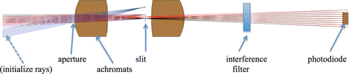
Rather than a filter wheel, there are four independent telescopes with an interference filter (Intor Inc.) for each channel (Figure 1). Each telescope has two 5-mm diameter lenses (Thorlabs AC050-008-A or B). These are achromats with less spherical aberration than singlet lenses. A 1.1-mm diameter front pupil limits the light entering the telescope. This pupil is imaged onto the detector for uniform illumination. A 390 × 1180-µm slit (custom, National Aperture) is placed at the focal point. This provides a 3° wide × 9° high field of view. The larger vertical dimension provides tolerance for the motion compensation of a possibly tilting mobile platform. A different field of view could be easily set with the appropriate slit or circular aperture. The most critical dimensions in the telescope are coaxial alignment, achieved by putting all components in a reamed hole, and the position of the slit relative to the first lens, which is set with a precision spacer. All four telescopes are in a single aluminum block. A small heater integrated with a temperature controller (ThermOptics DN505) minimizes condensation and keeps the photodiodes at an approximately constant temperature.

Figure 1. Optical design of one channel. Not shown are baffles after the first lens and before the interference filter. Shaded lines in the figure are to distinguish the angles rather than representing different colors of light. Chromatic aberration is too small to be seen on this scale.

The instrument is shown in Figure 2. One major simplification is that the instrument does not actively track the sun. Instead, it continuously scans the sky at the elevation angle of the sun, called an almucantar scan. The scan introduces several desirable features. First, only the elevation needs active tracking, not the azimuth. Second, the scans run in one direction, so backlash is minimized. Third, the instrument always obtains the phase function of sky radiance for a range of angles. Finally, the scans allow the subtraction of the sky brightness next to the sun from the sun measurement. This first-order correction allows the use of a larger field of view, which in turn eases tracking requirements and the dynamic range between the direct sun measurement and the sky radiance.

Figure 2. The radiometer assembly. For scale, the dome is about 5 cm in diameter. For flights, a thin plastic moving cover rides in the slot in the dome. The metal spur gear has been replaced by a nylon gear. The pupils for all four channels are visible on the front of the telescope.

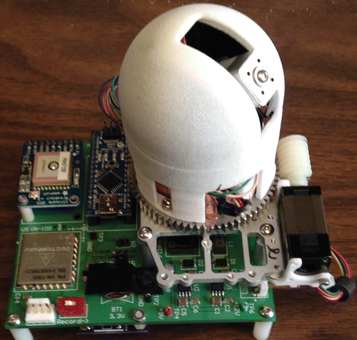
The azimuth scans are made with a stepper motor (Sanyo SH2141-5541) driving a 72- or 80-tooth horizontal spur gear. A worm gear gives a large speed reduction in a small space. A stepper motor is used to give a well-determined rotational speed. The elevation motor and the telescope yoke are mounted directly to the spur gear (Figure 2). A slip ring (Adafruit) allows continuous scans in one direction. A sufficiently small and simple encoder for the rotation could not be found. Therefore, a small photodetector (Sparkfun) aimed at a scribe mark on the bottom of the gear provides an index for each rotation and the azimuth is determined from the rotation of the stepper motor relative to either the scribe mark or the direct sun peak in the data. The elevation motor is a brushless servo positioner (Futaba BHS153 or equivalent) intended for radio-controlled airplanes.

The electronics mostly comprise commercially available modules. Commercial modules are used for the stepper motor driver (Pololu DRV8834), the GPS (Adafruit Ultimate GPS Breakout), a barometer (MS5607), and the attitude sensor (VectorNav VN-100). An exception is a small custom board containing the photodiodes (Hamamatsu S5972) and a quad 20-bit integrating current to digital converter (Texas Instruments DDC114). This board is mounted directly to the back of the telescope block. All of the motor control, timing, and data acquisition functions are handled by an Arduino Nano microcontroller board. The Arduino microcontroller includes counter-timer functions that can run without processor intervention. These timers are used to drive the stepper motor and create the pulse-width modulation for elevation servo. The Arduino reads the digitizer and other analog channels and puts out a logic-level RS232 data stream that is written to a memory card by a data logger module (Slerj SSR-LC-TH).

The elevation angle of the sun is computed by an Arduino subroutine that calculates the sun position from the GPS time, latitude, and longitude. For a moving platform, the Arduino also reads the pitch and roll of the instrument from the attitude sensor. It then computes how to correct the elevation motor to point at the same circle in the sky. This real-time tilt correction is updated at about 4 Hz, although the overall loop response is not that fast. To keep the code simple, a second-order approximation to the tilt correction is computed. This is highly accurate at low and moderate elevation angles. It does not handle special cases for large tilts when the sun is almost overhead, when, for example, a tilting platform can push the sun angle over the vertical into the opposite hemisphere.

A full azimuth revolution is made in about 30 s and measurements are made every 30 ms. This rate gives eight measurements as the 3° wide slit passes the sun so that a central value can be determined. The DDC114 current to digital converter architecture makes truly simultaneous measurements of all four channels with no readout dead time. For ground use, a somewhat slower rotation speed would be desirable (it would allow a smaller field of view), but during a vertical profile the rotation must be sufficiently fast so that the altitude change is minimal during one revolution. Each 30-ms measurement is divided into a 900-µs integration period and a 29.1-ms period. The longer integration period has less digitization noise and the shorter period is used when the current to digital converter saturates within 29 ms. The two periods are easily combined and data in the overlap region show near-perfect correlation between the short and long integrations.

The 30-s revolution time means that the best measurements are made if an aircraft or other platform is pointed in the same direction for at least 30 s. If the platform rotates, the slit will still scan across the sun but the data are more difficult to interpret because the turn adds or subtracts from the azimuth scan rate. Since there is continuous feedback for the elevation angle, the platform does not need to have a stable attitude for 30 s, just that the pitch and roll cannot overwhelm the tilt correction.

The 3° × 9° slit is larger than conventional ground-based instruments. The near-sun corrections are still small for most cases. For example, if the aerosol scattering is described by the Henley–Greenstein function with g ≈ 0.75, about 2% of the scattered light goes through the slit and would be counted as direct sunlight. In this case, a layer aerosol optical depth of 0.1 could be measured as 0.098. However, a correction for sky radiance during the direct sun signal can be made by interpolating the signal from each side of the sun and subtracting the result from the direct sun signal. If one looks 5° to each side of the sun, the interpolation of the g ≈ 0.75 Henley–Greenstein function matches the true correction to within about 10%. In the example here of a layer optical depth of 0.1, correcting with an interpolated signal would yield an error due to slit size that would be small compared with other errors. The correction may get more difficult in high optical depth situations when multiple scattering is important or when thin clouds are present. A larger slit size will make it more difficult to retrieve the size distribution of large particles from the phase function of light scattered at small angles.

Sample data

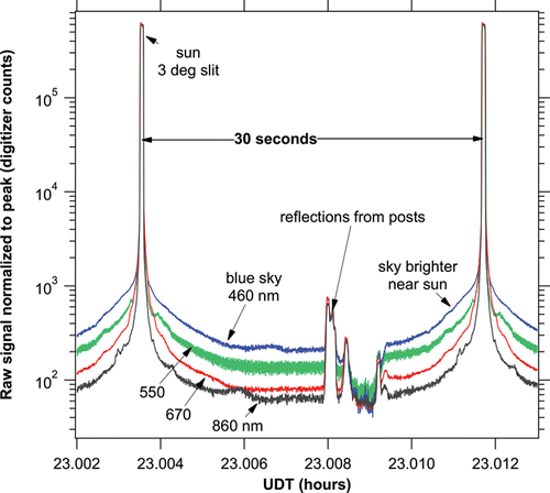
The output of the photometer is a time series of simultaneous measurements at four wavelength bands along with housekeeping information such as the barometric pressure and the GPS position. For these measurements, the interference filters had 10-nm bandwidths centered at 460, 550, 670, and 860 nm for measurements in the blue, green, red, and near-infrared. Out of band, blocking is specified as at least 10⁴. Figure 3 shows about 40 s of signal. The long and short integration periods have been combined into a single time series. Even with sampling every 30 ms, the sky measurements have good signal to noise. The small bump in the 860-nm channel just before 23.006 h may be an internal reflection in the telescope. If so, it is about 0.01% of the sun signal.

Figure 3. Sample raw data from photometer at a ground site near Erie, Colorado. The green, red, and 860-nm channels have been scaled to match the blue direct sun signal in order to show the sky brightness relative to the sun. The aerosol optical depth ranged from about 0.06 at 860 nm to about 0.18 at 460 nm.

Figure 4 shows the direct sun signals from a vertical profile at Ny Alesund, Norway using the Manta UAS on 22 April 2015. Each point is the signal from one scan across the sun after a small subtraction for the near-sun signal (≪1% of the direct sun signal). The vertical axis is the amount of air between the photometer and the sun in millibars. Changes in path were mostly due to changes in altitude. The solar zenith angle changed by just over 1° during the ~2-h flight (zenith angles change slowly in polar regions). The change in zenith angle is accounted for in Figure 4. A few actual altitudes are indicated. The horizontal axis is the natural logarithm of the raw signal for each color. The overall horizontal position is not important for each color because it is a combination of the solar spectrum, the interference filter, the digitizer gain, and the photodiode response. The change in the logarithm of the signal, however, is a direct measure of the change in sunlight with altitude.

Figure 4. Vertical profiles of optical air mass obtained from the Manta UAV operated by the Pacific Marine Environmental Laboratory at Ny Alesund, Norway. Each plus is the direct sun signal from one rotation of the photometer. The vertical axis is the amount of air path in mbar, the actual pressure divided by the cosine of the solar zenith angle. Labels show a few actual pressures. Dashed lines are the changes in direct sunlight expected from Rayleigh scattering. The additional aerosol scattering in the boundary layer is clearly visible. The green aerosol optical depth in this altitude range is about 0.03. The red and NIR channels are shifted horizontally by −0.3 units for clarity.

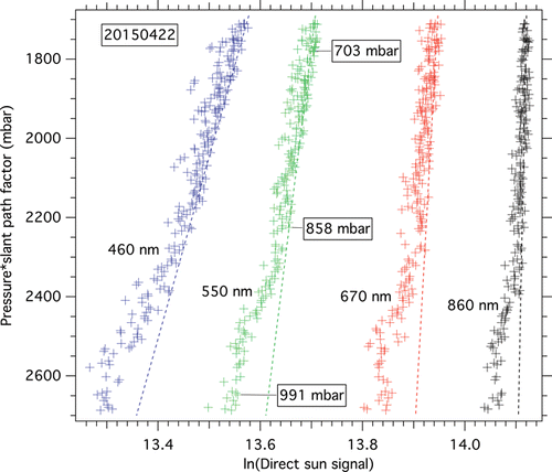
Most of the scatter of points in Figure 4 is because the attitude compensation could not keep the slit perfectly centered on the sun as the Manta UAS rolled up to ±20°. There was less scatter when the photometer was not tilted. An off-center slit slightly changes the amount of scattered sky light, but there may be some additional noise from non-uniform response inside the photometer optics. About 20% of the azimuth scans have been eliminated from the figure because of obvious clipping of the sun. Additional points were removed from the 860-nm channel, apparently because its slit was misaligned compared with other three channels.

The layer aerosol optical depth on the slant path is the difference between the sun signal and Rayleigh scattering (dashed lines). For the green channel, this is about 0.08 between the surface and the top of the profile. The aerosol optical depth is the slant value divided by the airmass factor, which was about 2.7. Therefore, the green layer aerosol optical depth was about 0.03. This small optical depth is easily discernable. Judging from the scatter in Figure 4, the detection limit is better than 0.01, comparable with a newly calibrated AERONET sun photometer (Holben et al. 1998). On a more stable platform, the detection limit could be much better. One reason for the good detection limit is that the absolute sensitivity of the miniature sun photometer described here only has to be stable for about an hour during a vertical profile rather than for one or two years between calibrations of a ground-based photometer.

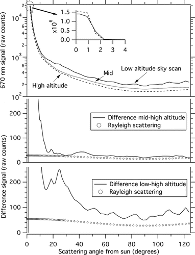
The sky scans (Figure 5) show the sky getting brighter with increasing atmospheric path length. The residual difference in sky brightness after the Rayleigh scattering has been accounted for is mostly forward scattering as expected for aerosols. At this point, we have not quantitatively analyzed the noise in the sky brightness. The general pattern of more aerosol scattering at small angles was reproducible on successive scans and on each side of the sun but smaller features, such as the peak near 25°, were not. The flight was near the boundary between ocean and glaciers, so there was extreme variability in surface albedo.

Figure 5. Scans of sky radiance. The upper portion of the graph shows the average of three scans each from near the top, middle, and bottom of the altitude range (at 703-, 858-, and 991-mbar tags shown in Figure 4). The inset shows how the direct sun signal is larger at high altitude whereas the sky signal is larger at lower altitude. The lower portions of the graph show the difference between the traces and the calculated Rayleigh scattering contribution. The red aerosol optical depth was about 0.03.

Calibration

A short calibration was carried out at the NASA Goddard Space Flight Center (GSFC). A miniSASP was operated on the roof calibration platform for a portion of a day along with a reference AERONET photometer there (Figure 6). The reference photometers are recalibrated every three to six months at Mauna Loa to an AOD uncertainty of 0.002 to 0.005 (Eck et al. 1999). The curves are the miniSASP data at all four wavelengths. The AERONET aerosol optical depths (http://aeronet.gsfc.nasa.gov/new_web/data.html, accessed June 2015) for GSFC were interpolated to miniSASP wavelengths. The circles are the sum of the interpolated aerosol optical depths plus Rayleigh scattering, multiplied by the air mass factor. For reference, the red and blue aerosol optical depths were about 0.03 and 0.06 respectively. The miniSASP reproduces the change in aerosol optical depth before and after noon (about 0.02 in the blue). The green channel does not perform, as well as the other three wavelengths. We believe this is because of a neutral density filter that was put in the green channel in this instrument to avoid saturating the digitizer in the brightest conditions. It appears that this filter took over an hour to stabilize, perhaps because of moisture. A better neutral density filter or perhaps a narrower bandpass filter will be used if future photometers need to attenuate the green channel.

Figure 6. Roof top comparison to the AERONET sunphotometer at NASA Goddard Space Flight Center. The miniSASP data have been scaled with a single sensitivity factor for each channel. The symbol size used for the AERONET data is about 0.01 in AOD units at a solar zenith angle of about 60°. The air mass factor is just 1/cos (solar zenith). Sharp drops in all channels are due to clouds. See text for a discussion of green channel.

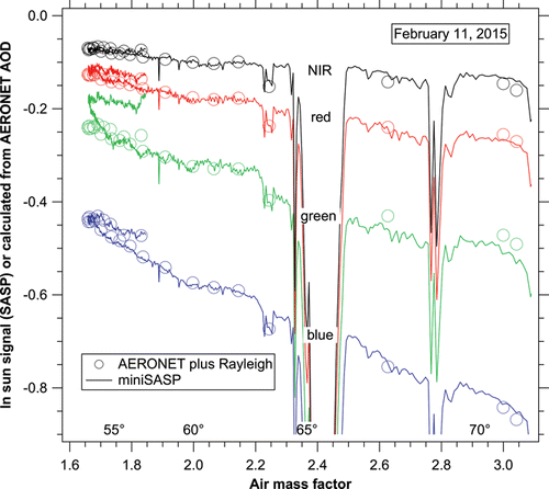
Figure 6 shows excellent agreement throughout a day with a reference sun photometer. Checking long-term stability would take additional comparisons, although the main goal of the miniSASP photometer is short-term profiles. It was not possible to compare the almucantar scans with AERONET because most of the scans have only a few angles, probably due to scattered clouds. The rooftop comparison was run only for one day.

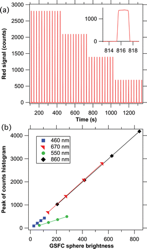
Figure 7 shows data from miniSASP pointed at the 1-m GSFC calibration sphere, which is equipped with lamps traceable to an NIST standard. Every 30 s, the sphere came in view and the lamps in the sphere were cycled through four brightness settings (http://spectral.gsfc.nasa.gov/docs/Cal/Slick/2015/). The photodiode responses are extremely linear: r² values for linear fits are well above 0.99 for all four channels.

Figure 7. Sphere calibration at NASA GSFC. (a) Raw data from the red channel for calibration. The inset shows the photometer view rotating once past the integrating sphere. For each lamp brightness, a histogram was constructed of the signal for each color. The maximum of the histogram was used as the channel response for each lamp setting. (b) The linear response of all four channels. The green channel intentionally has a lower sensitivity to avoid saturation near the peak of the solar spectrum.

Conclusions

We have described a four-color miniature sun photometer suitable for vertical profiles of aerosol optical depth within layers from light platforms, such as small balloons, and UASs. Preliminary flight data show a detection limit better than 0.01 in aerosol optical depth for a vertical profile through the bottom few kilometers of the atmosphere.

Funding

This work was funded by an internal NOAA seed money grant as well as NOAA base and climate funding. Funding for the flight time was provided by the Gordon and Betty Moore Foundation.

References

- Bates, T. S., Quinn, P. K., Johnson, J. E., Corless, A., Brechtel, F. J., Stalin, S. E., Meinig, C., and Burkhart, J. F. (2013). Measurements of Atmospheric Aerosol Vertical Distributions above Svalbard, Norway Using Unmanned Aerial Systems (UAS). Atmos. Meas. Tech., 6:2115–2120.
- Dunagan, S. E., Johnson, R., Zavaleta, J., Russell, P. B., Schmid, B., Flynn, C., Redemann, J., Shinozuka, Y., Livingston, J., and Segal-Rosenhaimer, M. (2013). Spectrometer for Sky-Scanning Sun-Tracking Atmospheric Research (4STAR): Instrument Technology. Remote Sens., 8:3872–3895.
- Eck, T. F., Holben, B. N., Reid, J. S., Dubovik, O., Smirnov, A., O'Neill, N. T., Slutsker, I., and Kinne, S. (1999). Wavelength Dependence of the Optical Depth of Biomass Burning, Urban, and Desert Dust Aerosols. J. Geophys. Res., 104(D24):31333–31349. doi:10.1029/1999JD900923
- Holben, B. N., Eck, T. F., Slutsker, I., Tanre´, D., Buis, J. P., Setzer, A., Vermote, E., Reagan, J. A., Kaufman, Y. J., Nakajima, T., Lavenu, F., Jankowiak, I., and Smirnov, A. (1998). AERONET – A Federated Instrument Network and Data Archive for Aerosol Characterization. Remote Sens. Environ., 66:1–16.
- Karol, Y., Tanré, D., Goloub, P., Vervaerde, C., Balois, J. Y., Blarel, L., Podvin, T., Mortier, A., and Chaikovsky, A. (2013). Airborne Sun Photometer PLASMA: Concept, Measurements, Comparison of Aerosol Extinction Vertical Profile with Lidar. Atmos. Meas. Tech., 6:2383–2389.
- Kim, S.-W., Yoon, S.-C., Dutton, E. G., Kim, J., Wehrli, C., and Holben, B. N. (2008). Global Surface-Based Sun Photometer Network for Long-Term Observations of Column Aerosol Optical Properties: Intercomparison of Aerosol Optical Depth. Aerosol Sci. Technol., 42:1–9.
- Matsumoto, T., Russell, P., Mina, C., Van Ark, W., and Banta, V. (1987). Airborne Tracking Sunphotometer. J. Atmos. Oceanic Technol., 4:336–339.
- Mims, F. M. III (1992). Sun Photometer with Light-Emitting Diodes as Spectrally Selective Detectors. Appl. Opt., 33:6965–6967.
- Mims, F. M. III (2002). An Inexpensive and Stable LED Sun Photometer for Measuring the Water Vapor Column over South Texas from 1990 to 2001. Geophys. Res. Lett., 29: article 1642. doi:10.1029/2002GL014776.
- Schmid, B., Livingston, J. M., Russell, P. B., Durkee, P. A., Jonsson, H. H., Collins, D. R., Flagan, R. C., Seinfeld, J. H., Gassó, S., Hegg, D. A., Öström, E., Noone, K. J., Welton, E. J., Voss, K. J., Gordon, H. R., Formenti, P., and Andreae, M. O. (2000). Clear-Sky Closure Studies of Lower Tropospheric Aerosol and Water Vapor during ACE-2 Using Airborne Sunphotometer, Airborne In situ, Space-Borne, and Ground-Based Measurements. Tellus B, 52:568–593.