Fast high-resolution nanoDMA measurements with a 25 ms response time electrometer

ABSTRACT

Two fast electrometer circuits (10¹¹ and 10¹² V/A) are installed in a Faraday cage having a relatively small residence time. Removing readily distinguishable occasional spikes, the root mean square (r.m.s.) noise level at 10¹² V/A is 0.11 fA when acquiring data at 1 Hz. This value is close to the expected thermal resistor noise at room temperature (0.09 mV). Both electrometers exhibit a 20 ms flow-related delay, followed by respective half-height rise-times of ∼4 and 25 ms. Fast high-resolution mobility spectra in the 1–2 nm size range are acquired with electrosprayed tetraheptylammonium ions by combining these electrometers with a high-speed DMA. At 10¹² V/A, there is no ion mobility peak distortion when acquiring data with discrete voltage steps and dwelling 100 ms at each voltage. With the 10¹¹ V/A electrometer, the DMA voltage V_DMA is continuously swept up and down over 600 V in a triangular wave, at up to 1200 V/s. A shift ΔV_DMA in the peak center is apparent, with little peak shape distortion. ΔV_DMA is symmetric with respect to up or down sweep, and linear with sweep frequency, corresponding approximately to a pure delay Δt = 25 ms. This peak displacement may be offset by adding the correction ΔV_DMA = Δt (dV_DMA/dt) to the measured peak voltage. Extrapolating the measurements made here over a mobility range Z_max/Z_min of 4 to a much wider mobility range of 300 typical of aerosol studies, we conclude that almost undistorted high-resolution mobility spectra may be acquired in 1.3 s.

Copyright © 2017 American Association for Aerosol Research

EDITOR:

• Jian Wang

1. Introduction

The differential mobility analyzer (DMA) has been one of the most useful tools available to study particles smaller than 100 nm (Knutson and Whitby 1975; Liu and Pui 1974). It is a narrow band filter, which, like the quadrupole mass spectrometer, requires scanning to provide a size (mobility) spectrum. The interest of capturing fast evolving events has therefore stimulated efforts to either minimize the scan time, or to develop non-scanning measurement techniques (Olfert et al. 2008, Wang 2009). Other non-scanning mobility separation instruments with good time resolution are mentioned by Shah and Cocker (2005). Others are commercially available, such as TSI's Fast Mobility Particle Sizer™ Spectrometer Model 3091, Cambustion's DMS500, and the Electrical Aerosol Spectrometer of Tartu University (Tammet, Mirme and Tamm 1998). The scan time in DMA measurements has been traditionally limited primarily by the residence time in the DMA, t_DMA, and the time response of the detector (distribution of residence times t_D in CPCs, or electrical response time of the electrometer amplifier). In TSI's widely used 3085 nanoDMA model, the mean flow velocity at the maximum flow rate of 20 L/min is 38.4 cm/s, resulting (with a 5 cm axial length) in t_DMA = 130 ms. Longer DMAs typically used to classify particles up to 100 nm or beyond often involve residence times larger than 1 s. Traditional aerosol detectors, both condensation particle counters (CPCs) and electrometers, have also had response times of the order of 1 s, so there was for a long time no urgent stimulus to accelerate the response of only one of either the analyzer or the detector. This situation began to change when Stolzenburg and McMurry (1991) developed the first relatively fast CPC, which, however, had limited sensitivity. Another turning point arose when Wang and Flagan (1990) demonstrated the idea of the Scanning Electrical Mobility Spectrometer, enabling inversion of mobility measurements taken at scan rates much faster than previously possible. These novelties stimulated further the development of fast and sensitive CPC detectors, pioneered by Wang et al. (2002), which is currently an active research area (Wehrner et al. 2011). Indeed, instruments responding within 0.1 s are already commercially available (i.e., Brechtel's Mixing Condensation Particle Counter MCPC-Model 1720; TSI model 3788 N-WCPC). A variety of other DMA configurations better suited for fast measurements have been developed, such as Caltech's radial DMA (Brunelli et al. 2009). In the meantime, supercritical DMAs (operating laminarly at Reynolds numbers of many thousands) designed to achieve high-resolution analysis of nanoparticles have also evolved. Coincidentally, their small axial distance L between the inlet and outlet slits and high flow speeds have resulted also in residence times within the DMA typically below 1 ms. This advantage has been exploited in coupling DMAs in tandem with comparably fast quadrupole mass filters (Fernandez de la Mora et al. 2010), in turn relying on the exceedingly fast electron multiplier detectors common in mass spectrometry. But since such rapid and sensitive detectors are lacking at atmospheric pressure, the measurement speed offered in principle by supercritical DMAs has not yet been exploited in earnest to accelerate aerosol size analysis.

It is well known that electrometers based on inverting operational amplifiers may respond very fast. However, the large resistance R determining the voltage to current conversion response (V/I = R) of an operational amplifier also controls the rise time t_e = RC through the effective capacity C between the amplifier output and input. Since this capacity cannot be reduced indefinitely, the higher the amplification, the smaller the speed. And because an electrometer is typically much less sensitive than a CPC, aerosol electrometers have tended to use the highest possible amplifications. With typical parasitic capacities of 1 pF and high amplifications with R∼10¹²Ω, aerosol electrometers have had response times in the range of 1 s. Given this background, we were recently startled to learn that an electrometer circuit developed at the University of Applied Sciences, Windisch (IAST) with R = 10¹²Ω, had a noise level (∼0.13 mV) and a response time (∼100 ms), both some 10 times smaller than traditional aerosol electrometers. The same IAST circuit with a 10¹¹Ω resistor responded in ∼10 ms. The present study accordingly explores the measurement speed advantages offered by combining a supercritical DMA with these two amplifier circuits. The most interesting finding is that, at scanning speeds at which the classification voltage V_p of a monomobile particle is substantially (11%) shifted by a value ΔV_p, the DMA transfer function is simply translated by ΔV_p, and otherwise only very mildly distorted. This voltage displacement is strictly proportional to the scan rate dV/dt, and can as a result be accurately corrected by the software controlling the scan.

2. Experimental methods

2.1. Electrometer

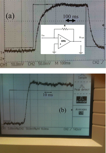
Two amplifier circuits developed at IAST and previously employed in aerosol studies (Fierz et al. 2014) were used. They had V/I responses of 10¹¹ and 10¹² V/A, and will be referred to, respectively, as the fast and the slow electrometer. They are conventional inverting amplifiers, with a schematic given in the inset to Figure 1a. Their key components are the amplifier (LMP7721MA from Texas Instruments) and the 10¹¹ and 10¹²Ω amplifying resistors (SRT resistor technology, models CHS 2512 1T ±10% TCR 500 and CHS 2512 100G ±10% TCR 1000; http://www.srt-restech.de). Each circuit was incorporated into a Faraday cage electrometer where the aerosol was collected in a metallic filter, and the received charge flowed to the input line of the amplifier. The estimated dead volume between the outlet slit of the DMA and the filter surface was 2 cm³, corresponding at 3 L/min to a residence time of 40 ms. The actual residence time was less, perhaps because the gas jet entering the small chamber immediately upstream the collector filter is uniformly sucked into the filter material, not filling the whole chamber with recirculation regions. Considerable effort was devoted to minimize the noise added to the bare amplifier circuit by the mechanical components of the Faraday cage, resulting in an integrated aerosol electrometer now commercialized by SEADM (http://www.seadm.com/products/technological-modules/electrometer/).

Figure 1. Oscilloscope traces for (a) the slow (10¹²Ω) and (b) the fast (10¹¹Ω) electrometers (schematically shown in the inset to (a)), showing a comparable (∼20 ms) initial time delay with no response for both. Half-height rise times are approximately 22 ms and 4 ms.

The static amplification of the electrometer was determined at Yale by applying a known voltage to one end of a 10¹¹Ω resistor. The other end of the resistor was virtually grounded through the input wire of the amplifier, injecting a known current into the circuit. Within the ambiguity in the value of our calibration resistor, the measured transimpedances of 10¹¹ and 1.1 10¹²Ω agreed with the values 10¹¹ and 10¹²Ω provided by the IAST group.

2.2. Electrometer noise and long term drift

A brief study of the noise level and long-term output signal drift was made by acquiring data from the slow (10¹² Ω) electrometer output, with no aerosol input. The signal was sampled at 250 kHz and averaged over 1 s intervals. In order to quantify the drift in the background current, the electrometer output was recorded continuously overnight in the absence of an aerosol, including 100 different series, each containing 250 data points.

2.3. DMA

We relied on a previously described portable cylindrical DMA dubbed the Halfmini, with inner and outer electrode radii R₁ = 4 mm; R₂ = 7 mm, and with axial distance between inlet and outlet slits L = 2 cm (Fernandez de la Mora and Kozlowski 2013). The monodisperse aerosol line going from the outlet slit to the electrometer inlet has an inner diameter of 3 mm and a length of ∼70 mm, with a total dead volume of ∼0.5 cm³. The inlet and outlet flow rates q_i and q_o were approximately matched at 3 L/min. Both were measured with ball flowmeters, one upstream the aerosol generator, the other downstream the electrometer outlet. The sheath gas flow rate Q was not directly measured. It may be determined for this and other cylindrical DMAs from the relation 2πLVZ/Q = ln(R₂/R₁), where V is the voltage at which the transfer function peak appears for a monomobile aerosol with mobility Z. This voltage was 374 V for the tetraheptylammonium ion (Z = 0.97 cm²/V/s), with a corresponding Q = 488 L/min. The sheath gas was taken from the atmosphere (without drying) through a HEPA filter into a vacuum cleaner pump, then injected into the DMA, and finally released back to the atmosphere. Note the important point that the peak shape in a mobility spectrum obtained by scanning the DMA voltage with a monomobile ion is, by definition, identical to the shape of the DMA transfer function.

2.4. Pulsed aerosol generation

In preliminary experiments we selected the most prominent and mobile negative species produced by a Ni-63 beta emitter in air (mobility estimated as 2 cm²/V/s based on the assumption that the ion mobility is close to the polarization limit). The DMA voltage was periodically switched between zero and this V by means of a high voltage switch (PVM-4140 from DEI; <1 μs switching time). The electrometer signal was tracked in an oscilloscope (Tektronix, TDS 210), whose screen was occasionally photographed (Figure 1). Q was not measured in these experiments, but its value was comparable to the 488 L/min used in subsequent experiments with tetraheptylammonium ions. Under these conditions the gas velocity is ∼100 m/s and the residence time of the selected particles in the analyzer is ∼0.2 ms. The residence time within the analyzing region would still be small compared to other delay times in this setup even if Q were decreased tenfold.

Fast mobility spectra were acquired with a digital oscilloscope (Analog Discovery, 100 Ms/s, from Digilent, sampling at 100 MHz and providing an averaged file with 8000 data points). This device also generated a periodic low-voltage triangular wave that was used as the control for a high voltage power supply (Applied Kilovolts, model HP005RAA025, ±5 kV, 2 mA) connected to the inner electrode of the halfmini DMA. This relatively fast power supply is commonly used in quadrupole mass spectrometers and can switch from +5kV to −5 kV in less than 20 ms. One oscilloscope channel read the DMA voltage through a fast high-voltage probe [Tek P5100 100x from Tektronix]. Another oscilloscope channel read the electrometer output. The test aerosol was dominated by the tetraheptylammonium ion (THA⁺), generated by electrospraying in air an unusually dilute solution of tetraheptylammonium bromide in ethanol, such that the dimer ion was far less abundant than the monomer. We chose a triangular wave to determine the shift in peak position in positive and negative sweep. It went from 0 V to approximately −600 V and back to zero at a frequency f, so that the sweep rate was[1]

These continuous mobility spectra were taken only with the fast electrometer.

3. Results

3.1. Electrometer noise and drift

Figure 2 (gray line) shows a typical electrometer response. The average background signal is approximately 5 mV, as a zero-correction was not applied. The r.m.s. variation with respect to the mean is σ = 0.236 mV. The data series represented by crosses in Figure 2 removes (manually) 5 well-defined outlier points, which (i) are always isolated (the data point before and after the outlier always fall either above or below the outlier point) and (ii) they depart from the mean by far more than would be allowed (with a realistic probability) by a Gaussian distribution with the given σ. Given these singular distinguishing features, a visual selection of outliers seems natural enough. A more rigorous justification of this removal will be provided in Section 3.2. Removing these 5 points results in an r.m.s. noise of about 0.12 mV. Nine such data series were analyzed, and found to have quite consistent σ values in the range 0.119–0.136 mV when eliminating the events. The number of events in each of these nine series varied from 4 to 20.

Figure 2. Blank data series for the 10¹²Ω electrometer containing 251 output data, each accumulating signal for 1 s. The full series (gray lines) includes five isolated outlier points, whose removal (crosses) decreases the r.m.s. noise from 0.236 mV to 0.135 mV.

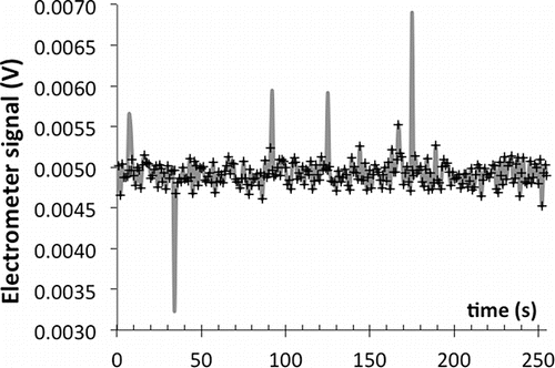
Given that the electrometer is subject at least to the thermal resistor or Johnson noise (Nyquist 1928), it is natural to use as reference its standard deviationwhere k_B is Boltzmann's constant, T the absolute temperature, R the resistance of the amplifying resistor and Δf the bandwidth. For the original measurement at 250 kHz the bandwidth is half of this frequency. Since the signal is accumulated for 1 s, 250,000 samples are taken, so the standard deviation is divided by (250,000)^1/2. The result is equivalent to using Δf = ½ Hz, which, for a 10¹²Ω resistor at 23°C yields σ_J = 0.0904 mV. Since this minimal noise reference is close to the noise of our event-corrected data, one is forced to interpret most of the event-free part of the observed background as thermal noise. The outlier points have an amplitude of ∼1 fA (∼1 mV), comparable to that of other aerosol electrometers, so it is reasonable to assume that both have the same unclear but evidently non-thermal origin. What is special here is that the small frequency of the events enables their isolation and removal, effectively reducing the noise level almost to the thermal value. Note finally that, at a sample flow rate of 3 L/min, the observed noise of 0.135 mV corresponds to 16 singly charged particles/cm³.

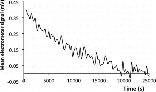
The mean electrometer signal for 100 series each of 251 data (uncorrected for the events) is shown in Figure 3 as a function of the mean time for the series, providing a measure of the drift level of 0.057 mV/h over a 7-h period. For typical experiments taking minutes, the zero drift is insignificant even at the scale of a 0.1 mV noise. Noise and drift become comparable for measurements taking one hour, while the drift may dominate for long-term measurements. In this case the aerosol needs to be briefly cancelled (say for 10 s once every 20 min) to record the temporal evolution of the baseline. If the instrument is monitoring mobility spectra and every voltage scan dwells briefly at V_DMA = 0, each spectrum would automatically include information of its own zero.

Figure 3. Long term output drift for the slow (10¹²Ω) electrometer.

3.2. Statistical analysis of the electrometer noise

Knowing that most data points result from resistor noise and therefore have a Gaussian distribution, we may now compute the probability that a suspected outlier may actually be a genuine part of this Gaussian distribution. The cumulative distribution for a large number N of values x_i of a certain variable x having Gaussian statistics with standard deviation σ and mean x_o is given in terms of the error function Erf as:[2] where NP(x) gives the number of data with values x_i larger than x-x_o. Two practical advantages of working with the cumulative distributions are that (i) it gives directly the actual integer number of measurements (ordinary data and outlier data), and (ii) the data are only divided into two rather than many bins, providing less noisy statistical information (by avoiding the known inaccuracy of computing derivatives of experimental data). Taking σ = 0.12 mV (0.12 fA), the probabilities P in Equation (2[2] ) for one datum falling 0.5 and 0.4 mV below the mean are, respectively, 1.54543 10⁻⁵ and 4.2906 10⁻⁴. In a sample of 251 data this corresponds to 0.0039563 and 0.109839 events, respectively. It is accordingly most unlikely that a single datum in such a Gaussian distribution will deviate 0.4 mV from the mean. The fact that 5 data in a group of 251 data deviate from the mean by more than 0.5 mV (two of them by more than 1.5 mV) shows without any doubt that these data are not the result of thermal noise, but of some other far more energetic cause. In order to confirm more quantitatively this conclusion, we have taken two additional data sets with many more samples: one with 1800 data, another with 57,600 data. The small temporal drift of the mean in a series of 1800 data was compensated by removing the 9 outliers points departing by more than 0.4 mV from the mean. This excised temporal series was fitted by linear regression, and the fit was subtracted from all the data (including the original outliers) to yield a drift-free series with zero mean. The same procedure was used for the larger series. However, because the evolution of the larger series over such a long time was not as well represented by a straight line as for the shorter series, a mean versus time curve <x(t)> was alternatively determined manually from the dense cloud of data points represented versus t, fitted, and subtracted from the raw data series to produce an alternative drift-free series with zero mean. These two drift correction methods gave almost identical distributions for the 57,600 data series.

Both series were statistically analyzed while removing a variable number p of events. The analysis involves simply putting the data points in a column, ordering them by increasing values, and representing the normalized column number i(x_i)/(N-p) versus the value x_i of each of the ordered noise signals. This representation provides directly a cumulative distribution. Ordering the data was achieved with the Sort command in Excel (for the 1880 data set) or Mathematica (for the 57,600 data set). Events may be readily removed by eliminating an increasing number of data at the top and bottom of the column, where outliers are ordered by their level of departure from the mean.

Figure 4a shows the cumulative distributions for the set of 1800 noise data, together with a best fit to Equation (2[2] ). Using σ = 0.111 mV the fit is excellent in the left part of the curve, while the right part is similarly well fitted with σ = 0.117 mV. Aside from this slight 0.006 mV asymmetry (perhaps due to negative events of low signal) the agreement with theory is excellent. Figure 4b uses a logarithmic scale to display anomalies on the tails of the distribution. The right portion of the curve represents 1-P rather than P, in order to capture anomalies in the right tail of the distribution. The + symbols corresponding to p = 0 give an almost perfect Gaussian behavior on the right tail, showing that there are no outliers on the positive side of the distribution. The disagreement is substantial on the left tail, but becomes excellent when 9 outlier points are removed. Removing either 8 or 10 outliers results in a clear departure from the theory. Most of the noise observed is therefore thermal, with the 9 outliers having an evidently non-thermal source. In this example, the correct criterion for event suppression is elimination of all data whose absolute value exceeds the mean (of the excised series) by 0.4 mV.

Figure 4. Cumulative distributions for a series of 1800 1-s noise data (corrected for drift and with mean value shifted to the origin) from the 10¹² Ω electrometer. (a) Linear scale representation with σ = 0.111 mV in the fit to Equation (2[2] ). (b) Logarithmic scale for a variable number p (0, 7, 8, 9, 10, as given in the legend) of data with large negative signal removed from the series. The right portion of the curve represents 1-P in order to capture anomalies in the right tail of the distribution.

Whatever the source of the 9 data with non-thermal noise, its distribution shows a slow decay with the noise level V, apparently algebraic, which enables a few outlier points to dominate completely the distribution of large negative noise. The distribution of outliers is best analyzed with the 57,600 data set, containing over 500 events. This large number permits also probing deeper into the tail of the distribution, revealing a non-Gaussian behavior also on the right tail. In this case neither the positive nor the negative non-Gaussian tails may be removed by suppressing data with large signals no matter how large their number p (Figure 5b). Plotting the logarithm of the absolute value of the noise signal versus the logarithm of the normalized number of events i/(N-p) yields straight lines, confirming that the cumulative distribution of events decays indeed algebraically, P(x) ∼ x^−s as |x|>>σ (Figure 6). A similar scaling with s ∼ −2 is found also for the negative outliers in the 1800 data set, though with the lesser confidence offered by only 9 outlier points. Normalizing the two tails by the total number N of data in the distribution results in a considerably more intense tail of outliers in the 1800 data set than in the 57,600 data set, suggesting that the number of outliers depends on uncontrolled circumstances.

Figure 5. Cumulative distributions P(noise) for the 57,600 data set. (a) Linear representation with the data in Gray. (b) Natural log₁₀ representation showing non-Gaussian behaviour on the tails, irrespective of the number p of outlier points suppressed (p = 0, 25, 50, 75 on the right; p = 0, 100, 200, 300, 375 on the left). (c) Representation of the distribution of outliers as log₁₀(i) versus log₁₀(|noise|), with straight lines showing algebraic decays i∼|noise|^s, with s = −2.15 on the left and −3.33 on the right tail.

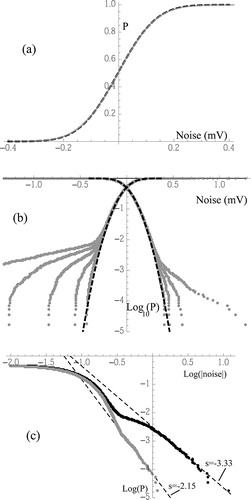
In conclusion, statistical analysis of the noise confirms its dominantly thermal origin, both through its Gaussian distribution and through its standard deviation of about 0.11 mV. The few outliers arising have an evidently super-thermal origin (one event at 11.9 mV), whose slow algebraic decay permits rare events with large amplitudes. The largest among these events can easily be removed without loss of information by eliminating all data exceeding the mean (or the two neighboring data points) by more than ±0.4 mV. Some non-thermal contributions to the noise probably arise below 0.4 mV and cannot be so easily removed. This possibility is indicated by asymmetries observed between the positive and the negative pieces of the distribution within the thermal range of noise amplitudes below 0.4 mV. However, the small magnitude of these asymmetries (0.006 mV) show that the non-removable fraction of outliers has no significant effect on the overall noise.

3.3. Intrinsic response time of the DMA-electrometer system

Figure 1 shows oscilloscope traces resulting from pulsing the aerosol with the high voltage switch. Two characteristic times involved are of interest. There is a first interval Δt₁ before the signal begins to rise, to be referred to as the delay, and a second interval Δt₂ taken by the signal to rise from zero to 50%, to be referred to as the risetime. Measured half-height risetimes are approximately 22 ms and 4 ms, corresponding approximately to the expected decay e^−t/RC, with RC products of ∼32 ms and ∼5.9 ms. The circuit includes no capacitor, so the corresponding C values of 0.032 pF and 0.059 pF are purely parasitic and substantially smaller than 1 pF. The delay is similar for both electrometers, suggesting that it is due to the finite response time in either the analyzing region of the DMA or on the outlet tubes. It cannot be due to time lag in the voltage power supply because the high voltage switch responds in sub-μs times. The delay cannot be associated to the analyzer, whose residence time was previously estimated as 0.2 ms. The explanation for the initial delay appears to be more complex than just the residence time in the outlet tubes, because a few preliminary measurements indicated that the dependence of Δt₁ on sample flow rate is not linear. The issue would be worth pursuing if one sought response times smaller than 20 ms, but was beyond this preliminary exploration.

3.4. Fast mobility spectra measurements

Figure 6a shows the oscilloscope time traces V(t) and I(t) for f = 0.6 Hz. The subsequent panes (b-f) show measured mobility spectra I(V) acquired at increasing sweep frequencies, displaying an increasing displacement of the peak positions for the up and down sweeps, while the peaks remain narrow even at the highest frequency. The upscan (dashed line) and downscan peaks (continuous line) are shifted respectively to the left and the to the right. The corresponding peak voltages are plotted in Figure 7 as a function of sweep frequency f, showing a linear increase of V with f, almost exactly symmetric in the up and down scans

Figure 6. Mobility spectra dominated by the THA⁺ peak, taken with the fast electrometer and an oscilloscope using a triangular wave going back and forth from 0 to −600 Volt. (a) Time traces for the applied voltage and the measured monodisperse particle current. (b) to (f) Measured DMA current versus applied voltage at the indicated sweep frequencies. The upscan peak (dashed line) is shifted to the left and the downscan peak (continuous line) to the right. The inset to (f) shows the 60 Hz noise ripple in the raw time trace.

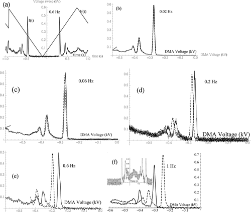
Figure 7. Shift of the peak voltage for the THA⁺ ion as a function of sweep frequency f, with almost symmetrical displacements in the up and down sweeps.

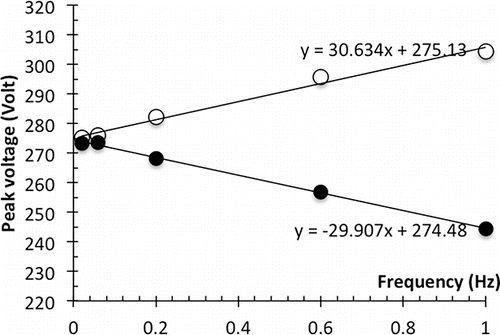
At f = 1 Hz, dV/dt = 1200V/s, while the voltage shift measured experimentally is 30.3 V, indicating that the response time of the electrometer is 25 ms. This is reasonable, as the initial delay for any response observed in Figure 1 was 20 ms, and the time for rise to half height was 4 ms.

Note in Figures 6d an increase in noise at 0.2 Hz. This is artificially due to poor shielding of the connection between the electrometer output and the oscilloscope, as evident from the dominant 60 Hz component of the noise (inset to Figure 6f). At low sweep frequencies the original noise was greatly reduced by averaging 10 neighboring data points. At higher frequencies this approach was ineffective because the 10 points used for averaging did no longer span a full 60 Hz period, while averaging over more points degraded resolution. In Figures 6e and f (0.6 and 1 Hz), the background noise was greatly reduced by subtracting from the measured signal pure 60 Hz sine waves with optimally selected amplitudes and phases.

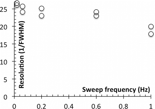
Although less prominent than the peak displacement, a modest increase of peak width with frequency is also noticeable, especially as a tail appearing at the highest frequencies on the side towards which the peak center is displaced. This widening effect is quantified in Figure 8, based on the inverse relative full peak width at half maximum (FWHM). Because the relatively large sample flow rate used (q = 3 L/min) degrades DMA performance, 1/FWHM is limited to 27 even at zero frequency. The two data points shown at each frequency (corresponding to the up and down sweep) give a measure of the relatively large error involved in the measurement of FWHM, irrespective of the sweep direction.

Figure 8. Loss of resolution on the THA+ peak at increasing sweep frequency.

In conclusion, the fast electrometer may take high resolution mobility spectra in time periods in the range of 1 s, with little widening of the DMA response function, though with the need to correct the peak position according to a delay time of 25 ms, by substituting the time-shifted voltage (3[3] ) in lieu of the actual DMA voltage:[3]

Note that most of the delay observed corresponds to the initial 20 ms time lag rather than the 4 ms half rise time of the amplifier circuit. As already noted, this lag is the same for the circuit with a 10¹²Ω resistor, so an even faster electrometer with less amplification would not help overall measurement speed unless the voltage shift correction is made with considerable accuracy. For further improvements one would need to understand and overcome this initial time lag, probably related to the finite gas volume between the analyzer and the detector. This effort would be very worthy, as it could accelerate the measurement 5-fold without changes in the electronic circuit.

4. Discussion

Comparison between prior related efforts and our own method of correcting mobility spectra acquired at high frequency is of some interest. The difficulties involved and the various approaches used to overcome them are reviewed by Flagan (2014). In their scanning electrical mobility spectrometer, assuming an ideal DMA and detector behavior, they can unambiguously relate highly distorted fast mobility spectra to the original mobility spectrum. As often happens with inversion approaches, non-idealities in the DMA response and the compounded effect of complex residence time distributions in the detector set limits on the faithfulness of the recovered spectra. For this reason, really fast scans (a few seconds) had to wait for the development of fast detectors (Wang et al. 2002), whose commercial implementation has only taken place recently. For instance, using TSI's 3788 CPC having a response time of 0.1 s, Tröstl et al. (2015) report the acquisition of spectra in the 1–20 nm diameter range (Z_max/Z_min = 380) with a test aerosol spanning a moderately narrow range of diameters from 6 to 8 nm. Their scans took as little as 3 s, with the 5 s scan showing only a slight distortion, and the 10 s scan being virtually indistinguishable from the 60 s scan. Shah and Cocker (2005) combined Caltech's fast CPC and fast radial DMA already mentioned. Their Figure 2 shows mobility spectra from 5 to 100 nm (Z_max/Z_min ∼306), including a monodisperse aerosol with a size distribution spanning particle diameters from 55 nm to 80 nm. Their 5 s scanshows a 27% shift (from 70 to 80 nm) of the low-mobility tail, with very little shift of the high mobility tail. Their 10 s scan shows a relatively slight distortion at high mobility, with no distortion at low mobility with respect to the 30 s scan (in turn almost identical to the 60 s scan). The relatively slight transfer function distortion in the10 s scan is not so slight when examined at the resolving powers offered by our measurement system. The base of their triangular size distribution (55–80 nm) spans a mobility ratio of 1.97, with a corresponding ratio of 1.4 at half the maximum height. Seen at the scale of our almost 10 times narrower mobility peak, their 10 s scan would appear as considerably distorted (Collins et al. 2004).

In our work, Z_max/Z_min has been limited to just 4. In order to make a quantitative comparison with prior reports covering a much wider mobility ratio, we adopt the favorable exponential scan V(t) = V_oe^−t/τ of the Scanning Electrical Mobility Spectrometer. We choose the decay time τ to match the conditions of the 1 Hz measurement of tetraheptylammonium shown in Figure 6f. Since dV/dt = 1200 V/s, and the peak is centered at V = 275 volt, the time constant of the exponential scan is τ =V/(dV/dt) = 0.23 s. Our pure delay inversion (3[3] ) implies in this case simple substitution of V by V(1+Δt/τ), with Δt/τ = 0.109. The times τln(Z_max/Z_min) required for full scans would then be 1.31 s and 1.36 s for Z_max/Z_min of 306 and 380. At this scanning speed, prior studies have observed substantial spectral deformation, while we see little degradation even on a substantially narrower peak.

The extrapolation made from the modest mobility ratio actually tested in our experiments to the wider ranges usually covered in aerosol measurements will now be critically evaluated. The electrometer delay is Z-independent, so covering an extended Z range would not change the quality of its temporal response. The DMA transfer function at given flow rates (q, Q) depends only on ZV, so our extrapolation to smaller Zs is limited only by the maximum voltage of our DMA (5 kV). The mobility range at the flow rate of sheath gas used to obtain the data of Figure 6 going to 600 V may only be increased by a factor 5/0.6, to reach Z_max/Z_min = 33. Achieving a mobility range of 300 would require operating the halfmini DMA at 54.2 L/min. A first consequence of this 9-fold flow reduction would be to increase the drift time in the analyzer from 0.2 ms to 1.8 ms, resulting in a slightly increased total delay of 26.6 ms rather than 25 ms. This change would be irrelevant in a DMA of high resolving power, since the drift time delay is not only relatively short, but is also nearly the same for all the transmitted ions. Therefore, the spectral distortion would still be close to a pure delay. A second effect of reducing Q would be to substantially increase Brownian diffusion at particle diameters below 2 nm. However, the resulting broader transfer function would still represent the genuine DMA response, irrespective of whether the scanning is fast or slow. The reason for this is that Brownian motion has a much weaker effect on the motion along the direction of the particle motion (hence the flight time) than on the lateral spreading of the cloud. These considerations highlight the strong coupling between scan speed and DMA resolution. If the response of the fast CPCs previously discussed matched that of our electrometer, the distortions found by Tröstl et al. (2015) and Shah and Cocker (2005) in their fastest scans would have to be due to imperfections in the DMA flows. Indeed, a broad transfer function associated to flow or geometrical DMA imperfections results inevitably in a distribution of drift times in the analyzer. And if the drift time is not small, this yields fast-scan distortions more complex than a simple translation in time. Conversely, a narrow transfer function is associated to a narrow distribution of flight times, with a transfer function distortion closer to a pure delay. Furthermore, as long as the pair (q, Q) is fixed during a voltage scan and the transfer function remains narrow over the whole Z range, the magnitude of the flight time delay is fixed for all mobilities.

Given that fast undistorted response function measurements must rely on a fast detector as well as a DMA of good resolving power, it is clear that future fast DMA scanning efforts should pay increased attention to the resolving power. Our Halfmini DMAs is evidently not unaffected by this requirement, as current m-series models show substantial non-idealities at q/Q ratios larger than 2–3%, limiting how much Q may be reduced and therefore limiting the mobility range that may be covered with near ideal response. Although these non-idealities have been recently overcome with a new version of the instrument (p series; Fernandez de la Mora 2017), the effect of this improvement to achieve fast mobility scans at 20–30 nm remains to be demonstrated. Therefore, the known resolution limitations of the current Halfmini DMA call for a revision of our preceding extrapolations. On the assumption that the DMA response remains excellent up to q/Q = 3%, at our sample flow rate of 3 L/min, the sheath gas flow rate may be reduced down to 100 L/min. An expanded mobility range Z_max/Z_min = 33*4.88 = 161 could then be covered with near ideal DMA response, with small expected peak shape distortions comparable to those demonstrated in Figure 6. Doubling this mobility range would result in a resolving power about half the ideal Knutsen–Whitby value for non-diffusing particles (FWHM∼2q/Q), which would still be better than in the studies of Tröstl et al. (2015) and Shah and Cocker (2005).

In conclusion, over the limited mobility range over which the halfmini DMA offers good performance, its combination with a fast detector permits making mobility scans considerably faster and better resolved than previously observed. This favorable size range does not yet extend to 20–30 nm.

5. Conclusions

1. Two inverting amplifier circuits developed at IAST with parasitic capacities much smaller than in prior aerosol electrometers have been installed in two Faraday cage electrometers of small volume, which maintain the fast response and low noise of the bare circuits.

2. The fast circuit having an amplification of 10¹¹ V/A was used as a detector for a half-mini DMA, and the combination was tested at scan speeds up to dlnV/dt = 4.3 s⁻¹. The monomobile ion standards used as test aerosol provide directly the width of the transfer function. The highest scan speeds resulted in a relatively modest transfer function distortion, with a substantial (11%) shift in peak position that could be corrected in terms of a pure shift with a time delay of 25 ms.

3. Extrapolation of the modest mobility range covered in actual experiments here to the range Z_max/Z_min∼300 typical of prior fast DMA scan studies shows that the current setup yields full scans in 1.3 s with considerably less distortion of a narrow aerosol standard, than previously observed with much wider aerosol standards.

4. Given that the speed of response of previously tested fast CPCs appears to be comparable to that of our fast electrometer, we argue that the advantage observed in terms of peak fidelity and scan speed results not only from the fast response of the Half-mini DMA, but also from its high resolution.

Conflict of interest

Following Yale rules, Juan Fernandez de la Mora declares that he has an interest in the Company SEADM commercializing the DMA and electrometers used in this study.

Acknowledgments

Our special thanks go to Mr. Peter Steigmeier (IAST) for developing the two amplifier circuits tested, and to Prof. Roman Kuc for his input on the magnitude of the resistor noise. We are grateful to SEADM for funding various aspects of this study, and to Irene Carnicero (SEADM) for her contributions to the electrometer design.

References

- Brunelli, N. A., Flagan, R. C., and Giapis, K. P. (2009). Radial Differential Mobility Analyzer for One Nanometer Particle Classification. Aerosol Sci. Technol., 43:53–59.
- Collins, D. R., Cocker, D. R., Flagan, R.C., and Seinfeld, J.H. (2004). The Scanning DMA Transfer Function. Aerosol Sci. Technol., 38:833–850.
- Fernández de la Mora, J., Casado, A., and Fernández de la Mora, G. (2010). Method to Accurately Discriminate Gas Phase Ions with Several Filtering Devices in Tandem.US patents 7, 855: 360.
- Fernandez de la Mora, J., and Kozlowski, J. (2013). Hand-Held Differential Mobility Analyzers of High Resolution for 1–30 nm Particles: Design and Fabrication Considerations. J. Aerosol Sci. (57):45–53.
- Fernandez de la Mora, J. (2017). Expanded Size Range of High-Resolution NanoDMAs by Improving the Sample Flow Injection at the Aerosol Inlet Slit. submitted to J. Aerosol Sci., 9 December 2016.
- Fierz, M., Meier, D., Steigmeier, H., and Burtscher, P. (2014). Aerosol Measurement by Induced Currents. Aerosol Sci. Technol., 48(4):350–357.
- Flagan, R.C. (2014). Continuous-Flow Differential Mobility Analysis of Nanoparticles and Biomolecules. Annu. Rev. Chem. Biomol. Eng., 5:255–279.
- Knutson, E.O., and Whitby, K.T. (1975). Aerosol Classification by Electric Mobility: Apparatus, Theory and Applications. J. Aerosol Sci., 6:443–451.
- Liu, B.Y.H., and Pui, D.Y.H. (1974). Submicron Aerosol Standard and Primary, Absolute Calibration of Condensation Nuclei Counter. J. Coll. Interf. Sci., 47:155–171.
- Nyquist, H. (1928). Thermal Agitation of Electric Charge in Conductors. Phys. Rev., 32:110–113.
- Olfert, J. S., Kulkarni, P., and Wang, J. (2008). Measuring Aerosol Size Distributions with the Fast Integrated Mobility Spectrometer. Aerosol Sci., 39:940–956.
- Shah, S. D., and Cocker, D. R. (2005). A Fast Scanning Mobility Particle Spectrometer for Monitoring Transient Particle Size Distributions. Aerosol Sci. Technol., 39(6):519–526.
- Stolzenburg, M. R., and McMurry, P. H. (1991). An Ultrafine Aerosol Condensation Nucleus Counter. Aerosol Sci. Technol., 14(1):48–65.
- Tammet, H., Mirme, , and Tamm, E. (1998). Electrical Aerosol Spectrometer of Tartu University. J. Aerosol Sci., 29:S427–S428.
- Tröstl, J., Tritscher, T., Bischof, O. F., Horn, H.G., Krinke, Th., Baltensperger, U., and Gysel, M. (2015). Fast and Precise Measurement in the sub-20 nm Size Range Using a Scanning Mobility Particle Sizer. J. Aerosol Sci., 87:75–87.
- Wang, S. C., and Flagan, R. C. (1990). Scanning Electrical Mobility Spectrometer. Aerosol Science and Technology, 13:230–240.
- Wang, J., McNeill, V. F., Collins, D. R., and Flagan, R. C. (2002). Fast Mixing Condensation Nucleus Counter: Application to Rapid Scanning Differential Mobility Analyzer Measurements. Aerosol Sci. Technol., 36(6):678–689.
- Wang, J. (2009). A Fast Integrated Mobility Spectrometer with Wide Dynamic Size Range: Theoretical Analysis and Numerical Simulation. J. Aerosol Sci., 40(10):890–906.
- Wehner, B., Siebert, H., Hermann, M., Ditas, F., and Wiedensohler, A. (2011). Characterisation of a new Fast CPC and its application for atmospheric particle measurements. Atmos. Meas. Tech., 4:823–833.