Mass accommodation coefficients of fresh and aged biomass-burning emissions

ABSTRACT

Most chemical transport models treat the partitioning of semi-volatile organic compounds (SVOCs) with the assumption of instantaneous thermodynamic equilibrium. However, the mass accommodation coefficients, α, of biomass-burning organic aerosol (BBOA) are largely unconstrained. During the FLAME-IV campaign, we thermally perturbed aged and fresh BBOA with a variable residence time thermodenuder and measured the resulting change in particle mass concentration to restore equilibrium. We used this equilibration profile to retrieve an effective α for components of BBOA that dictated this profile and found that the mass accommodation coefficients lie within the range 0.1 ≪ α ⩽ 1. A simple plume dilution model shows a maximum of only a 7% difference between a dynamical and an instantaneous equilibrium partitioning model using our best-estimate value for α. This supports continued use of the equilibrium assumption to treat partitioning of biomass-burning emissions in chemical-transport models.

Copyright © 2018 American Association for Aerosol Research

EDITOR:

• Ilona Riipinen

1. Introduction

Airborne particulate matter affects human health and climate. Tens of thousands of people die every year in the United States; globally, several million deaths are linked to air pollution (Nel 2005; Pope III and Dockery 2006). Atmospheric aerosols also absorb and scatter solar radiation, altering Earth's radiative balance (direct effect), and can also affect cloud lifetimes and reflectivity (indirect effect) through serving as cloud condensation nuclei (CCN) (Solomon 2007). The extent to which atmospheric particles affect air quality and the climate depends on, among other factors, their atmospheric loading. This in turn is dictated in part by how the semi-volatile components partition between the particle and gas phases (Donahue et al. 2006). For example, in order to act as CCN, atmospheric particles which are freshly formed from nucleation need to grow to about 50–100 nm. The growth rate therefore actively affects the climate relevance of atmospheric particles (Vehkamäki and Riipinen 2012).

A large fraction (20–90%) of atmospheric particulate matter is comprised of organic species (Jimenez et al. 2009), a significant portion of which is semi-volatile (Robinson et al. 2007; Seinfeld and Pandis 2016). The volatility of organic aerosols (OA) is an important physical property as it determines the phase partitioning and chemical transformations that the OA undergoes (Donahue et al. 2006; Jimenez et al. 2009). Equilibrium partitioning theory (Pankow 1994; Donahue et al. 2006) describes the partitioning between the gas and aerosol phases at equilibrium, the time scale of which is governed primarily by the kinetic properties of the aerosol. This includes the mass accommodation coefficient α, defined here as the ratio of the molecular flux to/from the particles to the maximum flux predicted by kinetic theory (Davis 2006; Saleh et al. 2013). The mass accommodation coefficient is in general poorly constrained. Based on the above definition, an α of unity indicates no condensed phase mass transfer limitations. More specifically, any condensed phase limitations, not explicitly accounted for, will manifest as α less than unity.

Most chemical transport models (CTMs) assume that partitioning kinetics are much faster for sub-micron aerosols than atmospheric processes. This justifies treating atmospheric aerosols as being always at thermodynamic equilibrium, and using equilibrium partitioning theory to portray the gas-particle partitioning of SVOCs. The validity of this assumption for secondary organic aerosol (SOA) is under debate. While some experimental studies support the equilibrium assumption (Jimenez et al. 2009; Saleh et al. 2013; Yatavelli et al. 2014; Liu et al. 2016; Ye et al. 2016), others have indicated that SOA can exist in a highly viscous or glassy state (Vaden et al. 2011; Koop et al. 2011; Renbaum-Wolff et al. 2013) which introduces significant kinetic limitations (α ≪ 1). Diffusion of molecules in this glassy matrix is thought to be very slow, which increases time scales enough to prevent SOA from reaching phase equilibrium at atmospherically relevant time scales (Shiraiwa et al. 2011; Vaden et al. 2011).

The studies cited above which have investigated the effect of diffusion limitations on OA equilibration time scales have been focused on biogenic SOA (mostly α-pinene SOA). In this study, we focus on fresh and photo-chemically aged biomass-burning OA (i.e., including SOA). Biomass burning is a globally important source of OA; it contributes up to around 75% of global combustion primary organic aerosol (POA; Bond et al. 2004) and produces significant amounts of SOA upon chemical aging (Yokelson et al. 2009; Hennigan et al. 2011). Another objective of our study was to discern any difference in α between fresh and photo-chemically aged (contains SOA) emissions. We employ the approach of Saleh et al. (2013) and Saleh et al. (2012), which decouples the effects of thermodynamics and partitioning kinetics by characterizing the dynamic response (equilibration profile) of the aerosol system to a perturbation. We therefore directly observe the equilibration time scales rather than inferring them from evaporation rate measurements.

2. Theory

When a parcel of semi-volatile BBOA is perturbed from an equilibrium state, for example, by dilution or a temperature change, its gas-particle partitioning (net condensation or evaporation) will change in order to restore the system back to equilibrium, as dictated by the second law of thermodynamics. The response of the gas-particle partitioning to this perturbation changes in the direction so as to equilibrate the activities of the species in both the phases. For multi-component aerosol systems, typical of those produced by emissions of biomass burning, the gas-phase activity of species i with gas-phase mass concentration, C^v_i, and (sub-cooled liquid) saturation concentration, C°_i, is the saturation ratio, S_i = C^v_i/C°_i. The condensed-phase activity is the mole fraction x_i modified by an activity coefficient γ_i, a_i = x_i γ_i. Thus, at equilibrium,[1] We define the effective saturation ratio (S_eff) as the ratio of the total vapor concentration in the gas phase to the vapor concentration at equilibrium as given in Equation (2[2] ). In this equation, x_i, γ_i, and C_{sat, i} are the mole fraction, activity coefficient, and saturation concentration of component i and C_{sat, eff} is the effective saturation concentration, which can be defined as the total vapor concentration at equilibrium and can be calculated using the quantities defined above (C_{sat, eff} = ∑x_iγ_iC_{sat, i}). A saturation ratio of unity indicates that equilibrium has been achieved:[2]

The rate at which the BBOA system reaches the new equilibrium state, or the equilibration profile, is governed strictly by the particle size distribution and kinetic properties of the aerosol (Wexler and Seinfeld 1990; Saleh et al. 2011, 2012, 2013). The equilibration time scale, τ dictates this rate as given by Equation (3[3] ):[3]

Here is the condensation sink. The condensation sink encompasses all the kinetic parameters which control this equilibration time. d and N are the particle diameter and number particle concentration in bin i, respectively, D is the diffusivity coefficient in the gas phase, and n is the number of size bins. We see that while the equilibration time depends nonlinearly on the kinetic properties, α and D, the size distribution is inversely proportional to the equilibration time. Therefore, a larger number or greater diameter of particles (or both) results in shorter equilibration times which implies faster equilibration. It is to be noted that adequate particle mass must be available for equilibration to occur at the new state. Equation (3[3] ) can be simplified by invoking the concept of the condensation sink diameter, which can be defined as the diameter of a monodisperse aerosol system which exerts the same net condensation or evaporation as a polydisperse aerosol for equal number concentrations (Lehtinen et al. 2003). The Fuchs–Sutugin correction factor, F, accounts for non-continuum effects, and is given by[4]

Here Kn is the Knudsen number and it is determined by computing the mean free path, λ using the formula: Kn = 2λ/d.

The mass accommodation coefficient, α, in this study is defined as the ratio of molecular flux to or from the condensed phase to the maximum theoretical flux predicted by kinetic theory (Davis 2006; Julin et al. 2014) and behaves here as an effective value. The accommodation coefficient is treated as an effective value here as it is not resolved on a molecular level and can include any condensed phase limitations as they are not explicitly accounted for. α hereafter refers to effective accommodation coefficient. We note that without explicit treatment of other resistances to phase change like diffusion limitations in the particle phase, the effects of such resistances will be subsumed in α (except for gas phase diffusion limitations).

If the condensed phase of BBOA is highly viscous and exhibits substantial kinetic limitations, this would manifest as a small α. The value of α must be obtained experimentally and cannot be derived from molecular properties. Once α is known, the equilibration time scales of that aerosol type for different conditions can be calculated from Equation (3[3] ).

Saleh et al. (2012) and Saleh et al. (2013) showed that the equilibration profile has the form of a dynamic response for the cases of lab-generated dicarboxylic acids and alpha-pinene SOA, respectively. They also showed that if the change in the particle mass concentration is less than 20–30% in response to the (temperature or pressure) perturbation, the dynamic response can be approximated to that of a first-order system. In this article, we attempt to build the equilibration profile for BBOA. The dynamic response is constructed on the dimensionless axes of S_eff (defined above) and a dimensionless time parameter, t*. The dimensionless time, t* is simply defined as t/τ where t represents time.

The advantage of using these dimensionless axes is that the dynamic response (the equilibration profile) is a universal curve. When data from different measurements with different conditions (e.g., loading, size distribution) are plotted together, they organize onto the first-order response curve as per Equation (5[5] ). This allows for easy mathematical treatment of multiple data sets[5]

Here, τ is the characteristic time constant for the system as well as the e-folding time of S_eff.

3. Experimental methods

We conducted a series of controlled temperature perturbation experiments on biomass-burning aerosol to determine the mass accommodation coefficient, α for these globally important particles. As discussed in the previous section, we can fit the first-order universal response curve to the experimentally obtained equilibration profile for each experiment in order to obtain an optimal value of α for that experiment.

3.1. Biomass-burning aerosol generation, sampling, and aging

We conducted experiments to investigate the equilibration time scale of biomass-burning aerosol from laboratory fires during the fourth Fire Lab at Missoula Experiment (Flame-IV) at the U.S. Forest Service Fire Science Laboratory (FSL) in Missoula, MT. We investigated three globally prevalent fuel types explored during the campaign, representing boreal forests, grasslands, and croplands (Wiedinmyer et al. 2010; Stockwell et al. 2014). We considered species from these categories that are commonly found in North America and that are responsible for significant contributions to atmospheric emissions upon combustion. For example, we investigated species from the boreal forests like the ponderosa pine and black spruce that are known to be major sources of carbon in the atmosphere (O’Neill et al. 2002). We also considered saw grass and wire grass, common in the southeastern United States, which are among grassland fuels known to burn during periods of drought (McMeeking et al. 2009). Lastly, we also studied a cropland fuel, rice straw, which is commonly consumed in prescribed fires and an agricultural waste product usually burned after harvest in east Asia (Christian 2004). We present the experimental matrix containing details regarding which experiments were carried out with which fuels in Table 1.

Table 1. Experimental matrix highlighting the relevant experiments from the FLAME-IV campaign used in this study.

		Chamber 1 conditions			Chamber 2 conditions
Date	Fuel	Chemical oxidant	UV lights	SOA fraction	Chemical oxidant	UV lights	SOA fraction
25 Oct	Ponderosa Pine	N/A	NO	0.0	N/A	YES	0.41
29 Oct	Black Spruce	N/A	NO	0.0	Ozone	NO	0.45
30 Oct	Black Spruce	N/A	NO	0.0	N/A	YES	0.19
31 Oct	Ponderosa Pine	OH radical	YES	0.16	N/A	YES	0.22
5 Nov	Saw Grass	N/A	NO	0.0	N/A	YES	0.36
6 Nov	Wire Grass	Ozone	NO	0.48	N/A	YES	0.297
7 Nov	Rice Straw	N/A	NO	0.0	N/A	YES	0.19
10 Nov	Black Spruce	OH radical	YES	0.15	N/A	YES	0.17

The FSL facility and specifics regarding the burn procedure are described in detail elsewhere (McMeeking et al. 2009; Yokelson et al. 2009; Stockwell et al. 2014). Briefly, we ignited biomass samples from the different fuels using electric heating coils (pre-conditioned with ethanol), inside the FSL combustion chamber (12.4 m × 12.4 m × 19.6 m), which contained a centrally located fuel bed. We burned the fuel to completion, filling the 3014 m³ room with smoke. After sufficient mixing had been achieved, which was approximately 20 to 30 min after the burn completion, we drew the samples from the combustion chamber into two smog chambers to characterize the emissions, using ejector dilutors (Dekati, Finland) and heated, stainless-steel transfer lines (60°C) to minimize vapor losses (Hennigan et al. 2011).

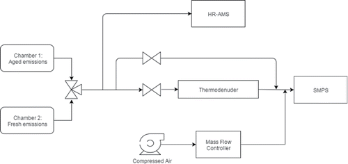
Figure 1 depicts the experimental setup for the experiments conducted during the FLAME-IV campaign relevant to this study. We used two smog chambers (7 m³ Teflon bags). In one (unperturbed) chamber, we studied fresh aerosol from emissions of the combusted fuel, whereas in the other (perturbed) chamber, we studied the properties of the aerosol after chemical aging (either photo-oxidation or dark ozonolysis). We alternated sampling from these two chambers on a 30-min duty cycle using an automated three-way valve. Instrumentation for experiments analyzing the chambers were housed in the Carnegie Mellon University (CMU) mobile air quality unit. We analyzed the primary emissions using this suite of instrumentation immediately after injection into the unperturbed chamber. We analyzed aged emissions by sampling from the perturbed chamber. Depending on the experiment, we either used ozone or UV photolysis to accomplish the aging. In two of the experiments, we injected nitrous acid in addition to exposure of the emissions to UV lights. The UV light photolyzes nitrous acid to increase hydroxyl radical concentrations and therefore increase overall oxidant exposure.

Figure 1. Experimental setup for gas-particle partitioning experiments during the FLAME-IV campaign.

3.2. Measurement of equilibration profiles

To thermally perturb the aerosol suspension, we operated a thermodenuder (91.4 cm length and 4.11 cm inner diameter) upstream of a scanning mobility particle sizer (SMPS, TSI, Shoreview, MN, USA), based on the design used in Saleh et al. (2008). The SMPS measured the aerosol size distributions for particles in the size range 12.2 ⩽ d_p ⩽ 736.5 nm. For all of the experiments conducted relevant to this study, we maintained the wall temperature of the thermodenuder at 50°C. The SMPS sampling alternated between this heated thermodenuder and an ambient temperature bypass tube. We drew a standard flow rate of 1 SLPM from the chambers through the thermodenuder, leading to a residence time in the thermodenuder of approximately 60 s. However, we varied this residence time by modulating the extraction flow rate using a mass flow controller (Figure 1). For the bulk of the experiments, we used residence times of 60, 160, 250, and 290 s. We estimated the particle mass concentrations from both the bypass and the thermodenuder by integrating the size distributions obtained from the SMPS assuming that the particles were spherical with a density of 1 g/cm³. For this analysis, the exact density has a minor contribution, but if the density (or particle shape) changed substantially upon heating this would introduce some error. However, these systems are OA dominated—observed BC to OA ratios are in the range of 0.01 to 0.05 (Tkacik et al. 2017) and therefore the OA is expected to form thick coatings over the BC cores leading to near spherical particles. BC is usually formed initially during a combustion event from biomass burning and subsequent organic vapors prefer to condense on the existing surface area of BC as opposed to form new (externally mixed) particles by nucleation.

To investigate equilibration time scales, we measured the change in the aerosol particle concentration (ΔC) at the different residence times in the thermodenuder. We assumed that equilibrium was achieved when ΔC reached a constant value with further increases in residence time. A linear interpolation between bypass scans taken before and after the residence time experiments for each condition and fuel combination (Table 1) was used to account for wall losses in the chamber. As shown in the methods of Saleh et al. (2011) and Saleh et al. (2012) and the theory above, we can use the dimensionless time, t* to retrieve the equilibration profile of a multi-component aerosol:[6] [7] [8]

Here ΔC_OA (equilibrium) is taken as ΔC_maximum which is the maximum change in the aerosol concentration from the experiments. C^v_i is the gas-phase (vapor) concentration of component i. Since we do not have gas-phase measurements of the semi-volatile compounds from the campaign, we applied a mass balance to build the equilibration profile. The change in the gas-phase concentration is equal to the change in particle mass concentration, which is much easier to measure. ΔC_OA represents the change in particle phase mass concentration; T_in and T_f are the initial and final temperatures. The process of optimally estimating the parameter α involves adjusting the dimensionless time, t*, as changing α changes the condensation sink and thus t/τ; thus the fitting procedure optimizes across the t/τ space until a best match, obtained by minimizing the sum of squares error, to the assumed non-dimensional function is obtained.

3.3. Determination of SOA fraction

For some of the experiments in which the emissions were aged, we used a high resolution time-of-flight aerosol mass spectrometer (HR-ToF-AMS) to measure sub-micron aerosol composition. Table 1 exhibits the estimated SOA fractions calculated in these experiments from the HR-ToF-AMS. We did not use this estimate in any of the quantitative analyses; it simply served as an indicator for the extent of chemical processing of the emissions. In order to distinguish between the fresh and aged aerosols, we adopted the residual analysis method of Sage et al. (2007) as extended by Grieshop et al. (2009) for biomass-burning emissions. This method relies on a single mass spectrum peak as a tracer for the primary biomass-burning organic aerosol. The total organic aerosol mass can be split into two components assuming that the mass spectrum of primary organic aerosol (POA) is constant throughout the experiment: MS_residual = MS_t − f_ion MS_POA. Here f_ion is the maximum fraction of primary mass (MS_POA) that contributes to the total OA mass (MS_t) and it is given by: .

4. Results and discussion

4.1. Effective accommodation coefficients of fresh and aged emissions

The data from the thermodenuder measurements used in this study were just one of the many areas of focus in the FLAME-IV campaign. Consequently, we could only obtain measurements at a few different residence times during any given experiment. To completely characterize an equilibration profile, it is important to have at least two data points at sufficiently long residence times to ensure that the particle diameters (and ΔC_OA) have reached an asymptotic value. We did not have sufficient data from any single burn to precisely characterize this equilibration, and especially for the fresh emissions we did not have sufficient data at longer residence times. To address this, we compiled measurements from multiple experiments (with a variety of fuels and burn conditions). We compiled the overall combined data and also separated the fresh and aged emissions data. We binned the data points in intervals of t/τ in order to preserve a roughly equal number of data points in each bin; for the combined and aged emissions we had sufficient data for five time bins, including two at relatively long residence times, while for the fresh emissions we had sufficient data for four bins. The binned data show considerable spread, which may be due to both measurement uncertainty as well as differences in mass-transfer limitations (i.e., α) of the OA from different burns. However, the medians of each of the bins reasonably follow the expected equilibration profile, and we use these values to obtain best-fit values for α.

Figure 2 shows the equilibration profiles we obtained from fitting the biomass-burning experiments and their agreement with the first-order dynamic response. In this analysis, the non-dimensional time (t* = t/τ) is a function of α because τ depends on α, so the exponential form of the first-order function shown as a black curve is fixed, and the data move in x as the value of α varies.

Figure 2. Equilibration profiles for (a) all emissions data, (b) fresh emissions data, and (c) aged emissions data from all experiments after applying the optimization routine. The accommodation coefficients (α) obtained for each case are shown on the respective graphs. Upon binning the scattered data, we see that it follows the behavior of the general dynamic response (GDR) curve.

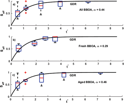
Figure 2a shows the combined data set from the entire experimental matrix, while Figure 2b shows the fresh emissions and Figure 2c shows the emissions which were aged in the chamber. The experimental observations we used to obtain these plots (listed in Table 1) were all obtained at relatively high C_OA loadings in the thermodenuder (35 μg m⁻³ ⩽ C_OA ⩽ 150 μg m⁻³) that are representative of plume conditions. Since the change in particle mass concentration (ΔC) was less than 30% in all the experiments and thus the condensation sink remained nearly constant, we could adopt a first-order dynamic response (Equation (2[2] )) to represent the equilibration profile of the aerosol systems (Saleh et al. 2012). Saleh et al. (2013) showed that secondary organic aerosol from α-pinene fall on the first-order response curve when plotted on dimensionless axes of S_eff and t* = t/τ, and in Figure 2 we see that the data from this study display a similar behavior.

The medians of the combined data reasonably follow an exponential approach to an asymptotic value. For both the combined and aged data, observations extend to t* = t/τ > 5 and are likely to have achieved equilibrium (Saleh et al. 2011); however, for the fresh primary emissions we had data only up to t* = t/τ ≃ 3.5. Regardless, even in this case the data appear to reasonably constrain the particle equilibration.

We obtained optimal values for α by fitting the equilibration profile (Equation (3[3] )) to the response curve (Equation (5[5] )) using the MATLAB function lsqnonlin (Mathworks Inc. 2015b). We obtain these values by optimizing the position of the data points by adjusting the value of α and therefore τ, to fit the response curve (Saleh et al. 2013). For the combined data shown in Figure 2a, we obtained α = 0.44; this corresponds well with the range of 0.28 to 0.46 for ambient organic aerosol estimated by Saleh et al. (2012). We also determined separate accommodation coefficients for fresh (Figure 2b, α = 0.29) and aged (Figure 2c, α = 0.46) biomass-burning aerosols. Given the experimental limitations mentioned above, we believe it is likely that the difference between the fresh and aged α is due to experimental variability. However, we can state with confidence that both have an α between 0.1 and 1, as shown by the following analysis.

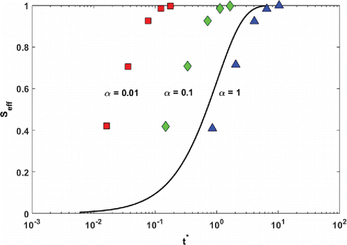
To demonstrate the effect of varying α on the fitting, in Figure 3 we show the combined median data for three different values: α = {0.01, 0.1, 1}. Because the accommodation coefficient—the fit parameter in this case—enters into the non-dimensional time, the effect is to move the data with respect to a fixed theoretical first-order equilibration function (shown as a black curve). When plotted on a semi-logarithmic x-axis, there is significant deviation from the universal response curve in the positioning of the data points when τ is calculated using this range of α values. The accommodation coefficient obtained from our investigation are fairly well constrained by the median data; they are bounded by 0.1 < α < 1, and our combined data estimate for α of 0.44, is closer to 1 than 0.1 on a logarithmic scale. The relatively large values of α obtained in this study for fresh and aged biomass-burning OA indicate that the severe diffusion limitations hypothesized to be associated with a glassy matrix are not evident in our results. However, since α < 1, there may still exist some barrier to mass transfer, which could be either in the condensed phase or at the particle–vapor interface. This is in contrast with the study of Vaden et al. (2011) who observed fast and slow evaporation rates in their experiments where vapors were continuously stripped from the gas phase and came to the conclusion of kinetic limitations. It is important to note that the experiments performed by Vaden et al. (2011) did not directly observe equilibration time scales, but rather evaporation rate, which depends on both kinetic and thermodynamic properties (volatility). The assumed volatility distribution in that study did not account for the extremely low volatility organic compounds (ELVOCs), which have been shown recently to constitute a fraction of SOA (Jokinen et al. 2015). Therefore, the kinetic limitations (α ≪ 1) invoked in Vaden et al. (2011) to interpret the measurements are likely an artifact of missing the ELVOCs portion of the volatility distribution. Even if ELVOCs exhibited condensed phase kinetic limitation, it would have a small effect on the equilibration profile because having a very low volatility (i.e., small saturation concentration, C_sat), they contribute a very small fraction of the total change in aerosol concentration in the thermodenuder. Therefore, from an equilibration point of view, the higher volatility components dictate the equilibration profile and consequently the effective α. If this were indeed the case, the α derived in this study can be considered representative of the higher volatility components that lead to large changes in mass when building the equilibration profile. The contribution of ELVOCs to the equilibration curve in this case is thus small to negligible and therefore the effective α that we get does not constrain these ELVOCs. However, it should be noted that in order to predict the evolution of OA in the atmosphere, constraining the α of ELVOCs plays a less important role, since they do not evaporate readily.

Figure 3. The binned data from the entire experimental matrix plotted with t* calculated from different values of α. This figure shows the significant deviation from the universal dynamic response with equilibration time scales calculated from logarithmically spaced accommodation coefficient values.

All of the accommodation coefficients presented above were based on an assumed average molecular mass, M = 200 g/mol, and gas-phase molecular diffusion coefficient, D = 5 × 10^{− 6} m²/s. We explored the sensitivity of α to these parameters by altering them together by 50%, assuming an inverse relationship between the two in Table 2. This range of M and D is representative of C₃ to C₁₀ dicarboxylic acids. From this analysis, we see that as the assumed molecular mass increases (and diffusion coefficient decreases) the fitted mass accommodation coefficient also increases. Since higher molecular mass is more likely for the extremely low volatility compounds associated with organic aerosols, this reinforces our conclusion that the mass accommodation coefficient for these particles is very close to (if not equal to) unity.

Table 2. Mass accommodation values found in this study for biomass burning emissions for different assumptions on molar mass and gas phase diffusion coefficient.

	Mass accommodation coefficient
Dataset		D =
Compiled data	0.44	0.3	0.72
Aged OA	0.46	0.29	0.89
Fresh OA	0.29	0.18	0.51

4.2. Atmospheric implications in a biomass-burning plume

In order to assess the atmospheric implications of the identified mass accommodation coefficient, we consider the behavior of a biomass-burning plume that gets progressively diluted in the atmosphere. The relatively rapid change in boundary conditions associated with plume dilution represents a stringent test to assess the deviation between OA loading calculated using the instantaneous equilibration assumption and detailed phase change dynamics.

We assume a lognormal particle size distribution typical of such a plume (median diameter of 175 nm and geometric standard deviation of 1.86), with an initial mass concentration (C_OA) of about 100 μg/m³, corresponding to typical wild-fire observations (Hobbs et al. 2003). To simulate equilibrium and dynamic partitioning in response to the dilution, we use the volatility distributions derived by May et al. (2013) from the biomass-burning smoke of common North American shrubs and grasses. This distribution describes primary emissions using a Volatility Basis Set (Donahue et al. 2006) with log ₁₀C° = { − 2, −1, 0, 1, 2, 3, 4} and f_i = {0.2, 0, 0.1, 0.1, 0.2, 0.1, 0.3} for an α of 1, f_i = {0.1, 0.1, 0, 0.2, 0.2, 0.1, 0.3} for an α of 0.1 and f_i = {0.2, 0, 0, 0.2, 0.2, 0.1, 0.3} for an α of 0.01. For the conditions of this simulation this means that roughly two-thirds of the emissions are “semi volatile” and one-third is “nonvolatile,” so the simulation provides a stringent test of the potential for dynamical effects to influence the organic aerosol concentration in the plume. We treat the dilution itself by assuming that the species from the plume are contained in a well-mixed volume that expands with time by entrainment of clean background air. The initial plume width y(0), therefore increases to y(t) at time t, which affects the concentrations in the box by dilution with the ambient air. We used the parameterization described by Trentmann et al. (2005) to estimate the plume width and dilution ratio at each time step. This parameterization uses a passive tracer, (carbon monoxide in this case) to estimate downwind concentrations of the smoke from the plume.

We calculate the mass-transfer dynamics using the partitioning equations for organic species i in particle population p:[9] [10] Here D is the diffusion coefficient, C°_i is the saturation concentration, F is the Fuchs–Sutugin transition-regime correction, K is the Kelvin term, m_{i, p} is the mass of species i in particle population p, X_{i, p} is the mass fraction of species i in that population, and C_OA is the total particle-phase organic aerosol concentration. By using the mass fraction to calculate the saturation mass concentration, we are employing a “pseudo-ideal” approximation in which the particle-phase activity is given by the mass and not the mole fraction; however, we also assume a single value for the gas-phase diffusion coefficient and mass accommodation coefficient, and so effectively assume a single value for the organic molecular weight. The equilibrium organic aerosol concentration is given by[11] where C^tot_i is the total (vapor and condensed-phase) mass concentration of species i and ξ_i is the partitioning coefficient for compound i.

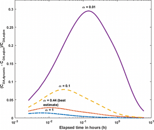
We calculate the ratio of dynamic to equilibrium organic-aerosol concentrations in a plume simulation using four different values of the mass accommodation coefficient: α = (0.01, 0.1, 1) and our best-estimate value α = 0.44. In Figure 4, we show the relative difference in OA concentration between the dynamic and equilibrium values as a function time as the model plume undergoes isothermal dilution. Because dilution drives evaporation, the dynamic values always exceed the equilibrium values, and lower values of α enhance this difference by delaying evaporation. If α were to be 0.01, there would be a maximum error of 30% approximately 10 min downwind of the source if a model assumed instantaneous equilibrium; however, for our best estimate of α = 0.44, the error is a maximum of around 3%. After an hour of dilution in the atmosphere (at which point C_OA < 10 μg/m³), the dynamic scenario for all accommodation coefficients start to approach the equilibrium case. These results indicate that the assumption of instantaneous equilibrium adopted in atmospheric models can adequately be used to represent the evolution of biomass-burning OA loading in the atmosphere.

Figure 4. Fractional difference between dynamic and equilibrium cases simulating dispersion of a biomass-burning plume for a range of values of the mass accommodation coefficient α. After about an hour the dynamic and equilibrium cases converge and the relative difference is small regardless of the assumed value of α, but for the best-estimate value (α = 0.44) at no time does the error in the equilibrium partitioning calculation exceed 7%.

5. Conclusions

We applied the methods of Saleh et al. (2012, 2013) to determine effective mass accommodation coefficients of complex aerosol systems from experiments carried out in the FLAME-IV campaign. We studied biomass burning organic aerosol generated from these experiments, from different fuel types for both, fresh and aged conditions. We characterized equilibration profiles as well as effective mass accommodation coefficients for fresh (Figure 2b) and aged aerosol (Figure 2c). We observed that for both fresh and aged aerosol, α is constrained between 0.1 and 1.0, indicating that diffusion limitations associated with a glassy matrix were not present. If these limitations were present, it would be apparent in an α lower by an order of magnitude than the values obtained here. This derived α may however pertain only to the higher volatility components of BBOA which contributed most to the observed equilibration profile and possibly does not constrain lower volatility components in the ELVOC range.

Finally, we used a plume dilution model to assess the magnitude of the error associated with the instantaneous equilibrium assumption as opposed to a full dynamic model over a range of magnitudes of α including the α obtained in this study for BBOA. We found that for α > 0.1, the error between the instantaneous and dynamic models never exceeds 7% giving credence to the continued application of this assumption in atmospheric models.

Additional information

Funding

This research was supported by grants ER65296 from the Department of Energy Atmospheric System Research Program and CHE1412309 from the National Science Foundation.

References

- Bond, T. C., Streets, D. G., Yarber, K. F., Nelson, S. M., Woo, J. H., and Klimont, Z. (2004). A Technology-Based Global Inventory of Black and Organic Carbon Emissions from Combustion. J. Geophys. Res. Atmos., 109(14):1–43.
- Christian, T. J. (2004). Comprehensive Laboratory Measurements of Biomass-Burning Emissions: 2. First Intercomparison of Open-Path FTIR, PTR-MS, and GC-MS/FID/ECD. J. Geophys. Res., 109(D2):1–12.
- Davis, E. (2006). A History and State-of-the-Art of Accommodation Coefficients. Atmos. Res., 82(3):561–578.
- Donahue, N. M., Robinson, A. L., Stanier, C. O., and Pandis, S. N. (2006). Coupled Partitioning, Dilution, and Chemical Aging of Semivolatile Organics. Environ. Sci. Technol., 40(8):2635–2643.
- Grieshop, A. P., Donahue, N. M., and Robinson, A. L. (2009). Laboratory Investigation of Photochemical Oxidation of Organic Aerosol from Wood Fires 2: Analysis of Aerosol Mass Spectrometer Data. Atmos. Chem. Phys., 9(6):2227–2240.
- Hennigan, C. J., Miracolo, M. A., Engelhart, G. J., May, A. A., Presto, A. A., Lee, T., Sullivan, A. P., McMeeking, G. R., Coe, H., Wold, C. E., Hao, W. M., Gilman, J. B., Kuster, W. C., De Gouw, J., Schichtel, B. A., Collett, J. L., Kreidenweis, S. M., and Robinson, A. L. (2011). Chemical and Physical Transformations of Organic Aerosol from the Photo-Oxidation of Open Biomass Burning Emissions in an Environmental Chamber. Atmos. Chem. Phys., 11(15):7669–7686.
- Hobbs, P. V., Sinha, P., Yokelson, R. J., Christian, T. J., Blake, D. R., Gao, S., Kirchstetter, T. W., Novakov, T., and Pilewskie, P. (2003). Evolution of Gases and Particles from a Savanna Fire in South Africa. J. Geophys. Res. Atmos., 108(D13).
- Jimenez, J. L., Canagaratna, M. R., Donahue, N. M., Prevot, A. S. H., Zhang, Q., Kroll, J. H., DeCarlo, P. F., Allan, J. D., Coe, H., Ng, N. L., Aiken, A. C., Docherty, K. S., Ulbrich, I. M., Grieshop, A. P., Robinson, A. L., Duplissy, J., Smith, J. D., Wilson, K. R., Lanz, V. A., Hueglin, C., Sun, Y. L., Tian, J., Laaksonen, A., Raatikainen, T., Rautiainen, J., Vaattovaara, P., Ehn, M., Kulmala, M., Tomlinson, J. M., Collins, D. R., Cubison, M. J., Dunlea, J., Huffman, J. A., Onasch, T. B., Alfarra, M. R., Williams, P. I., Bower, K., Kondo, Y., Schneider, J., Drewnick, F., Borrmann, S., Weimer, S., Demerjian, K., Salcedo, D., Cottrell, L., Griffin, R., Takami, A., Miyoshi, T., Hatakeyama, S., Shimono, A., Sun, J. Y., Zhang, Y. M., Dzepina, K., Kimmel, J. R., Sueper, D., Jayne, J. T., Herndon, S. C., Trimborn, A. M., Williams, L. R., Wood, E. C., Middlebrook, A. M., Kolb, C. E., Baltensperger, U., and Worsnop, D. R. (2009). Evolution of Organic Aerosols in the Atmosphere. Science, 326(5959):1525–1529.
- Jokinen, T., Berndt, T., Makkonen, R., Kerminen, V.-M., Junninen, H., Paasonen, P., Stratmann, F., Herrmann, H., Guenther, A. B., Worsnop, D. R., Kulmala, M., Ehn, M., and Sipila, M. (2015). Production of Extremely Low Volatile Organic Compounds from Biogenic Emissions: Measured Yields and Atmospheric Implications. Proc. Natl. Acad. Sci., 112(23):7123–7128.
- Julin, J., Winkler, P. M., Donahue, N. M., Wagner, P. E., and Riipinen, I. (2014). Near-Unity Mass Accommodation Coefficient of Organic Molecules of Varying Structure. Environ. Sci. Technol., 48(20):12083–12089.
- Koop, T., Bookhold, J., Shiraiwa, M., and Pöschl, U. (2011). Glass Transition and Phase State of Organic Compounds: Dependency on Molecular Properties and Implications for Secondary Organic Aerosols in the Atmosphere. Phy. Chem. Chem. Phys., 13(43):19238–19255.
- Lehtinen, K. E., Korhonen, H., Maso, M., and Kulmala, M. (2003). On the Concept of Condensation Sink Diameter. Bore. Environ. Res., 8(4):405–412.
- Liu, P., Li, Y. J., Wang, Y., Gilles, M. K., Zaveri, R. A., Bertram, A. K., and Martin, S. T. (2016). Lability of Secondary Organic Particulate Matter. Proc. Natl. Acad. Sci, 113(45):12643–12648.
- May, A. A., Levin, E. J. T., Hennigan, C. J., Riipinen, I., Lee, T., Collett, J. L., Jimenez, J. L., Kreidenweis, S. M., and Robinson, A. L. (2013). Gas-Particle Partitioning of Primary Organic Aerosol Emissions: 3. Biomass Burning. J. Geophys. Res. Atmos., 118(19):11327–11338.
- McMeeking, G. R., Kreidenweis, S. M., Baker, S., Carrico, C. M., Chow, J. C., Collett, J. L., Hao, W. M., Holden, A. S., Kirchstetter, T. W., Malm, W. C., Moosmller, H., Sullivan, A. P., and Cyle E. W. (2009). Emissions of Trace Gases and Aerosols During the Open Combustion of Biomass in the Laboratory. J. Geophys. Res. Atmos., 114(19):1–20.
- Nel, A. (2005). Air Pollution – Related Illness : Effects of Particles. Science, 308(5723):804–806.
- O’Neill, N. T., Eck, T. F., Holben, B. N., Smirnov, A., Royer, A., and Li, Z. (2002). Optical Properties of Boreal Forest Fire Smoke Derived from Sun Photometry. J. Geophys. Res., 107(D11):AAC 6–1–AAC 6–19.
- Pankow, J. F. (1994). An Absorption Model of Gas/Particle Partitioning of Organic Compounds in the Atmosphere. Atmos. Environ., 28:185–188.
- Pope III, C. A., and Dockery, D. W. (2006). Health Effects of Fine Particulate Air Pollution: Lines that Connect. J. Air Waste Manag. Assoc. (1995), 56(November):709–742.
- Renbaum-Wolff, L., Grayson, J. W., Bateman, A. P., Kuwata, M., Sellier, M., Murray, B. J., Shilling, J. E., Martin, S. T., and Bertram, A. K. (2013). Viscosity of α-Pinene Secondary Organic Material and Implications for Particle Growth and Reactivity. Proc. Natl. Acad. Sci., 110(20):8014–8019.
- Robinson, A. L., Donahue, N. M., Shrivastava, M. K., Weitkamp, E. A., Sage, A. M., Grieshop, A. P., Lane, T. E., Pierce, J. R., and Pandis, S. N. (2007). Rethinking Organic Aerosols: Semivolatile Emissions and Photochemical Aging. Science (New York, N.Y.), 315:1259–1262.
- Sage, A. M., Weitkamp, E. A., Robinson, A. L., and Donahue, N. M. (2007). Evolving Mass Spectra of the Oxidized Component of Organic Aerosol: Results from Aerosol Mass Spectrometer Analyses of Aged Diesel Emissions. Atmos. Chem. Phys. Discuss., 7(4):10065–10096.
- Saleh, R., Donahue, N. M., and Robinson, A. L. (2013). Time Scales for Gas-Particle Partitioning Equilibration of Secondary Organic Aerosol Formed From Alpha-Pinene Ozonolysis. Environ. Sci. Technol., 47(11):5588–5594.
- Saleh, R., Khlystov, A., and Shihadeh, A. (2012). Determination of Evaporation Coefficients of Ambient and Laboratory-Generated Semivolatile Organic Aerosols from Phase Equilibration Kinetics in a Thermodenuder. Aerosol Sci. Technol., 46(1):22–30.
- Saleh, R., Shihadeh, A., and Khlystov, A. (2011). On Transport Phenomena and Equilibration Time Scales in Thermodenuders. Atmos. Meas. Tech., 4(3):571–581.
- Saleh, R., Walker, J., and Khlystov, A. (2008). Determination of Saturation Pressure and Enthalpy of Vaporization of Semi-Volatile Aerosols: The Integrated Volume Method. J. Aerosol Sci., 39(10):876–887.
- Seinfeld, J. H., and Pandis, S. N. (2016). Atmospheric Chemistry and Physics: From Air Pollution to Climate Change. John Wiley & Sons, New York.
- Shiraiwa, M., Ammann, M., Koop, T., and Poeschl, U. (2011). Gas Uptake and Chemical Aging of Semisolid Organic Aerosol Particles. Proc. Natl. Acad. Sci., 108(27):11003–11008.
- Solomon, S. (2007). Climate Change 2007–the Physical Science Basis: Working Group I Contribution to the Fourth Assessment Report of the IPCC. Vol. 4. Cambridge University Press, Cambridge.
- Stockwell, C., Yokelson, R., Kreidenweis, S., Robinson, A., DeMott, P., Sullivan, R., Reardon, J., Ryan, K., Griffith, D. W., and Stevens, L. (2014). Trace Gas Emissions from Combustion of Peat, Crop Residue, Domestic Biofuels, Grasses, and Other Fuels: Configuration and Fourier Transform Infrared (FTIR) Component of the Fourth Fire Lab at Missoula Experiment (Flame-4). Proc. Natl. Acad. Sci., 14(18):9727–9754.
- Tkacik, D. S., Robinson, E. S., Ahern, A., Saleh, R., Stockwell, C., Veres, P., Simpson, I. J., Meinardi, S., Blake, D. R., Yokelson, R. J., Presto, A. A., Sullivan, R. C., Donahue, N. M., and Robinson, A. L. (2017). A Dual-Chamber Method for Quantifying the Effects of Atmospheric Perturbations on Secondary Organic Aerosol Formation from Biomass Burning Emissions. J. Geophys. Res. Atmos., 122(11):6043–6058.
- Trentmann, J., Yokelson, R. J., Hobbs, P. V., Winterrath, T., Christian, T. J., Andreae, M. O., and Mason, S. A. (2005). An Analysis of the Chemical Processes in the Smoke Plume from a Savanna Fire. J. Geophys. Res. Atmos., 110(D12).
- Vaden, T. D., Imre, D., Beránek, J., Shrivastava, M., and Zelenyuk, A. (2011). (suppl.)Evaporation Kinetics and Phase of Laboratory and Ambient Secondary Organic Aerosol. Proc. Natl. Acad. Sci. USA, 108(6):2190–2195.
- Vehkamäki, H., and Riipinen, I. (2012). Thermodynamics and Kinetics of Atmospheric Aerosol Particle Formation and Growth. Chem. Soc. Rev., 41:5160–5173.
- Wexler, A. S., and Seinfeld, J. H. (1990). The Distribution of Ammonium-Salts Among a Size and Composition Dispersed Aerosol. Atmos. Environ., 24(5):1231–1246.
- Wiedinmyer, C., Akagi, S. K., Yokelson, R. J., Emmons, L. K., Al-Saadi, J. A., Orlando, J. J., and Soja, A. J. (2010). The Fire INventory from NCAR (FINN) – A High Resolution Global Model to Estimate the Emissions from Open Burning. Geosci. Model Develop. Discuss., 3(4):2439–2476.
- Yatavelli, R. L. N., Stark, H., Thompson, S. L., Kimmel, J. R., Cubison, M. J., Day, D. A., Campuzano-Jost, P., Palm, B. B., Hodzic, A., Thornton, J. A., Jayne, J. T., Worsnop, D. R., and Jimenez, J. L. (2014). Semicontinuous Measurements of Gas-Particle Partitioning of Organic Acids in a Ponderosa Pine Forest using a MOVI-HRToF-CIMS. Atmosph. Chem. Phys., 14(3):1527–1546.
- Ye, Q., Robinson, E. S., Ding, X., Ye, P., Sullivan, R. C., and Donahue, N. M. (2016). Mixing of Secondary Organic Aerosols Versus Relative Humidity. Proc. Natl. Acad. Sci., 113(45):12649–12654.
- Yokelson, R. J., Crounse, J. D., DeCarlo, P. F., Karl, T., Urbanski, S., Atlas, E., Campos, T., Shinozuka, Y., Kapustin, V., Clarke, A. D., Weinheimer, A., Knapp, D. J., Montzka, D. D., Holloway, J., Weibring, P., Flocke, F., Zheng, W., Toohey, D., Wennberg, P. O., Wiedinmyer, C., Mauldin, L., Fried, A., Richter, D., Walega, J., Jimenez, J. L., Adachi, K., Buseck, P. R., Hall, S. R., and Shetter, R. (2009). Emissions from Biomass Burning in the Yucatan. Atmos. Chem. Phys., 9:5785–5812.