Determination of the aerosol particle size distribution by means of the diffusion battery: Analytical inversion

Abstract

The algorithm of the analytical inversion of aerosol size distribution is proposed in this work. As the diffusion battery separates particles into several fractions according to their diffusivity, the total spectrum can be represented as the sum of spectra of fractions. Analytical formulas are derived to calculate mean diameters for particles in different fractions using diffusion battery penetrations as input parameters. The spectra of fractions are approximated by lognormal functions. Two analytical solutions for the aerosol size distribution inversion problem are discussed. The sizing accuracy of analytical solutions is investigated, comparing them with the measurements through transmission electron microscopy using the laboratory-generated NaCl aerosol. The agreement is demonstrated to be within 10% accuracy. It is shown that in case of two-mode size distribution, the spectrum components are well resolved for rather distant peaks (modal diameters of 10 and 300 nm) and poorly resolved for nearby modes (50 and 300 nm). To improve the peak resolution, the procedure of spectrum correction is applied demonstrating an excellent peak separation. Finally, the peak resolution is experimentally verified for the laboratory-generated two-mode spectra of tungsten oxide–NaCl aerosol with the modal diameters of 10 and 60 nm, respectively. Both analytical solutions demonstrated good peak resolution.

Copyright © 2018 American Association for Aerosol Research

EDITOR:

• Jingkun Jiang

1. Introduction

During the past few decades, the need to measure aerosol properties has increased tremendously , therefore, refined techniques are necessary to control the dynamics of aerosol pollution from industrial activity, volcanic eruptions, cigarette smoke, motor vehicle emissions, and resuspended soil (Harrison 1986; Chow 1995; Colbeck 1995; Giechaskiel et al. 2014; Amaral et al. 2015). On the contrary, new technologies for “desirable” aerosol production are developed by material scientists and engineers to produce nanopowders and pigments (Guo et al. 2010; Gevorkyan et al. 2017), nanoaerosol drugs (Onischuk et al. 2014, 2016), and flowing precursors for chemical reactors (Powell et al. 2017). Aerosol measurements are of immense importance in these applications.

Aerosol concentration and size distribution are valuable data, when studying the aerosol properties. Nanosized particles are difficult to measure optically due to weak light scattering. Impaction techniques can be used to characterize these particles only at pressures much lower than atmospheric. One of the widely used approaches for sizing ultrafine particles is electrical mobility techniques, which are based on the measurement of charged particle migration in the electric field. The critical point in electrical mobility methods is in the production of a known particle charge distribution. A number of physical charging processes are used, including charging by small gas ions, photoemission, thermionic emission, and others. However, none of these charging techniques result in a reproducible charge distribution, creating problems in quantitative measurements of particle size distribution (Flagan 2011). An alternative to electrical mobility methods is the diffusion battery (DB), which is used to separate particles by diffusion mobilities (Knutson 1999). The diffusion battery technique is simple and does not need particle charging. Screen-type diffusion batteries became popular among scientists after the publication of a series of papers (Cheng and Yeh 1980; Cheng et al. 1980, 1985), which showed that the fan-model filtration theory can be used to describe the particle capture by wire screens. Screen-type diffusion battery is simple and compact. It is organized as a consequence of compartments (sections) filled by stacks of screens. As the aerosol passes through the battery, the particles are captured by screens. Aerosol penetrations through different numbers of sections are linked with the particle size spectrum. However, to retrieve the particle size distribution from aerosol penetrations through screen stacks, one should solve an inverse problem, which is mathematically complex and ambiguous, as many different spectra can result from the same set of penetrations. Graphical, analytical, and numerical approaches were elaborated to determine the aerosol size spectrum from DB measurements (see the references and the discussion in more detail in Onischuk et al. (2018)). However, the graphical/analytical methods are either too much laborious or limited by a single-mode size distribution. The problem of the numerical methods is in the non-uniqueness of the solution and mathematically complex algorithm. Therefore, a simple and non-ambiguous methods giving a one-to-one correspondence between the particle size distribution and DB measurements are still of need.

In our previous work (Onischuk et al. 2018), we proposed a new method to determine the aerosol size distribution from the diffusion battery penetrations. The central idea of this method was to obtain the particle diameter frequency distribution using simple analytical formulas (analytical inversion). The total size distribution was considered as a sum of the spectra of fractions, that is, spectra of particles captured by different diffusion battery sections. The input parameters for these formulas were aerosol concentrations measured down-flow of each section. Different analytical formulas can be derived linking the diffusion battery penetrations with the spectra of fractions. In our previous paper we considered one of the possible analytical approaches. In the present work we represent analytical formulas for this approach in a more concise form. We also derive new analytical formulas using another analytical approach. Besides, we elaborated the mathematical procedure improving the size spectrum resolution for analytical inversion. Both sizing accuracy and resolution of analytical solutions are demonstrated in the laboratory measurements of single- and two-mode aerosol.

2. Analytical inversion

In this work (as well as in our previous one [Onischuk et al. 2018]), we use the diffusion battery comprising nine consecutive sections, which are filled with the stacks of woven nylon screens. The number of screens is 2, 2, 4, 8, 16, 32, 64, 128, and 256 for the section numbers 1, 2, …, 9, respectively. The aerosol passes through the battery starting from section 1. The aerosol concentrations are measured by a Condensation Particle Counter (CPC) at the inlet of diffusion battery and downstream of each section using T-junctions (for more detail see (Onischuk et al. 2018)). The particle diameter distribution function f(D) can be calculated from the DB penetrations g_i: [1] where C_i and C₀ are particle number concentrations measured downstream of the i-th section and at the inlet of diffusion battery, respectively, i is the number of section. We consider the size distribution function normalized to unity. To deduce the function f(D) from DB penetrations, one must solve the Fredholm integral equations of the first kind (Phillips 1962): [2] where a and b are the limits of size interval, ε_i are the experimental errors, and K_i(D) is kernel function for the diffusion battery: [3] which is the probability for a particle of diameter D to penetrate through the sequence of diffusion battery sections with numbers from 1 to i; is the single-fiber collection efficiency for particles of diameter D, is the total number of screens in the sequence of sections from 1 to i, that is,  = n₁+n₂+…+n_i (where n₁, …, n_i are the numbers of screens in sections 1, …, i, respectively), , where α = 0.231 is the screen solid volume fraction, h = 1.13 × 10^–2 cm is the screen thickness, and r = 2.5 × 10⁻³ cm is the radius of fibers in the screen.

Usually, the particle size distribution is represented in the finite-dimensional form to solve Equation (2)[2] (Crump and Seinfeld 1982). But, the exact solution is practically always too much oscillatory and differs disastrously from the real spectrum. Moreover, larger the number of DB sections, the higher are the frequencies introduced, which worsens the discrepancies between the solution and the real spectrum (Twomey 1965). Therefore, to obtain a realistic spectrum, some mathematical constraints are to be imposed to cut-off the non-physical, highly fluctuating solutions. Different mathematical approaches were elaborated to solve the ill-posed inversion problem Equation (2)[2] (for more detail, see Knutson 1999 and Onischuk et al. 2018). The purpose of this article is to derive analytical inversion formulas, giving the frequency distribution of particle single-fiber collection efficiency. In this case, the constraint is in approximation with the spectra of fractions of particles collected by different DB sections using single-mode size distributions.

The function is U-shaped with the minimum at D = 1100 nm for DB parameters used in this article (Onischuk et al. 2018), that is, the range of diameters for our battery is D < 1100 nm where one-to-one correspondence exists between μ and the particle diameter. The contribution to μ from the particle inertial impaction is negligible in the range D < 1100 nm (see Onischuk et al. 2018), therefore only two mechanisms are to be considered for the particle collection by screens: diffusion and interception: [4] where μ_D and μ_R are the single-fiber collection efficiencies for diffusion and interception, respectively, μ_DR is the diffusion–interception interaction term. The diffusion term can be expressed as (Kirsch et al. 1969) [5] where [6] is the Peclet number, U₀ = 0.85 cm/s is the linear flow velocity through the DB sections, is the particle diffusion coefficient, k is the Boltzmann constant, T is absolute temperature, η is the gas dynamic viscosity equal to η = 1.84 × 10⁻⁴ poise for air at room temperature, and C_C is the Cunningham correction factor equal to (Fuchs 1964; Reist 1993): [7] where λ = 65 nm is the gas mean free pass for air, A, Q, and b are parameters equal to A = 1.252, Q = 0.399, b = 1.100 (Reist 1993). The interception term is [8] where is the hydrodynamic parameter, is the interception parameter. The interaction term follows the expression [9]

Equation (4)[4] is the basis of the classical filtration theory. To calculate the overall collection efficiency, the efficiencies due to individual mechanisms are included additively and the correction term is incorporated to compensate the combined effect (Kirsch et al. 1969). However, Equation (4)[4] cannot be justified in a rigorous theoretical way. To predict the aerosol filtration by fibrous filters more exactly, Yeh and Liu (1974) calculated the single-fiber collection efficiency numerically for the continuum and the slip-flow regimes, considering diffusion, interception, and inertial impaction simultaneously. The calculated overall collection efficiency was in good agreement with the formula Equation (4)[4] for the range of interception parameter R < 0.05. Hunt et al. (2014) calculated the single-fiber efficiency from the collision rate for particles with fibers. They applied the Langevin equation for particle motion, which enabled consideration of all filtration mechanisms simultaneously. The calculated filtration efficiencies were in good agreement with those determined from Equation (4)[4] for R < 0.03.

In this work, we consider the aerosol spectra to be in the range of diameters 3 ≤ D ≤ 1100 nm, which corresponds to the range for the interception parameter 3 × 10⁻⁶ < R < 0.02. Therefore, one should expect that Equation (4)[4] well describes the collection efficiency for our experimental conditions. Moreover, the experimentally measured collection efficiencies (Cheng et al. 1980, 1985) also well agree with those calculated from the additive formula Equation (4)[4] for R < 0.02. Therefore in the following considerations, we link the single-fiber collection efficiency with the particle diameter through Equations (4)–(9).

For m sections of diffusion battery in an ideal case of , Equation (2)[2] takes the form [10]

As discussed by Onischuk et al. (2018), the linear combination of Equation (10)[10] is: [11] where and the functions are as follows [12]

The quantities h₁, h₂, …, h_m−1 are the fractions of particles collected by sections 1, 2, …, m − 1, respectively, and h_m is the fraction of the rest of the particles at the outlet of the section m − 1. The functions are the size spectra of the corresponding fractions of particles. The size distribution for original particles at the inlet of diffusion battery is equal to the sum of the spectra of fractions. [13]

According to Onischuk et al. (2018), the functions are approximated by the lognormal distribution [14] where D_i is the mean diameter of particles of the i-th fraction and σ is the standard geometric deviation (SGD), which is set uniformly for all fractions. Thus, the original spectrum is approximated by [15]

One should note that the functions are normalized to unity in the present article as in contrast with our previous work (Onischuk et al. 2018), which makes the following derivations of analytical formulas more transparent. We suppose that the value of SGD for any mode in the real spectrum cannot be less than that for the self-preserving spectrum equal to about σ_∞ ≈ 1.35. Therefore, we set σ = 1.35 in Equation (14)[14] . This value of SGD is small enough to resolve any mode in the real spectrum (see for more detail Onischuk et al. 2018).

In the case of polydisperse particles with the size distribution function φ_i, to describe the probability to penetrate through a stack of N screens one should use the following formula instead of Equation (3)[3] [16] where C and C₀ are the outlet and inlet aerosol concentrations, respectively, is the apparent (mean) single-fiber collection efficiency. Using Equation (16)[16] , one can determine measuring the inlet and outlet concentrations. Then, using Equations (4)–(9), one can calculate the mean particle diameter from . However, is a function of N (Onischuk et al. 2018), therefore, the apparent (mean) diameter will be a function of N. Hence, one should choose correctly the number of screens in the stack to evaluate the mean diameter for polydisperse aerosol. Optimally, the number of screens should be chosen in such a way to give far from zero and considerably less then unity.

Now, our task is to derive analytical expressions linking the diffusion battery penetrations g_i with the mean single-fiber collection efficiencies for fractions of particles collected by DB sections. For this purpose, we introduce the quantity , which is the mean single-fiber collection efficiency in the k-th section filled with n_k screens for the aerosol passed through the previous k – 1 sections (or for the inlet aerosol in the case of k = 1): [17]

It will also be useful to introduce the quantity , which is the mean single-fiber collection efficiency in the series of sections l, …, l+s with the total number of screens N_l,l+s = n_l + n_l+1 + … + n_l+s for the particles which passed before through the first l–1 sections of the diffusion battery: [18]

In the subsequent parts of the article, we will consider two analytical approaches (analytical solutions) giving the mean single-fiber collection efficiencies for fractions of particles separated by the diffusion battery sections. One of these solutions was considered in our previous paper (Onischuk et al. 2018), and now we give more concise expressions for this approach.

3. Analytical solutions

3.1. Solution 1

First, we will find the mean diameter D₁ for the first-fraction particles, that is, for the particles collected by the first section of the diffusion battery. For this purpose, we consider the original size distribution function f(D) as a sum of two parts ξ₁(D) and φ₁(D): [19] where and are size distribution functions for particles penetrated through the first section (the first-group particles) and those collected by the first section of diffusion battery (the second-group particles), respectively. Thus, the second-group particles are actually the first DB fraction. The portions of the first- and second-group particles in the whole spectrum are g₁ and h₁, respectively, following the relationships [20] [21] [22]

On the contrary, the quantity g₁ (which is actually the mean probability for the incoming particles to penetrate through the first section) is governed by Equation (10)[10] [23]

Substituting Equation (19)[19] into (23) we get [24]

The first and second integrals in Equation (24)[24] are governed by mean probabilities for the first- and second-group particles, respectively, to penetrate through the first section of diffusion battery. Using Equations (16)[24] , (21)[21] , and (22)[22] , these integrals can be expressed as [25] [26] where is the mean single-fiber collection efficiency for the second-group particles in the first section of the diffusion battery filled by n₁ screens, and is the mean single-fiber collection efficiency in a stack of n₁ screens for the first-group particles. Substituting Equations (25)[25] and (26)[26] into (24), we obtain [27]

The screens in our diffusion battery are distributed in such a way that n₁ = n₂, therefore, [28]

Taking into account the fact that the penetration g₂ is (see Equation (17)[17] ) [29] where is the mean single-fiber collection efficiency in the second DB section for particles penetrated through the first section, we obtain the following from Equations (20)[20] , (27)–(29): [30]

Equation (30)[30] is a rigorous formula for the mean single-fiber collection efficiency . Substituting instead of μ in Equation (4)[4] and solving Equations (4)–(9) numerically, we obtain the mean diameter D₁ for the first-fraction particles, that is, those collected by the first section of the diffusion battery.

To calculate the collection efficiencies for other fractions (1 < i < m), that is, for the particles collected by sections 2, …, m − 1, we use the same approach as for the first fraction, but the final formula is more complex than Equation (30)[30] . The reason for formula complication is the numbers of screens in the neighboring sections i and i + 1 , which are linked using the formula n_i+1= 2n_i as in contrast to the numbers of screens for sections 1 and 2, which follow the relationship n₁= n₂. When deriving the formula for the collection efficiency _, we consider the penetration of a parcel of particles with size distribution through n_i+1 screens. The sought for quantity cannot be determined rigorosly from DB penetrations, but it can be expressed using (see the online supplementary information (SI) for more detail): [31]

The quantity cannot be determined directly as well; however, taking into account that n_i+1=2n_i and consequently and using Equations (18)[18] and (19)[19] , we can approximate by the following interpolation formula [32]

Substituting Equation (32)[32] into (31), we obtain [33]

The complete derivation of Equation (33)[33] is given in the online SI.

For i = m, we have a rigoros formula for the mean collection efficiency for the particles of the last fraction, that is, those penetrated through the section m–1 (see Equation (17)[17] ): [34]

Substituting and instead of μ in Equation (4)[4] and solving Equations (4)–(9) numerically, we obtain the mean diameter D_i for the i-th fraction particles. This mean diameter is equal to the diameter of monodisperse particles with the same penetration through a stack of (or n_m) screens. Then, using Equations (14)[14] and (15)[15] , we obtain the size spectrum of original particles.

To check the validity of interpolation formula (Equation (32)[32] ), we compare the mean single-fiber collection efficiencies calculated by Equation (32)[32] with those determined directly using formulas Equations (17)[17] and (18)[18] . For this purpose, we numerically calculated the penetrations for the model size distribution function (Figure 1a) [35] with D₁ = 50 nm, D₂ = 300 nm, and σ₁ = σ₂ = 1.4. The penetrations g₁, …, g₉ for this spectrum as calculated numerically using Equations (10)[10] and (3)–(9) are 0.914, 0.841, 0.724, 0.567, 0.399, 0.248, 0.118, 0.031, 0.0028, respectively. Figure 2 shows the mean single-fiber collection efficiencies for the spectrum Equation (35)[35] as determined directly by using Equations (17)[17] and (18)[18] (spheres) and that determined by Equation (32)[32] (squares). Dash lines are the spline interpolations for spheres. One can see a good agreement between these two calculation methods. The discrepancy between squares and spheres does not exceed 0.5%, that is, Equation (32)[32] allows calculation with the accuracy much better than the typical experimental error in the measurements of DB penetrations (5%).

Figure 1. Original model two-mode spectrum (Equation (35)[35] , modal diameters D₁ = 50 nm, D₂ = 300 nm, and σ₁ = σ₂ = 1.4) (a), and spectra recovered analytically as the sum of lognormal functions Equations (14)[14] and (15)[15] with D_i calculated numerically using Equations (30)[30] , (33)[33] , and (34)[34] (solution 1) (b), and Equations (30)[30] , (34)[34] , (38)[38] , and (40)[40] (solution 2) (c). The contributions from different fractions to the inversely calculated spectra are shown by vertical lines.

Figure 2. Mean single-fiber collection efficiencies for the spectrum Equation (35)[35] (see Figure 1a) as determined directly using the numerically calculated penetrations and formulas Equations (17)[17] and (18)[18] (spheres), using Equation (32)[32] (squares) and Equation (37)[37] (diamonds). Dash lines are spline interpolations of solid symbols.

3.2. Solution 2

We refer to Equations (30)[30] , (33)[33] , and (34)[34] as solution 1. An alternative algorithm to calculate the mean collection efficiencies for the fractions of particles is proposed by Onischuk et al. (2018). We refer to this alternative way as solution 2. The quantities and are obtained in the latter approach as in solution 1, that is, using Equations (30)[30] and (34)[34] . But, for other fractions of particles, that is, for 1 < i < m, the mean single-fiber collection efficiencies are determined using another algorithm, considering the penetration of a parcel of particles with the size distribution through a stack of = n_i + n_i+1 screens. As a result, the mean collection efficiency is expressed using (see the online SI for more detail): [36]

To determine the interpolation formula, Equation (32)[32] is used. In this case, we assume that: for aerosol coming out of the i-th section, the mean single-fiber efficiency of particle collection in a stack of n_i + n_i+1 screens can be considered as the arithmetic mean of the collection efficiencies in stacks with n_i+1 and (n_i+1 + n_i+2) screens: [37]

The values of calculated using Equation (37)[37] are compared with those determined directly using formulas Equations (17)[17] and (18)[18] (see diamonds in Figure 2). The agreement between Equation (37)[37] , and the rigoros formulas Equations (17)[17] and (18)[18] were found to be within 1% of accuracy, which is better than the experimental accuracy of DB measurements.

Taking into account n_i+1 = 2n_i ,we obtain the following from Equations (36)[36] and (37)[37] [38]

In the case of i = m – 1, Equation (37)[37] cannot be used as the penetration because g_i+2 does not exist for i = m – 1, therefore we use the following formula: [39]

The formula Equation (39)[39] is less rigoros than Equation (38)[38] , nevertheless, the accuracy of Equation (39)[39] lies within the sizing error of 2% (Onischuk 2018). Substituting Equation (39)[39] into (36) we get [40]

Thus, Equations (30)[30] , (34)[34] , (38)[38] , and (40)[40] give the mean single-fiber collection efficiencies for the fractions of particles separated by DB sections. These efficiencies give finally the mean diameters of particles equal to the diameters of monodisperse particles with the same penetrations through the same stacks of screens.

4. Retrieval of particle size distribution from model penetrations

Now, to understand the accuracy of solutions 1 and 2, we should retrieve the particle size distribution from model penetrations. To this end, for our diffusion battery, we numerically calculate the penetrations g₁, …, g₉ for a model two-component spectra (see Equation (35)[35] ) with the modal diameters D₁ = 10 nm, D₂ = 300 nm, and σ₁ = σ₂ = 1.4 using formulas (10) and (3)–(9). Then, using these penetrations, we implement the inverse calculation of the size distribution function using analytical solutions 1 and 2, and compare the retrieved spectra with the original one. The calculated penetrations g₁, …, g₉ are 0.647, 0.538, 0.467, 0.414, 0.342, 0.237, 0.117, 0.031, and 0.0028, respectively. Using Equations (30[30] ), (33[33] ), and (34[34] ) for solution 1 and Equations (30)[30] , (34)[34] , (38)[38] , and (40)[40] for solution 2, we determine the mean single-fiber collection efficiencies for fractions of particles separated by diffusion battery sections. Later, substituting instead of μ in Equation (4)[4] and solving numerically Equations (4)–(9), we obtain the mean diameters D_i for particles in each fraction. Finally, finding h_i from the penetrations g₁, …, g_9, we calculate the size distribution functions from Equations (14)[14] and (15)[15] . A comparison between the solutions 1 and 2, and the original spectrum is made in Figure S1 (see the online SI). It is found that for both solutions 1 and 2, the peaks at 10 and 300 nm are well resolved. The lognormal approximations of these peaks give modal diameters 10.6 and 301 nm and 10.4 and 299 nm for solutions 1 and 2, respectively. But, there are two additional parasitic peaks in the range of diameters 20–200 nm. These two peaks are due to size ranges of particles collected in different DB sections overlap, and sections 3 and 4 collect particles from both modes. However, contribution from the parasitic peaks is only 10%.

Thus, solutions 1 and 2 resolve two modes in the spectrum, when the modal diameters differ by more than an order of magnitude. But, the situation is not so good when the peaks are less separated from each other. Figure 1 shows the original bi-modal spectrum with D₁ = 50 nm, D₂ = 300 nm and σ₁ = σ₂ = 1.4 (spectrum a) and solutions 1 and 2 (spectra b and c, respectively). One can see that the analytical solutions resolve these two modes poorly. The reason is in the fact that both these modes give comparable contributions to all fractions. Thus, for example, the geometric mean diameters for the functions are 77, 109, and 181 nm, respectively. In other words, they are quite intermediate between the two modal diameters D₁ = 50 and D₂ = 300 nm of the original spectrum; but, these three fractions constitute about 50% in the calculated spectrum (see the online SI (Figure S2) for more detail). Therefore, the approximation of the spectra of fractions by single-mode distributions, give a poor resolution of two neighboring modes. However, the resolution can be improved considerably after the procedure of spectrum correction is applied.

5. Spectrum correction

To understand the mechanism of spectrum correction, let us approximate the original spectrum for the aerosol at the inlet of the diffusion battery as a sum of m single-mode components (m is equal to the number of sections in the diffusion battery) [41] where φ_i is the size distribution of the i-th component (normalized to unity), D_i is the modal diameter of the i-th component (increasing with i), and β_i is the coefficient equal to the fraction of the i-th component in the original spectrum. If the diameters D_i cover more or less homogeneously the size interval of particles, then the original spectrum can be fitted by Equation (41)[41] just varying coefficients β_i. Any single-mode distribution can be used for the basis function φ_i in Equation (41)[41] including (see Equation (15)[15] ). However, analytical solutions give non-optimal values h_i resulting in a poor resolution for two neighboring modes (see Figures 1b and c). To improve the resolution, we should correct the quantities h_i.

When aerosol passes through the diffusion battery, the first section of diffusion battery collects predominantly the particles from the first component as it has the smallest mean diameter. However, the particles of the other components also contribute to the deposition in the first section. On the contrary, some of the particles from the first component penetrate through the first section and deposit in the next one. Then, approximating the basis functions φ_i by and assuming that (see Equation (16)[16] ) we get [42]

For the fractions of particles collected by the other sections of battery, we have [43]

The quantity is the fraction of particles from the j-th component penetrated through the previous i – 1 sections, and the quantity is the probability to be deposited in the i-th section for the particles of j-th component. Taking into account that [44] we transform Equation (43)[43] into [45]

Now, we can find the coefficients β_i subtracting from the contributions from other components to the i-th DB fraction and adding the losses of the i-th component in other sections. These additions and subtractions are united in term : [46]

For i = 1 we have [47] for 1 < i < m [48] and for i = m [49]

The first term in Equation (47)[47] takes into account the first component penetration through the first section; the second term in this formula gives the contribution to the first DB fraction from the other components (for i > 1). In Equation (48)[48] , the first two terms are to compensate the loss of the i-th component particles due to the deposition in the previous i–1 sections (with the total number of screens n_i) and penetration through the first i sections of the diffusion battery (in total, through n_i+1 screens). The last term in that equation is to remove the contributions from particles of other components collected by the i-th DB section. For i = m (Equation (49)[49] ), we are to compensate only the loss of the m-th component particles due to the deposition in the previous m–1 sections (with the total number of screens n_m) and remove the contributions from the particles of other components (due to their penetration through the total number of screens n₁+n₂+…+n_m-1 = n_m).

Due to the deposition of large-size particles to the first DB section, the mean diameter of particles collected by this section is larger than the mean diameter of the first component (see the online SI [Figure S2] for more detail). Therefore, the small-size limit of the range of diameters for the calculated spectrum is shifted regarding the original size distribution, which deteriorates the size resolution. To compensate this deterioration, we use the following equation to correct the mean single-fiber collection efficiency for the first-component particles [50] where is the corrected value for the single-fiber collection efficiency of first-component particles. As can be seen from the comparison between Equations (46)[46] and (47)[47] and Equation (50)[50] , the assumption is that the collection efficiency is the arithmetic mean of the single-fiber collection efficiencies for particles from all the components collected by the first DB section, which is a simplification (as it is actually the average over the deposition probability), but we do not need an exact correction, we just need to enlarge the range of mean diameters D_i to cover the area of the original particle diameters. Moreover, assuming that the analytical solution (Equation (15)[15] is not far from the original spectrum, we can substitute β₁ and β_j in Equation (50)[50] for h₁ and h_j, respectively, and we get the formula for the corrected single-fiber collection efficiency for the first-component particles. [51]

Substituting instead of μ in Equation (4)[4] and solving Equations (4)–(9) numerically, we obtain the corrected mean diameter for the first-component particles. Then substituting instead of in Equations (47)–(49) and solving Equations (46)–(49) numerically by the iteration method, we obtain the coefficient β_i. The iteration algorithm is as follows. The first step:  = 0, then Equations (46)–(49) are solved consequently; afterwards the determined are used as the input values for the next step, and so on. Finally, substituting instead of D₁ in the function _, we obtain the corrected size distribution [52]

It should be reminded that many solutions can satisfy the same DB penetrations. Practically, this means that in some cases too long iterative process can bring the spectrum too far from the starting point _, resulting in higher frequency solution than the original spectrum. Therefore, one should search for the corrected solution nearest to . It is empirically found that 10 iterations are quite enough to find the closest solution with a good accuracy. The comparison of spectra corrected in this way with the original bi-modal size distribution is shown in Figure 3. It can observed that after spectrum correction, the agreement between the original and calculated spectrum is much better than before (Figure 1). Now, the peaks at 50 and 300 nm are well resolved. The lognormal approximations of these peaks give modal diameters 47 and 325 nm and 49 and 317 nm for solutions 1 and 2, respectively.

Figure 3. Original model two-mode spectrum (Equation (35)[35] , Modal diameters D₁ = 50 nm, D₂ = 300 nm, and σ₁ = σ₂ = 1.4) (a), and corrected analytical solutions 1 (b) and 2 (c). Dash lines are lognormal approximations for two main peaks of spectra b and c. The contributions from different fractions to the inversely calculated spectra are shown by vertical lines.

6. Experimental measurements of sizing accuracy and resolution

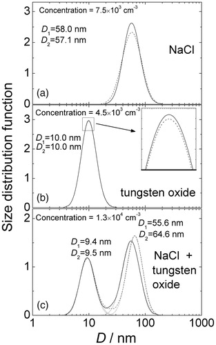
To measure the nanoaerosol number concentration and size distribution, the aerosol diffusion battery as described in Section 2 is used, coupled with a CPC counter (see in more detail Onischuk et al. 2018). To produce the laboratory aerosol of NaCl, a horizontal evaporation–nucleation flow generator is used (Onischuk et al. 2018). It comprises a quartz tube (inner diameter of 1.0 cm) with an outer oven. A flow of filtered air is supplied to the inlet with the rate of 15.0 cm³/s (under standard conditions). The maternal substance of NaCl is charged inside the tube to the middle of the hot zone to produce vapor. At the outlet of the hot zone, the vapor is mixed with cold air (supplied with a flow rate of 3.0 cm³/s). In the mixture zone, vapor becomes oversaturated due to the temperature decrease. As a result, aerosol is formed due to homogeneous nucleation followed by vapor to particles condensation and coagulation. The heating temperature in these experiments was within the range 750–1000 K. The typical particle number concentration at the outlet of generator and the mean diameter were in the ranges 10⁴–10⁷ cm⁻³ and 5–120 nm, respectively. To generate two-component aerosol, we used an additional source, which was a hot-wire tungsten oxide aerosol generator (Onischuk et al. 2018). The mean diameter and particle number concentration were in the ranges 5–20 nm and 10⁴–10⁷ cm⁻³, respectively. When measuring the aerosol spectra with the diffusion battery, aerosol concentration was kept in the range 10³–10⁵ cm⁻³ using an aerosol diluter. To compare the diffusion battery spectra with independent measurements, a JEM 100SX transmission electron microscope (TEM) was used. Sampling for TEM was conducted thermophoretically, using a copper electron microscopy grids covered with polyvinyl formal film. The comparison of NaCl particle size distributions as determined from the elaboration of TEM images (see Onischuk et al. 2018 for more detail) and diffusion battery measurements is given in the online SI (Figure S3). It was found that the arithmetic mean diameters, as determined from TEM and the diffusion battery, agree with each other within an accuracy of 10%, which is considered as the typical experimental accuracy. Figure S3 demonstrates the corrected solutions 1 and 2, however, in all DB measurements of single-mode spectra, there was no significant difference between corrected and non-corrected solutions.

To measure the spectrum of two-component aerosol, two aerosol flows were organized in parallel. The schematic of the experimental set-up can be found in the online SI (Figure S4). During the experiment, one of the flows passed through an aerosol filter, and the other one bypassed the filter. Then the single-component spectrum was measured. In the other case, both flows bypassed the filters, and then the two-component spectrum was measured. The concentration of the two-component aerosol is to be equal to the sum of single-component concentrations. The spectra of single- and two-component aerosols are demonstrated in Figures 4a–c. The original size spectra of the NaCl and tungsten oxide aerosols are shown in Figures 4a–c demonstrates the spectrum of the mixture of two aerosols. One can see that within the accuracy of 10%, the mixture concentration 1.3 × 10⁴ cm⁻³ is equal to the sum of original concentrations 7.5 × 10⁴ cm⁻³ and 4.5 × 10⁴ cm⁻³ of NaCl and tungsten oxide aerosols, respectively. The geometric mean diameters as determined from solutions 1 and 2 (corrected spectra) are given as D₁ and D₂, respectively. Within the accuracy of 2% solutions 1 and 2 gave the same mean diameters for the single-mode spectra. In a mixture spectrum, two components are well resolved. Spectrum components were fitted by lognormal functions (dotted lines). The geometric mean diameters for fitted functions are given in Figure 4c as D₁ and D₂ for solutions 1 and 2, respectively. One can see that the geometric mean diameters for the fitted functions agree within the accuracy of 10% with mean diameters for the original one-component spectra. The ratio of small-size to large-size peak intensities I_9nm/I_60nm = 0.7 in the mixture spectrum is in good agreement with the ratio of the original single-mode concentrations C_10nm/C_58nm = 0.6. Thus, both solutions resolve the experimental two-component spectrum well.

Figure 4. Particle size distributions retrieved from diffusion battery measurements (corrected solutions) for aerosol of NaCl (a), tungsten oxide (b), and mixture NaCl + tungsten oxide (c). Solid line – solution 1, dash line – solution 2, dot lines are lognormal fittings of two-mode spectra components. D₁ and D₂ are geometric mean diameters for single-mode spectra (a and b) and for the components of two-mode spectra (c) for the solutions 1 and 2, respectively.

7. Conclusions

In this article, the method of analytical inversion for the aerosol diffusion battery is further developed. The idea of the method arises from the fact that the diffusion battery divides the particles into groups (fractions), according to diffusivity, collecting them in different sections filled by stacks of screens. If one knows the size distributions of particles in fractions, then the original spectrum can be obtained as the sum of the spectra of fractions.

In this article, two different approaches are discussed giving analytical formulas to retrieve the mean diameters for particles in different fractions using the diffusion battery penetrations as input parameters. One of the approaches (solution 2) was partly discussed in our previous publication (Onischuk et al. 2018), and another one (solution 1) is quite new. Then, the spectra of fractions are approximated by lognormal functions using mean diameters obtained and the standard geometric deviation σ = 1.35. The final spectrum is approximated as the sum of lognormal functions with weights proportional to the number of particles separated by the diffusion battery sections.

The analytical solutions gave excellent results in the retrieval of single-mode spectra from the diffusion battery penetrations. However, in the case of two-mode spectra, the peak resolution can be poor for the nearby modes. This is mostly due to the ranges of diffusivity of particles collected by different DB sections overlap with each other, and, therefore, different modes from the original spectrum contribute to the same fractions of particles. To increase the resolution, the procedure of spectrum correction was applied, demonstrating good peak separation.

Comparison of the diffusion battery measurements for the laboratory generated NaCl aerosol with the observation using Transmission Electron Microscopy (TEM) showed a good sizing accuracy for both solutions 1 and 2. The mean diameters from diffusion battery measurements accord with those from TEM within an accuracy of 10%. To demonstrate the spectrum resolution, two laboratory generated aerosols (tungsten oxide and NaCl with the mean diameters 10 and 60 nm, respectively) were mixed together. These two modes were ideally resolved in the spectrum of mixture measured by the diffusion battery.

Nomenclature
a	=	lower limit of integration size interval
b	=	upper limit of integration size interval
C0	=	particle number concentration measured at the inlet of diffusion battery (cm−3)
CC	=	Cunningham correction factor
Ci	=	particle number concentration measured downstream of the i-th section of diffusion battery (cm−3)
CPC	=	condensation particle counter
D	=	particle diameter (cm)
Df	=	particle diffusion coefficient (cm2/s)
Di	=	mean diameter of particles of the i-th DB fraction
DB	=	diffusion battery
f(D)	=	particle size distribution function
	=	particle size distribution approximated by the sum of lognormal functions
gi	=	Ci/C0: penetration through the first i sections of diffusion battery
h	=	thickness of screen (cm)
h1, h2, …, hm	=	fractions of particles separated by diffusion battery
i	=	number of the diffusion battery section
Ki(D)	=	kernel function for the diffusion battery
k	=	Boltzmann constant (erg/K)
m	=	number of DB sections
nk	=	number of screens in the k-th section of diffusion battery
N1,i	=	total number of screens in the series of DB sections from 1 to i
Nl,l+s	=	nl + nl+1 + … + nl+s: total number of screens in the series of DB sections from l to l+s
	=	Peclet number
	=	penetration through a cascade of sections 1, 2, …, i for monodisperse particles of diameter D
	=	penetration through a stack of N screens for particles with size distribution φi
	=	interception parameter
r	=	radius of fiber in the screen (cm)
SGD	=	standard geometric deviation
T	=	absolute temperature (K)
U0	=	velocity of undisturbed flow through the diffusion battery (cm/s)
α	=	screen solid volume fraction
εi	=	experimental error for the penetration gi
	=	size distribution function for particles penetrated through the i-th DB section
η	=	gas dynamic viscosity (Poise)
λ	=	gas mean free pass (cm)
μ	=	single-fiber collection efficiency
μD	=	single-fiber collection efficiency due to diffusion
μDR	=	correction term for single-fiber collection efficiency due to interception for the diffusing particles
	=	mean single-fiber collection efficiency in a stack of N screens for particles coming out of the j-th section of diffusion batter
μR	=	single-fiber collection efficiency for interception
	=	mean single-fiber collection efficiency in a stack of N screens for the particles with size distribution function φi.
σ	=	standard geometric deviation
	=	size spectra of the fractions of particles separated by diffusion battery
	=	lognormal approximation of spectrum φi
	=	screen shape factor in the equation for aerosol penetration probability

Additional information

Funding

The reported study was funded by RFBR according to the research project No 17-43-540767 р_а.

References

- Amaral, S. S., de Carvalho, J. A., Costa, M. A. M., and Pinheiro, C. (2015) An Overview of Particulate Matter Measurement Instruments. Atmosphere, 6:1327–1345.
- Cheng, Y. S. and Yeh, H. C. (1980) Theory of a Screen-type Diffusion Battery. J. Aerosol Sci., 11, 313–320.
- Cheng, Y. S. Keating, J. A., and Kanapilly, G. M. (1980) Theory and Calibration of a Screen-type Diffusion Battery. J. Aerosol Sci., 11:549–556.
- Cheng, Y. S. Yeh, H. C., and Brinsko, K. J. (1985) Use of Wire Screens as a Fan Model Filter. Aerosol Sci. Technol., 4:165–174.
- Chow, J. C. (1995) Measurement Methods to Determine Compliance with Ambient Air Quality Standards for Suspended Particles. J. Air Waste Manag. Assoc., 45:320–382.
- Colbeck, I. (1995) Particle Emission from Outdoor and Indoor Sources in Airbome Particulate Matter, T. Kouimtzis, and C. Samara, Eds., Springer-Verlag, Berlin, 1–34.
- Crump, J. G., and Seinfeld, J. H. (1982) Further Results on Inversion of Aerosol Size Distribution Data: Higher-Order Sobolev Spaces and Constraints. Aerosol Sci. Technol., 1:363–369.
- Flagan, R. C. (2011) Electrical Mobility Methods for Submicrometer Particle Characterization, in Aerosol Measurement. Principles, Techniques, and Applications, P. Kulkarni, P. A. Baron, and K. Willeke, eds., Willey, New Jersey, pp. 339–364.
- Fuchs, N. A. The Mechanics of Aerosols. Pergemon Press: Oxford, 1964.
- Gevorkyan, E., Sofronov, D., Lavrynenko, S. and Rucki, M. (2017) Synthesis of Nanopowders and Consolidation of Nanoceramics of Various Applications. J. Adv. Nanomater., 2:153–159.
- Giechaskiel, B., Maricq, M., Ntziachristos, L., Dardiotis, C., Wang, X., Axmann, H., Bergmann, A., and Schindler, W. (2014) Review of Motor Vehicle Particulate Emissions Sampling and Measurement: From Smoke and Filter Mass to Particle Number. J. Aerosol Sci., 67:48–86.
- Guo, J., Fan, X., Dolbec, R., Xue, S., Jurewicz, J., and Boulos M. (2010) Development of Nanopowder Synthesis Using Induction Plasma. Plasma Sci. Technol., 12:188–199.
- Harrison, R. M. (1986) Analysis of Particulate Pollutants, in Handbook of Air Pollution Analysis, R. M. Harrison and R. Perry, eds., Chapman and Hall, New York, 155–214.
- Hunt, B., Thajudeen, T., and Hogan, C. J. Jr. (2014) The Single-Fiber Collision Rate and Filtration Efficiency for Nanoparticles I: The First-Passage Time Calculation Approach. Aerosol Sci. Technol., 48:875–885.
- Kirsch, A.A., Stechkina, I.B., and Fuchs, N.A. (1969). Studies on Fibrous Aerosol Filters—Experimental Determination of Fibrous Filters Efficiency in the Range of Maximum Particle Penetration. Colloid J. USSR 31:227–232.
- Knutson, E. O. (1999) History of Diffusion Batteries in Aerosol Measurements. Aerosol Sci. Technol., 31:83–128.
- Onischuk, A. A., Tolstikova, T. G., An’kov, S. V., Baklanov, A. M., Valiulin, S. V., Khvostov, M. V., Sorokina, I. V., Dultseva, G. G., and Zhukova N. A. (2016) Ibuprofen, Indomethacin and Diclofenac Sodium Nanoaerosol: Generation, Inhalation Delivery and Biological Effects in Mice and Rats. J. Aer. Sci., 100:164–177.
- Onischuk, A. A., Tolstikova, T. G., Baklanov, A. M., Khvostov, M. V., Sorokina, I. V., Zhukova N. A., An’kov, Borovkova, O. V., S. V., Dultseva, G. G., Boldyrev, V. V., Fomin, V. M., and Huang, G.S. (2014) Generation, Inhalation Delivery and Anti-Hypertensive Effect of Nisoldipine Nanoaerosol. J. Aer. Sci., 78:41–54.
- Onischuk, A. A., Baklanov, A. M., Valiulin S. V., Moiseenko, P. P., and Mitrochenko, V. G. (2018) Aerosol Diffusion Battery: The Retrieval of Particle Size Distribution with the Help of Analytical Formulas. Aerosol Sci. Technol., 52:165–181.
- Phillips, D. L. (1962) A Technique for the Numerical Solution of Certain Integral Equations of the First Kind, J. Assoc. Comput. Mach., 9: 84–97.
- Powell, M. J., Potter, D. B., Wilson, R. L., Darr, J. A., Parkin, I. P., and Carmalt, C. J. (2017) Scaling Aerosol Assisted Chemical Vapour Deposition: Exploring the Relationship Between Growth Rate and Film Properties. Mater. Des., 129:116–124.
- Reist, P. C. (1993) Aerosol Science and Technology, McGraw-Hill Inc., New York.
- Twomey, S. (1965) The Application of Numerical Filtering to the Solution of Integral Equations Encountered in Indirect Sensing Measurements. J. Franklin Inst., 279:95–109.
- Yeh, H.-C., and Liu, B. Y. H. (1974) Aerosol Filtration by Fibrous Filters–I. Theoretical. J. Aerosol Sci., 5:191–204.