Effect of particle charge on aerosol dynamics in Teflon environmental chambers

Abstract

The contribution of particle charge to the rate of particle wall deposition has been a persistent source of uncertainty for experiments performed in environmental chambers. By tracking the preferential deposition of positively charged particles; by comparing experiments carried out under standard, humid, and highly statically charged conditions; and by performing two-parameter optimizations for the chamber eddy-diffusion coefficient (k_e) and the average magnitude of the electric field (), the effect of charge on the rate of particle-wall deposition is isolated. A combined experimental and computational method is also developed for determining values for k_e and within a FEP Teflon chamber. To fully account for the effects of charge on particle dynamics in environmental chambers, studies of the effect of air ion concentration on the rate of particle coagulation over a typical 20 h experiment are performed and demonstrated, in general, that particle charge is negligible for characteristic chamber ion concentrations. While the effect of particle charge on aerosol dynamics in an environmental chamber must be addressed for each specific chamber, we demonstrate experimentally that for the Caltech 19 m³ Environmental Chamber, charge effects on the rate of particle-wall deposition are negligible.

Copyright © 2018 American Association for Aerosol Research

EDITOR:

• Nicole Riemer

1. Introduction

Data from environmental chambers are instrumental to understanding the chemistry of the atmosphere and aerosol formation. A common experiment in atmospheric chambers involves determination of the secondary organic aerosol (SOA) yield, the ratio of the mass of aerosol formed to that of a precursor vapor reacted. SOA yields are determined predominantly from experiments carried out in Teflon chambers. Since measurements of the amount of aerosol formed in such an experiment can be carried out only on suspended particles, one must account for particles deposited onto the chamber walls throughout the duration of an experiment to obtain an accurate assessment of SOA yield.

Particle charge has long been recognized as a possible factor in the rate of particle-wall deposition. McMurry and Rader (1985) determined empirical parameters describing the rate of wall deposition of charged particles by extrapolating the average electric field () from a small Teflon bag to a much larger chamber, obtaining a characteristic value of ∼45 V cm^–1. Since 1985, however, experimental chamber procedures have evolved, but questions of the strength of the average electric field in standard Teflon environmental chambers have remained. Currently, chambers are constructed so as to avoid the build-up of static charge on the walls. While it has long been assumed that some electric field remains within a Teflon chamber, the strength of the field or of its effect on particle wall deposition is largely unknown (Pierce et al. 2008; Nah et al. 2017; Tian et al. 2017).

In this article, we explore the effect of particle charge on aerosol-formation and aerosol-growth experiments carried out in Teflon-walled environmental chambers. Particle charge can influence both the rate of particle-wall deposition and the rate of particle-particle coagulation. Theoretical treatments of particle-wall deposition (Crump and Seinfeld 1981; McMurry and Rader 1985) and of the effect of particle charge on the rate of coagulation (Seinfeld and Pandis 2016, 562–565) exist. We present here a combined experimental-modeling study of the effect of charge on particle dynamics in a Teflon-walled environmental chamber with the goal of providing guidance as to its potential importance in chamber experiments.

We began with derivations of the effect of particle charge on coagulation rates and of the effect of a statically charged wall on the rate of particle-wall deposition. Then, we investigated the effects of charge and air ion concentration on coagulation using a dynamic chamber model. Next, we probed the strength of the mean electric field and its effect on wall deposition with three methods: (1) an experimental procedure that tracks positive charges, (2) a related experimental procedures that compares particle-wall deposition for a chamber operated under standard and humid conditions, and (3) an optimization method that relies upon the prior experiments and the chamber model previously used for coagulation. Finally, we discussed those effects that can be neglected.

2. Theory of charge effects on particle dynamics in Teflon chambers

2.1. Effect of particle charge on coagulation

As experiments to determine the rate of particle-wall deposition are performed, the number concentration of the non-volatile particles in the chamber is measured as a function of time. Since coagulation decreases the number concentration throughout these experiments, particles in each size bin are subject to both wall deposition and coagulation (Nah et al. 2017). Moreover, it is necessary to account for the dynamics of particles in each size bin, since the rate of particle deposition to the wall is dependent on particle size.

In theory, the rate of coagulation is affected by the presence of particle charge. Indeed, calculations reported by Ghosh et al. (2017) indicate that charging particles significantly beyond their steady-state charge distribution leads to a demonstrable effect on their rate of coagulation. However, approximations cited by Seinfeld and Pandis (2016, 562–565) indicate this effect for atmospheric aerosols are small.

For two particles with charge numbers n₁ and n₂ and diameters and , respectively, the Brownian coagulation kernel was adjusted by a factor of [1] to account for coulomb forces, where , is the dielectric constant of air, and is the permittivity of free space (Seinfeld and Pandis 2016, 562–565). Unlike Ghosh et al. (2017), we ignored electrostatic dispersion effects because, while charges are present, they should not be far from the steady-state bipolar charge distribution and there should not be significantly more charges of one polarity than of the other.

2.2. Effect of particle charge on wall deposition

Assuming symmetry of the wall deposition of positively and negatively charged particles, McMurry and Rader (1985) developed the following equation for the first-order particle-wall-deposition coefficient of particles that carry an average of n charges in a spherical chamber in the presence of an average electric field : [2] where k_e is the chamber eddy-diffusion coefficient, D is the particle Brownian diffusivity; R is the spherical equivalent radius of the chamber; D₁ is the first-order Debye function, defined as [3]

The terminal particle settling velocity is given by: [4] where ρ is the density of the particle, g is the gravitational constant, C_C is the Cunningham slip-correction factor, and μ is the viscosity of air (Seinfeld and Pandis 2016, 371–375). The magnitude of the electrostatic migration velocity, , where e is the elementary charge, is [5]

D is given by the slip-corrected Stokes-Einstein-Sutherland relation: [6] where k is the Boltzmann constant and T is the chamber temperature. The Cunningham slip-correction factor is: [7] where λ is the mean free path of air equal to , p is pressure within the chamber, R is the ideal gas constant, and MW_air is the molecular weight of air (Seinfeld and Pandis 2016, 371–375).

When the particle charge distribution (i.e., the number concentration of particles in each size interval with a given charge number) is known, the remaining parameters to be determined are the chamber eddy-diffusion coefficient, k_e, and the average electric field within the chamber, . Since neither k_e nor can be easily and reliably measured, these parameters must be determined by optimal fitting of experimental data.

3. Dynamic chamber model

A particle-mass-conserving computational model accounts for the effects of coagulation and particle-wall deposition due to Brownian motion and to electrostatic effects. The model is based on the numerical solution of the aerosol dynamic equation (Sunol et al. 2018). For all simulations except those involving small air ions, numerical solutions are obtained over 40 fixed-particle-size bins with mean diameters extending from 23 to 804 nm (chosen to match the range of the SMPS); when ions are considered (Section 4), 80 fixed-particle-size bins with mean diameters from 1.6 to 1631 nm are used. In both cases, these size bins are further differentiated into 13 charge bins, ranging from −6 to 6 elementary charges. Since particles in the size range typical of chamber experiments tend not to be highly charged, any particle predicted to have charges outside the range −6e to 6e are assumed to have saturated at −6e or 6e, respectively. Any positive or negative ions added are placed into the 1.6 nm diameter +1e or −1e bins, respectively. When the ion concentration is held constant, the values in these bins are not changed for the duration of the simulation; when the ion concentration is only an initial value, the particles in the 1.6 nm +1e and −1e bins are not replenished throughout the experiment. For calculations comparing number or surface area concentrations between cases with and without ions present, only particles with diameters above 20 nm are compared. All particles used in the particle-wall-deposition experiments, to be described subsequently, are non-volatile. Parameter values and variables are given in Table 1.

Table 1. Chamber and particle parameters.

Parameter	Symbol	Value
General
Boltzmann constant	k	1.38 × 10^–23 J K^–1
Dielectric constant of air	ϵ	1.0005
Elementary charge	e	1.602 × 10^–19 C
Gravitational constant	g	9.8 kg m^–1 s^–1
Molecular weight of air	MWair	29.0 g mol^–1
Particle density	ρ	1700 kg m^–3
Permittivity of free space	ϵ0	8.854 × 10^–12 F m^–1
Viscosity of air	μ	1.81 × 10^–5 kg m^–1 s^–1
Caltech chamber parameters
Pressure	p	745 Torr
Temperature	T	19.6°C
Volume of chamber	V	19.0 m^3
Definitions of variables
Average electric field within the chamber
Brownian diffusivity of a particle	D
Cunningham slip-correction factor	CC
Diameter (general)	Dp
Diameter of particle i	Dpi
Eddy-diffusion coefficient	ke
Electrostatic migration velocity
Elementary charges on particle i	ni
Equivalent radius of the chamber	R
Mean free path of air	λ
Optimization function	J
Particle number concentration	N
Positively charged particles directly from the chamber
Positively charged particles that are charge-conditioned
Particle surface area concentration	SA
Particle-wall-deposition coefficient (general)
Particle-wall-deposition coefficient with n charges
Terminal particle settling velocity	νs

As the particle population undergoes wall deposition, coagulation occurs continuously in the chamber. It is assumed that each coagulation event results in a new particle with a mass that is the sum of the masses of the two colliding particles and a charge equal to the sum of the charges of the two particles. Suspended particles are assumed to maintain their charge.

To perform these simulations, we assume an initial charge distribution. In typical environmental chamber experiments, aerosols are injected into the chamber and allowed to mix prior to the beginning of data collection. It is a standard procedure to use a neutralizer, also called a charge conditioner, to establish a particle charge distribution immediately after particle generation. The neutralizer upstream of the chamber contains a soft x-ray source that produces a charge distribution that is a function of particle diameter. By comparing the distribution of particles that flow through the upstream neutralizer in the presence and absence of a downstream, polonium neutralizer, we confirmed that the outputs from the two neutralizers are the same and, therefore, likely close to the charge distribution given by Wiedensohler (1988); however, the particles may not be at their steady-state distribution at the beginning of the experiment if is large or if a significant number of ions is present. Nevertheless, we assume a charge distribution computed with the Wiedensohler (1988) formula and provided in Table 1-1 of TSI (2013, 1–2).

The form of the particle-wall-deposition function depends, in principle, on the geometry of the chamber. As chambers with flexible walls are generally neither perfect spheres nor perfect cubes, we carried out the optimization procedure for these two limiting shape assumptions: for the spherical chamber, the equivalent radius is ; for the cubic chamber, the characteristic length is , where V is the volume of the chamber. Assuming the absence of an electric field () and focusing on experiments performed under standard operating conditions (“A”–“F”), optimal values of k_e were determined by minimizing J, as defined subsequently by Equation (8)[8] , for the spherical chamber assumption and according to the derived from Crump and Seinfeld (1981) for the cubic chamber. Figure 1 shows a comparison of the results of the two minimizations to the total measured number concentration; Figure 2 compares the optimal wall-deposition curves obtained for the two chamber shape assumptions. In each case, a negligible difference exists between the results based on the two limiting chamber shapes. We, therefore, confidently used the spherical assumption for the duration of this work.

Figure 1. Aerosol number concentration evolution for the six “Standard” experiments (Table 3), as compared to a computational model that assumes the 19.0 m³ chamber is spherical (dark gray/red) or cubic (light gray/blue). As model predictions are compared to data, the simulated number concentrations include contributions from coagulation and from wall deposition. The parameter k_e, which represents the effect of turbulent mixing in the chamber on the rate of particle wall deposition, was found through the optimization procedure described in the text, where particle charge is neglected (). The optimized results for a spherical and a cubic chamber are essentially identical.

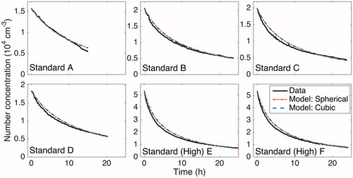
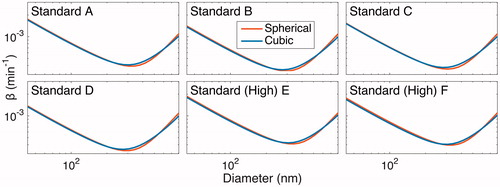
Figure 2. The size-dependent, wall-deposition parameter for a spherical (dashed, dark gray/red) and a cubic (light gray/blue) chamber of the same volume are compared for the six experiments performed under standard operating conditions. These curves were determined by minimizing J with respect to k_e (see Section 5.4), thereby fitting observations to simulated predictions. It was assumed that neither an electric field () nor any air ions were present. Due to the similarity of these curves, it is sufficient to represent the chamber as a sphere in this work.

4. Coagulation: Effect of charge and ions

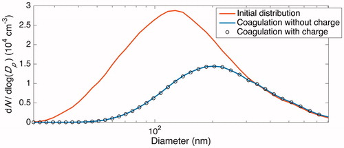
Using the Brownian coagulation kernel with the factor given in Equation (1)[1] and neglecting, for the moment, particle-wall deposition (setting for all diameters and all charges), we simulated a 20 h experiment with an initial number concentration of 2.1 × 10⁴ cm⁻³ and a distribution corresponding to the beginning of an experiment described in Section 5.3 (“Standard B”) with either uncharged particles or those having an initial charge distribution corresponding to the Wiedensohler formula. The final predicted number concentrations for the two cases are within 0.4% of one another (Figure 3).

Figure 3. Simulated number-concentration size distributions in the presence of coagulation only (no wall deposition) after 20 h. The initial distribution, shown in solid black/red, matches the initial condition for the “Standard B” experiment and has a total number concentration of ∼2 × 10⁴ cm⁻³. Simulations were performed both under the assumption that particles have no initial charge (gray line/blue line) and with the assumption that the initial charge distribution satisfies the Wiedensohler formula (circles/black circles). Since the size distributions under these assumptions coincide almost exactly (number concentrations are <0.4% different), one can conclude that the effect of particle charge on the rate of coagulation is negligible for chamber experiments similar to those considered here when there are no ions present.

In any laboratory, there are naturally occurring small air ions, also called cluster ions. These originate from, amongst other sources, galactic cosmic rays, radon decay in soil, splashing water, and nearby power lines (Hirsikko et al. 2011). While charge effects on coagulation may be negligible when particles are close to their steady-state charge distribution, this may not be the case in a standard laboratory setting.

To simulate the presence of ions, we assumed the ions to be particles with a diameter of 1.6 nm and a unit positive or negative charge. This diameter was chosen based on the size at which small air ions are defined by Hirsikko et al. (2011), but it is only an approximation, since different ion polarities may have different mobilities or diameters depending on the environment. Here, we consider only small air ions because ions larger than cluster ions are not produced within a chamber. We have verified, for example, that Caltech Environmental Chamber experiments are clear of particles of 1.7 nm diameter (personal communication, H. Mai, March 2018).

Simulated 1.6 nm ions at a chosen concentration were added to the initial distribution corresponding to that of the “Standard B” experiment. Then, in the absence of wall deposition, we allow the particles and ions to coagulate for 20 h. We consider ion concentrations between 0 and 5000 cm⁻³ at different polarity ratios, noting that 5000 cm⁻³ per polarity is an extreme ambient ion concentration (Vartiainen et al. 2007; Hirsikko et al. 2011). Adding these particles to the simulation increases particle volume in the chamber by <0.01%. Particle volume is, therefore, still considered conserved in the absence of wall deposition.

When we consider ions, we account for the presence of charge in the coagulation calculations. In order to determine the extent to which charge effects can be neglected, we must compare the result of these simulations to ones that do not account for a charge or for ions, which we call the Reference Case. Relative charges in the total aerosol number or surface area concentrations after 20 h of simulated coagulation are compared to what those concentrations would have been in the absence of ions and of charge (the Reference Case).

Even when the ion concentrations are high and are held constant, the effect of charge on coagulation is minimal for equal concentrations of positive and negative ions, as shown in Case 5 (Figures 4 and 5, Table 2): there is only a 0.88% difference in number concentrations after 20 h between the Reference Case and a simulation with positive and negative ion concentrations of 5000 cm⁻³ each. In the absence of an ion production source, i.e., when there is no maintaining of the ion concentration and if the ion concentration is not held constant, the charge effect on the rate of coagulation is also negligible (Cases 6 and 7).

Figure 4. Total number and surface area concentrations after 20 h of coagulation (neglecting wall deposition) at different ion concentrations according to the 7 cases described in Table 2 are shown in panels (a) and (b), respectively. The initial number concentration and surface area concentration of 2.0 × 10⁴ cm^–3 and 2.8 × 10³ µm² cm^–3 are displayed as the top dashed line in these panels. These concentrations – excluding the variable concentration of ions present – correspond to the initial condition for the simulations taken from the initial particle distribution of the “Standard B” experiment, which is shown in solid black/red in Figure 3. The final number and surface area concentrations when no ions are present and each particle has a neutral charge (the Reference Case), shown as the bottom dashed line in the same panels, are 9.2 × 10³ cm^–3 and 2.4 × 10³ µm² cm^–3; the percent difference of the final number and surface area concentrations from these values are shown in panels (c) and (d), respectively. When there is a large difference between the concentrations of the two ion polarities (Case 1–3), the rate of coagulation is dramatically decreased and, therefore, the difference between the coagulated concentrations with and without considering ions and charge is fairly significant. When the difference in concentrations of the two ion polarities are maintained but the absolute concentrations increase, the difference from the Reference Case decreases (Case 4 and Cases 1–3 for the same x). Values for Cases 4 through 7 are shown more clearly in Figure 5.

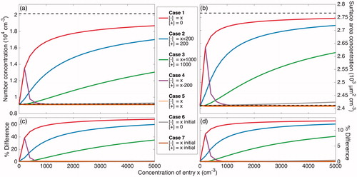
Figure 5. A magnified version of Figure 4 that more clearly displays Cases 4 through 7 (defined in Table 2). Panels (a) and (b) show the total simulated number and surface area concentrations after 20 h of simulated coagulation. The initial distribution corresponds to the beginning of the experiment “Standard B,” but with ions present. In panels (c) and (d), the final number and surface area concentrations for Case 4 through 7 are compared to 9.2 × 10³ cm^–3 and 2.4 × 10³ µm² cm^–3, which are the final total number and surface area concentrations for the Reference Case. When no ion production source is present, as approximated in Cases 6 and 7, there is a negligible effect of the ion concentrations and of charge on coagulation. Even for high ion concentrations, when the two polarities are of equal concentrations (Case 5), there is a small effect of charge. Only when there is a difference between the positive and negative ion concentrations (Cases 1 through and 3), does much of an effect of charge exist. When the difference between the two polarity concentrations remains constant, the effect of charge on coagulation decreases as the absolute concentrations of ions increases (Case 4).

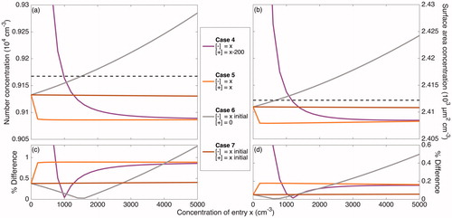
Table 2. Coagulation of the “Standard B” initial particle size distribution with 1.6 nm diameter ions over 20 h.

Case	Description	Negative ion concentration (cm	Positive ion concentration (cm	Held constant?	% Difference of number concentration at x equal to		% Difference of surface area concentration at x equal to
					200 cm^–3	5000 cm^–3	200 cm^–3	5000 cm^–3
1	[−] varies, [+] = 0	x	0	Yes	38%	68%	8.8%	13%
2	[−] varies, [+] = 200	x + 200	200	Yes	0.88%	59%	0.18%	12%
3	[−] varies, [+] = 1000	x + 1000	1000	Yes	0.32%	35%	0.014%	8.1%
4	[+] – [-] = 200	x	x−200	Yes	38%	0.86%	8.8%	0.15%
5	[−] = [+]	x	x	Yes	0.88%	0.89%	0.18%	0.16%
6	[−] varies, [+] = 0	x	0	No	0.34%	1.3%	0.037%	0.50%
7	[−]= [+]	x	x	No	0.38%	0.40%	0.051%	0.057%

Wall deposition was neglected ( = 0 for all diameters and all charges). Entry x in the table varies from 0 to 5000 cm^–3 (except for when this leads to a negative ion concentration). Percent differences were calculated as the difference between the number or surface area concentrations calculated after 20 h of the condition considered and the number and surface area concentrations of the Reference Case. The Reference Case is a 20 h simulation of coagulation where the ion concentrations are 0 and all particles are assumed to have a neutral charge: this gives a final number concentration of 9.2 × 10³ cm^–3 and a final surface area concentration of 2.4 × 10³ µm² cm^–3. If the concentration is not held constant (“no” for column “Held Constant?”), then ions are added at the beginning of the simulation only; if they are held constant, any ions that disappear by coagulation are replaced so that a constant ion concentration is maintained. Figures 4 and 5 show these values in graphical form.

However, holding the positive ion concentration constant while varying that of the negative ions leads to a significant effect of charge on coagulation, as given by Cases 1 through 3 (Figure 4, Table 2). Note that as the value of the constant positive ion concentration is increased, while maintaining the absolute difference in polarity concentrations, the final distributions found by assuming that only coagulation occurs approach that of the Reference Case. We see this when comparing Case 2 to 1 and Case 3 to 2. Case 4 shows this more directly; the absolute difference between ion polarity concentrations is maintained at 200 cm⁻³ as the concentrations increase.

In what are seemingly symmetric simulations, there is a slight difference when the concentrations of the ion polarities are switched (e.g., if we compare the case of positive ions at 200 cm⁻³ and negative ions at 0 cm⁻³ to the case of positive ions at 0 cm⁻³ and negative ions at 200 cm⁻³), because the Wiedensohler distribution exhibits a slight preference for negatively charged particles over positively charged ones. However, these differences are sufficiently small that we, simply and conservatively, report values for the simulation that, in general, gives a higher percent difference instead of reporting nearly identical simulations.

Ion production within the chamber by cosmic rays or other energetic particles result in ion pairs with negative charges initially present as free electrons that later attach to gas molecules. However, differing ion mobilities may lead to different ion polarity concentrations (Reiter 1985; Harrison and Aplin 2007; Hirsikko et al. 2011). Thus, while the ratio of positive and negative ions tends to be close to 1, it is not always exactly 1. Nonetheless, Hirsikko et al. (2007) found that, in an urban environment, the difference in concentration between positive and negative small air ions was minimal, both indoors and outdoors. For example, the median positive and negative ion concentrations indoors were 966 and 1065 cm⁻³ on a weekday and 1357 and 1376 cm⁻³ on a weekend, respectively. When we repeat the simulations described above with these ion concentrations, we find that the charge effect on coagulation rates is still minimal: a 0.72% and 0.13% difference indoors on weekdays in number and surface area concentrations, respectively. On the weekends, there is a 0.89% and 0.17% difference. Therefore, though charge can have a significant effect on the rate of coagulation, we do not expect it will for typical environmental chamber experiments.

5. Particle wall deposition: Effect of charge probed three ways

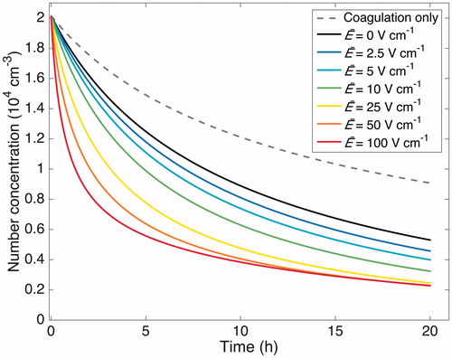
We turn now to the effect of charge on the rate of particle-wall deposition. Using the chamber model, Figure 6 shows the simulated effect of the average electric field () on the rate of particle-wall deposition. Both coagulation and wall deposition are accounted for; a simulation with coagulation alone is shown for comparison. Beginning with an initial distribution corresponding to that of an experiment described below (“Standard B”) and simulated for 20 h, values of  = 2.5 V cm⁻¹ and  = 100 V cm⁻¹ lead to final number concentrations that are 86% and 44%, respectively, of that when  = 0. Therefore, the presence of a surface charge will have an effect on particle wall deposition.

Figure 6. Simulated particle-number-concentration evolution subject to coagulation and wall deposition for a 20 h experiment. The initial number distribution matches that of the “Standard B” experiment (see Figure 3). The effect of assumed electric field strength is shown, based on s^–1. The results indicate that the strength of the electric field is influential, even when relatively small. The black curve shows the number concentration evolution in the absence of an electric field. The gray, dashed curve shows the sole contribution of coagulation to the particle-number-concentration evolution.

If there is a charge present on the walls of a Teflon chamber, it would likely be a negative charge because FEP Teflon film is often observed to be negatively charged and because PTFE Teflon, which is similar in structure to FEP Teflon, has been shown to have a large negative charge affinity (Sessler et al. 1992; Chen and Wang 2017). If there is no additional ion source, a negatively charged wall would lead to preferential depletion of the positively charged particles in the chamber. Since there are a finite number of positively charged ions, if one does not account for the electric field and simply attempts to determine , it would appear as if is a function of time.

If it can be shown that no electric field is present, then one can justify the use of a that is independent of time and is valid in multiple experiments. We provide here three methods for making this determination: the SMPS method, the humidity method, and the parameter optimization method. If one seeks to determine the extent to which an electric field exists in a laboratory chamber, we suggest the experiments and optimizations described below. If it is established that a chamber is free of surface charge, one need not account for a time-dependent . Alternatively, with these verification methods, one will be able to adjust the conditions of a chamber so that it does not exhibit an average electric field.

5.1. Experimental protocol

All particle dynamics experiments were performed in the Caltech 19 m³ Environmental Chamber that has 2 mil FEP Teflon walls. Before each experiment, the chamber is flushed with clean, dry air for >24 h, and contact with the chamber surface is minimized. Experimental conditions are summarized in Table 3. In “Humid” experiments, the chamber enclosure (the area outside of the environmental chamber) had a relative humidity of >40% at an average temperature of ∼20°C; for the rest of the experiments (“Standard” and “Static Charge”), the enclosure temperature was also ∼20°C but had a relative humidity <30% (usually ∼25%). For experiments that required a static charge (“Static Charge” experiments) on the chamber walls, charge was induced by rubbing cloth against the external walls prior to or during an experiment. While “Static Charge” experiments are characterized by a greater value of than either the “Standard” or the “Humid” experiments, the value of in an individual experiment likely varied due to the uncontrolled duration and vigor of charge inducement between or during experiments.

Table 3. Conditions for experiments performed.

Label	Relative humidity	Induced static charge?	Initial number concentration (cm^–3)	Initial surface area concentration (µm^2 cm^–3)	Experiment duration (h)
SMPS	<30%	Partway^a	3.4 × 10^4	3.5 × 10^3	4.1 + 2.2^b
Standard A	<30%	No	1.6 × 10^4	2.6 × 10^3	15.1
Standard B	<30%	No	2.1 × 10^4	2.7 × 10^3	23.7
Standard C	<30%	No	2.0 × 10^4	1.9 × 10^3	23.8
Standard D	<30%	No	1.8 × 10^4	2.4 × 10^3	20.3
Standard (High) E	<30%	No	5.3 × 10^4	6.6 × 10^3	25.1
Standard (High) F	<30%	No	5.4 × 10^4	7.0 × 10^3	24.2
Humid G	>40%	No	1.9 × 10^4	2.2 × 10^3	19.4
Humid H	>40%	No	3.0 × 10^4	3.5 × 10^3	17.0
Static charge I	<30%	Yes	1.8 × 10^4	1.9 × 10^3	23.9
Static charge J	<30%	Yes	1.3 × 10^4	1.8 × 10^3	23.2

^a In the “SMPS” experiment, a static charge was induced partway through the experiment.

^b The “SMPS” experiment began 4.1 h before a static charge was induced and then proceeded to run for an additional 2.2 h.

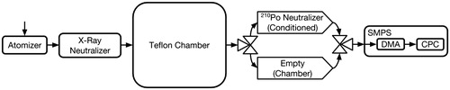
Experiments were performed over a range of initial particle concentrations (Table 3). Particles were injected into the chamber by atomizing an aqueous (NH₄)₂SO₄ solution at a flow rate of 2.6 L min^–1. In order to obtain a sufficiently broad size distribution, a 0.6 M solution was atomized for roughly half of the injection duration and a 0.006 M solution was atomized for the remaining time. After atomization, the particles were dried and then charge conditioned with a soft x-ray neutralizer (TSI Advanced Aerosol Neutralizer Model 3088) before entering the chamber. The injection time varied based on the desired initial chamber particle number concentration. After a few minutes of mixing, the time- and size-resolved number concentration in the chamber was recorded using a custom-built scanning mobility particle sizer (SMPS) comprised of a coupled differential mobility analyzer (DMA) employing recirculating flow, and a butanol-based condensation particle counter (CPC), models TSI 3081 and TSI 3010, respectively. The SMPS was operated with an aerosol flow rate of 0.515 L min^–1 and a 2.67 L min^–1 sheath and excess flow. Voltage scans (from 15 to 9850 V) were carried out with measurements made during a 240 s increasing voltage ramp. For experiments “A”–“J,” the aerosol flowed through a ²¹⁰Po source neutralizer prior to entering the DMA. For the “SMPS” experiment, the aerosol flow path was switched at the end of each scan between two pathways of nearly identical length and geometry, each of which led to the DMA after passing through a charge conditioner holder. One of these holders contained ²¹⁰Po sources, while the other did not (Figure 7). This made it possible to contrast measurements of the charge state in the chamber against that of a freshly neutralized aerosol.

Figure 7. Experimental setup for the scanning mobility particle sizer (SMPS) experiments to determine the ratio of positively charged particles of a specific electrical mobility actually in the chamber () to what the steady-state distribution of positively charged particles in the chamber would be (). Those that pass through the “Chamber” pathway are counted as , while those that pass through the “Conditioned” pathway are counted as . The SMPS comprises a differential mobility analyzer (DMA) and a condensation particle counter (CPC).

5.2. Wall deposition method 1: Using the SMPS

A scanning mobility particle sizer (SMPS) with a negative voltage source measures positive particles based on their electrical mobility, which increases with decreasing mass to charge (m/z) ratio. At the beginning of a voltage scan, particles with the largest mobility (smallest m/z ratio) successfully travel through a column and are then counted. As the voltage increases, the column selects for larger m/z ratios. Therefore, as the time into the voltage scan increases, the electrical mobility of the positively charged particles transmitted decreases.

Under general operation, in order to obtain the particle size distribution from SMPS data, aerosol is passed through a charge conditioner that produces a known, steady-state charge distribution before entering the DMA. Only a small fraction of the particles acquire charge, and so the concentrations of charged particles transmitted through the SMPS at a particular time in the scan is divided by the probability that a particle of the corresponding size has acquired a positive charge. That probability is estimated using the Wiedensohler (1988) charge distribution.

To determine the charge state of the aerosol within the chamber, we have added a second path for the aerosol to enter the DMA, as shown in Figure 7. This pathway is identical to the first one except that the ²¹⁰Po elements have been removed from the charge conditioner. Thus, the aerosol enters the DMA without altering the charge state from that within the chamber, while being subjected to the same losses within the instrument.

The differences between charge states obtained by these two methods can be seen by comparing the number of charged particles detected using the charge conditioner, , with that obtained directly from the chamber, . Unlike under general operation, no correction is made for the charging probability in this comparison as that for the latter () is unknown. In other words, is the concentration of positively charged particles in the chamber, while is the concentration of positively charged particles in the chamber if the particles within the chamber are in charge steady-state.

The standard notation of n⁺ is usually used to symbolize the particle number concentration per particle diameter and has units of number per volume per length (Seinfeld and Pandis 2016, 328–329). Since we cannot accurately convert from electrical mobility to particle diameter, we instead allude to the standard notation but use n⁺ to represent the number concentration of particles transmitted to the CPC integrated over 0.5 s of the voltage scan (20.5 V). Therefore, here the units of n⁺ are number per volume in 0.5 s of the voltage scan. Technically, then, n⁺ must be integrated over an electrical mobility range, not a diameter range, to get the total number of positively charged particles. However, since most positively charged particles of the sizes we consider will have no more than a single charge, electrical mobility is analogous to diameter. However, a decreasing electrical mobility corresponds to an increase in particle diameter. As a voltage ramp proceeds, the diameter of a singly charged particle that is counted by the CPC will increase.

For a specific voltage, if , then the charge distribution entering the SMPS system is close to the Wiedensohler distribution at the particle diameter generally corresponding to the electrical mobility transmitted at that voltage. If , more positive particles of that size exist than in the Wiedensohler distribution, and if , there are fewer. We, therefore, track .

More important than the exact value of is the extent to which this ratio is constant, since a constant ratio indicates the absence of forces acting preferentially on positively charged particles over negatively charged particles. That is, if is constant, there is no electric field effect on the rate of wall deposition and, therefore, is not a function of time.

Figure 8 shows the number concentration of positively charged particles that are passed through the charge-conditioned pathway (Panel (a), called “Conditioned”) and through a direct, non-neutralized pathway (Panel (b), called “Chamber”) shown in Figure 7. When the chamber is operated in a standard condition (−4.1 to 0 h), wall deposition and coagulation both gradually decrease the number concentration. Coagulation also shifts the peak in transmitted particles to a lower electrical mobility (for singly charged particles, to a larger diameter). Experimental conditions are shown in Table 3 (“SMPS”).

Figure 8. Concentration of positively charged particles that reach the CPC through the “Conditioned” (a) and through the “Chamber” (b) pathway, as shown in Figure 7. Both and have units of particle number per cm³ per 0.5 s of the voltage scan. The top axis labels the approximate diameter of transmitted singly and positively charged particles, found using analytical methods (Stolzenburg 1988). Since most, but not all, transmitted particles are singly charged, this corresponds only roughly to the size of the particles that reach the CPC. Prior to charge inducement, the chamber was run under standard operating conditions. After 4.1 h of operation, i.e., at 0 h, a static charge was induced on the chamber walls. The first scan after charge inducement is shown in bold. The curves in each panel are separated by 13 min except for those immediately after charge inducement: these are 6.5 min in panel (a) and 19.5 min in panel (b).

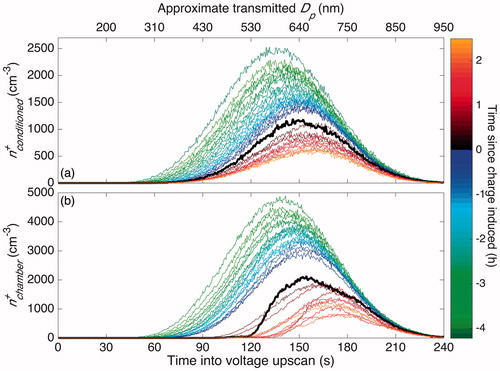
When a static charge is induced, positively charged particles with the highest electrical mobility disappear first. This matches intuition: if there is a large negative charge on the chamber walls, positively charged particles will be lost preferentially and the ones that will be lost most quickly are those with the highest electrical mobility.

In Figure 9, the ratio of positively charged particles that flow through an empty pathway to those that flow through the charge-conditioned pathway () is shown for the same experiment as in Figure 8. After a static charge was applied to the walls at 0 h, the ratio decreased rapidly, indicating that when the wall is charged, a preferential loss of positively charged particles does occur as expected. When the chamber was operating in a standard condition (−4.1 to 0 h), there was no change in , indicating that no charge was present on the chamber walls.

Figure 9. The absence or presence of an electric field within the chamber is discerned by the concentration of positively charged particles that are in the chamber at a given time () as compared to the concentration of positively charged particles from a charge-conditioned version of the same sample (). Since the same SMPS system was used to measure the concentrations from both pathways, the ratio is calculated as divided by the average of the two closest in time. Curves are, therefore, 13 min apart except for the curve immediately after charge inducement (shown in bold), which is 19.5 min apart from the previous one so as to give the most accurate ratio between the before and after inducement cases. As in Figure 8, the top axis shows the approximate diameter of transmitted singly and positively charged particles, which only inexactly corresponds to the size of the particles that reach the CPC.

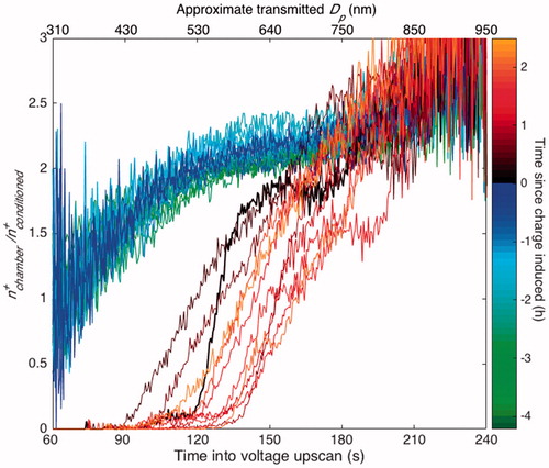
Immediately after charge inducement, the concentration of the smallest positively charged particles nearly disappears. Within about half an hour, there is still a preferential depletion of positively charged particles but the smallest ones begin reappearing. This is likely because of the air ions which, if there were no polar-preferential wall losses, would re-establish a steady charge distribution within this time frame (for characteristic ion concentrations). Since  < even 2 h after charge inducement, we conclude that the effects of the static charge on the chamber remain long after the charge is initially induced. While the discharge time likely depends on the initial strength of the electric field and on the concentration of air ions, we have observed static charges that remain for >8 h and we assume they remain for much longer.

As mentioned above, a constant is sufficient to establish that the rate of wall deposition is not dependent on the surface charge of the Teflon walls, which indicates that will not change with time. Intuitively, however, one would expect if the particles within the chamber are at their steady-state charge distribution. We see in Figure 9, however, that (this was confirmed in other, identical, standard experiments). This suggests that, either there is an unintended experimental difference between the two pathways, there is a preference for negatively charged particles to deposit to the wall, or the air ions are affecting this ratio.

We confirmed that the two pathways (“Conditioned” and “Chamber”) shown in Figure 7 have approximately the same transmission efficiency. We also confirmed that, when measured directly from the upstream x-ray neutralizer, . This indicates that particles that enter the chamber are at a steady-state charge distribution. If there is an electric field caused by a static charge on the chamber walls, we would expect it to be negatively charged because Teflon has a high negative-charge affinity, as discussed at the beginning of Section 5. A negatively charged wall would lead to the preferential loss of positively charged particles (not negatively charged particles, as we see here). So, it is unlikely that the presence of excess positively charged particles is a result of a surface charge on the Teflon walls.

The observed values of , then, can be attributed to air ions. When, in the absence of wall deposition, we simulate coagulation as described in Section 2.1, we compare simulations in the presence and absence of ions. For the same charge and diameter, in general, there were more positively charged particles when ions were present as long as the negative ion concentration did not greatly exceed the positive ion concentration. This was true even for cases in which the charge effects on the rate of coagulation were minimal. In the simulations, the time required to reach an approximately steady was less than the particle injection and mixing time. We conclude, then, that owing to the production of air ions with different properties than those generated in the charge conditioner; the conclusion from this experiment that charge does not alter the rate of wall deposition remains.

5.3. Wall deposition method 2: Humidity effects on static charge

The second method for determining the effect of charge on wall deposition relies on the assumption that, as the relative humidity of the air surrounding an environmental chamber increases, there is a corresponding decrease in the static charge on the chamber walls.

A study of the effect of humidity on the corona charging of polyvinylidenefluoride (PVDF) films, similar in structure to FEP Teflon, shows a linear decrease in the maximum voltage generated with an increase in relative humidity and, furthermore, that increasing the relative humidity decreases the surface potential even for a film that is already charged (Ribeiro et al. 1992). Ribeiro et al. (1992) postulate this is a result of dissociated absorbed water on the film surface.

According to Funer and James (1993), typically PVDF film shows an absorption of water of 0.02%, while polytetrafluorethylene (PTFE) Teflon shows an absorption of <0.01% water when immersed at 23 °C, which are both infinitesimally small. Another study of the amorphous version of PTFE films (Teflon AF) showed no measurable absorption of water until 75% relative humidity was reached (Vetelino et al. 1997). PTFE Teflon has fluoride atoms bound to carbon atoms; FEP Teflon has both fluoride atoms and trifluoromethyl groups bound to carbon atoms, whereas PVDF films consist of hydrogen and fluoride atoms bound to carbon atoms. Therefore, while it is possible that the relative humidity effect is unique to PVDF films, the Ribeiro et al. (1992) study suggests that it is possible, if not probable, that increasing the relative humidity surrounding a chamber will decrease the chamber’s surface charge.

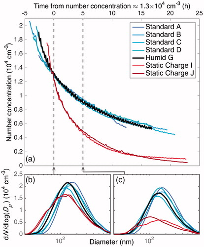
Figure 10a shows dynamics of the total number concentration of inorganic particles subject to simultaneous coagulation and wall deposition for experiments that began with approximately the same number distribution and are aligned at a common number concentration (as verified in the displayed size distribution in Figure 10b). The “Standard” experiments align with each other, as expected, but also with the “Humid” experiments. The “Static Charge” experiments, although they begin with approximately the same number concentration and size distribution, exhibit much faster wall deposition than either the “Standard” or the “Humid” experiments. The electric field on the chamber walls affects only wall deposition, so the sole difference between these experiments is the average electric field. Since the number concentration evolution in the “Standard” and the “Humid” experiments overlap, they likely are subject to the same ; Figure 10a verifies that the total number concentration evolutions align, and Figure 10c shows that the number distribution does as well.

Figure 10. Particle-number-concentration evolution for experiments with approximately the same initial number concentration and size distribution. For humid and standard conditions, the number-concentration evolutions overlap. When a static charge is present, wall deposition occurs much faster and the number concentration decreases more quickly (a). The particle size distribution aligned at a time when all the experiments shown have an approximate number concentration of 1.3 × 10⁴ cm^–3 (b) is compared to that distribution about 5 h later (c). All distributions begin similarly, but the particles under static charge conditions deposit much faster. Thus, the evolution in total number concentration, shown in panel (a), is not a result of the difference in the rate of coagulation or in the diameter-dependence of the wall-deposition rate. The difference in the number-concentration evolution, then, is a result only of the electric field strength. Since in a humid experiment, the static charge on the chamber walls is reduced, and therefore decreases any electric field that may be on the chamber, the similarity in wall-deposition rates between the “Humid” and “Standard” experiments indicates that any electric field present in the standard experiments has a negligible effect.

The number concentration evolution is sensitive to the electric field, as shown both from the number concentration evolution in Figure 6 and from the fact that an increase in static charge from the standard conditions does lead to an increase in the rate of wall deposition (demonstrated by the increase in deposition for the “Static Charge” experiments).

If higher humidity conditions do reduce the electric field strength, the “Humid” experiments should show less of a static charge on the chamber walls compared to the “Standard” experiments, if such a charge exists. Since the “Humid” experiment matches the “Standard” experiments, any difference in average electric fields can be considered to be negligible. Thus, since it is possible that any charge on the chamber walls would decrease when the enclosure is at a higher humidity, this is additional evidence that the charge on the chamber walls is negligibly small, even when operated under standard conditions.

5.4. Optimal parameter estimation

The basic experimental procedure to determine k_e and is centered on the measurement of the dynamics of the size distribution of particles introduced into the chamber. We compare the observed dynamics to those predicted by a numerical solution to the aerosol dynamics equation. The numerical solution includes contributions from coagulation and wall deposition, the latter in the form of undetermined parameters, k_e and , which govern the rate of particle-wall deposition owing to mixing in the chamber and to electrostatic effects, respectively.

Seemingly, a complicated optimization procedure could be avoided by directly measuring the electric field on a Teflon surface. However, it cannot be assumed that the electric field immediately adjacent to the Teflon walls is the same as the average electric field within the chamber (McMurry and Rader 1985). Moreover, neither nor k_e can be measured empirically. Therefore, both parameters must be determined by optimal fitting of time-dependent chamber particle-wall-deposition data.

The general optimization method is as follows: we begin with an initial size-resolved number concentration distribution that matches that from the first SMPS scan of the experiment considered, then we assign to it a charge distribution corresponding to the Wiedensohler (1988) formula, as detailed in Section 3. Next, we iteratively minimize the objective function J by determination of the parameters k_e and , where [8]

Note that when , particle charge is not a factor, and J is a function only of k_e. Minimization of J is performed with the Matlab fminsearch function, which uses a Nelder–Mead simplex algorithm (Lagarias et al. 1998).

5.5. Wall deposition method 3: Determining the electric field through optimization

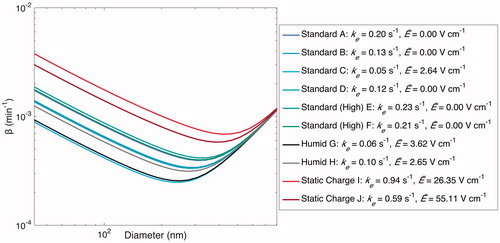
The final method for determining the charge effect on wall deposition rates has the additional benefit of providing necessary parameters for representing wall deposition, whether or not there is a static charge present on the chamber walls. We use the optimal parameter procedure from Section 5.4 and the experimental data from Section 5.3 to carry out an optimization simultaneously for k_e and for . The results are shown in Figure 11 and discussed below.

Figure 11. Optimal estimated based on the values of k_e and (given in the legend) when particles are assumed to have an initial charge. Optimized values of for the experiments performed under standard conditions are close to 0; those for the “Static Charge” experiments are much larger than those for the “Standard” and “Humid” experiments.

Determining an optimal value for k_e while assuming that there is a negligible electric field present on the chamber walls ( 0) is equivalent to assuming that the particles within the chamber are essentially charge-free. This is supported by the fact that coagulation is affected minimally by the presence of charge under characteristic indoor ion concentrations and, when  = 0, particle charge has no effect on the rate of wall deposition. When this optimization is carried out, the “Humid” and “Standard” experiments are characterized by similar k_e values and produce similar wall-deposition curves (as shown in Figure 12). This corroborates that the “Humid” and “Standard” experiments are nearly indistinguishable and, therefore, reflect nearly identical values.

Figure 12. Optimal estimated based on values of k_e when particles are assumed to be charge-free. Optimal values of k_e are shown in the legend. Note that particles within the chamber may have significant charge, but that this affects the -curve only when static charge is induced on the chamber walls prior to or during an experiment.

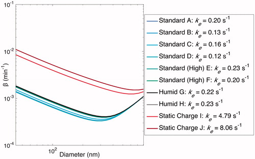
The “Static Charge” experiments, on the other hand, lead to very different curves and significantly larger k_e values. Since, for these experiments, , these larger optimal values of k_e, in effect, attempt to compensate for the charge contribution to wall deposition.

With a two-parameter optimization, small values for the “Humid” and “Standard” experiments are attained. Figure 11 shows the optimized k_e and values and the corresponding curves: is small for all but the “Static Charge” experiments. We show , which is the for particles with a charge of 0, because most particles are neutrally charged and so, when comparing wall-deposition rates, it is most informative to consider the wall-deposition rate of neutrally charged particles.

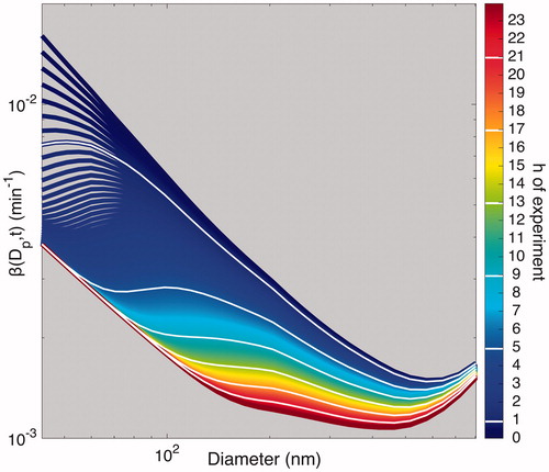
To demonstrate further that, when , there is an increased rate of wall deposition, especially for smaller particles, we include Figure 13, which is a transformation of to for the “Static Charge I” experiment. Figure 13 is similar to a figure in Pierce et al. (2008), which also shows that an electric field caused by surface charge affects the rate of wall deposition.

Figure 13. Transformation of to for the “Static I” experiment using the parameters optimized for that experiment (k_e = 0.94 s^–1 and  = 26.35 V cm^–1). was determined every 6.5 min. At the beginning of the experiment, is much larger than that towards the end of the experiment. This difference is particularly pronounced for small particles.

The fact that the majority of the “Standard” experiments (five of the six) lead to an optimal value of  = 0 further reinforces the essential absence of an electric field for experiments performed under the standard conditions.

6. Further optimization: Finding the empirical k_e parameter

Once one has verified the lack of a charge effect on the rate of particle wall deposition, one can reduce the optimization of the wall-deposition coefficient to one parameter. Note that the curves in Figure 11 are less tightly clustered than those in Figure 12 because a two-parameter fit allows a trade-off between the two parameters to account for the number concentration evolution, producing local minima instead of an absolute minimum.

If a local minimum is found, two possibilities exist: either the minimization procedure converged to a local minimum because of the initial guess chosen, or the data – which are subject to random error – give an absolute minimum at a point that (if the data are completely accurate) corresponds to what is actually a local minimum. To address the former possibility, we reanalyzed experiments “Standard C” and “Static Charge I” with initial guesses of k_e between 0.015 and 1.5 s^–1 and of between 5 and 500 V cm⁻¹. Each optimization returned the originally reported minimum.

Because of the trade-offs in parameter values, optimizing solely for k_e, while setting to 0, or optimizing for both parameters gives good agreement to the data; see Figures 14 and 15, where the former is shown in green, the latter is shown in blue, and data are shown in black. The wall-deposition curves for each experiment, which are similar for the “Standard” and “Humid” experiments but quite different for the static one, are shown in Figure 16.

Figure 14. Particle-number-concentration evolution throughout the duration of experiments under standard, humid, and static charge conditions. Data are compared to the simulated number concentration calculated with parameters found from different forms of optimization. Data are given in solid black, and a model with only coagulation included (no wall deposition) is the solid, light, gray curve shown to demonstrate that a significant amount of the loss in number concentration is the result of particle wall deposition. For experiments “A”–“H,” the final selected k_e and values of 0.19 s^–1 and 0 V cm^–1 (light gray, dashed/red), respectively, match well with the number concentrations found by optimizing for only k_e while holding (dark gray, dashed/green) and with that found by optimizing over both k_e and (gray, dashed/blue). In experiments “I” and “J,” the static charge cases, the final selected k_e and values do not match the data well, as expected, because of the strong effect of the electric field on the rate of particle wall deposition. The simulated number concentrations found from optimizing only k_e and found from simultaneously optimizing k_e and each match the data well. When is set to 0, the value of k_e compensates until the fit matches the data. This demonstrates the difficulty associated with multiple parameters, especially when each parameter must be determined in the same experiment and may not be extrapolated from one experiment to the next: optimized parameters compensate for one another and lead to much greater uncertainty.

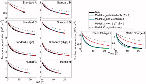
Figure 15. Particle surface area concentration throughout the duration of experiments. The same conclusions as in Figure 14 are drawn here. For all the cases, the optimized models match the data well. Again, for experiments “A”–“H,” the final selected parameters lead to a surface-area-concentration evolution that matches the data but for experiments “I” and “J,” the static charge experiments. Since surface area concentration is used for calculating the rate of vapor uptake in SOA formation experiments, fits of the surface area concentrations using the final selected values of k_e and are highly relevant.

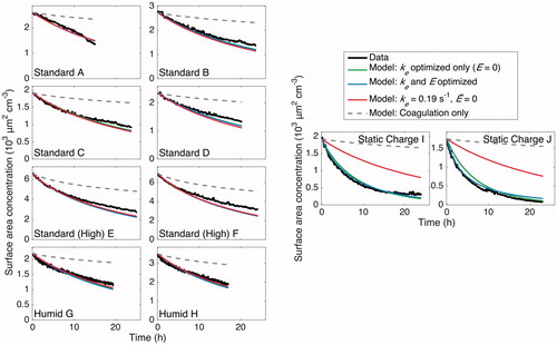
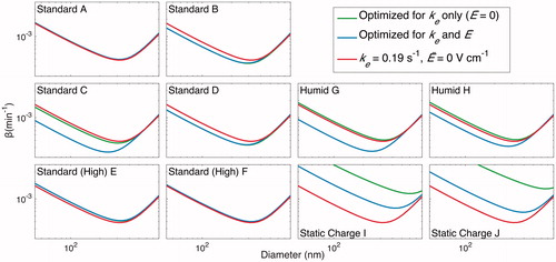
Figure 16. Resulting wall-deposition curves for the final selected parameters (k_e = 0.19 s^–1 and ) are compared to that determined by minimizing J for each experiment when only k_e is allowed to vary ( set to 0) and when both k_e and are subject to optimization. The former represents an uncharged chamber in which the electric field has no effect on the wall deposition. Note that, rigorously speaking, all curves are , the wall-deposition parameter for neutrally charged particles. Except for the static charge experiments, in which one would expect the charges on particles to be influential, the wall-deposition curve obtained is similar to both the curve found from assuming there is zero charge and from that found assuming charge is present. As in Figures 14 and 15, the final selected wall-deposition curve fits well for all but the static charge cases.

Since it has been established that one can assume  = 0, we performed a one-parameter optimization of all the “Standard” experiments together and obtained k_e = 0.19 s^–1. This optimal set of parameters fits the data well (shown in red in Figures 14 and 15) for all except the “Static Charge” experiments, in which the substantial charge on the chamber walls precludes such a fit. These parameters also fit well to the wall-deposition curves optimized for each individual experiment, shown in red in Figure 16 (again, all except for the “Static Charge” experiments, as expected).

In application to SOA experiments, the fit to the total surface area concentration (Figure 15) is especially important because, since the transport of vapor molecules to particles depends on particle surface area, SOA yield depends on the aerosol surface area concentration.

7. Conclusion

Despite the early recognition that aerosol dynamic experiments carried out in Teflon chambers may be subject to particle charging effects, no comprehensive evaluation of the role of particle charge in such experiments has previously been available. Here, using observed chamber dynamics and computational simulations, we show that the dynamics of particle-particle coagulation are essentially unaffected by particle charge under typical chamber operating conditions as long as the positive and negative ions in the surrounding area are of about equal concentration, as is the case when characteristic urban indoor ion concentrations are taken.

The ratio of positively charged particles taken directly from the chamber to those that reached the Wiedensohler distribution after leaving the chamber is constant for a typical experiment (Figure 9), the number-concentration evolution for the humid experiments does not differ significantly from that of the standard experiments (Figure 10), a two-parameter optimization procedure gives  = 0 for most of the “Standard” experiments (Figure 11), and the assumption of an average electric field of 0 gives good fits for both humid and standard operating condition experiments (Figure 14). We are able to conclude, therefore, that the standard experiments are subject to a negligible electric field, and that any electric field present is insignificant for the analysis of particle wall deposition. Furthermore, since the wall-deposition curves , as individually optimized, do not vary noticeably from those based on the optimal k_e value of 0.19 s^–1 (Figure 16), one can use the wall-deposition curve produced by assuming k_e = 0.19 s^–1 and  = 0 for all experiments performed under standard operating conditions in the Caltech Environmental Chamber.

Ideally, there would be no static charge on the walls of environmental chambers. This would allow the use of a constant from experiment to experiment and, by preventing any charge preference for particles within the chamber, minimally affect the rate of coagulation. Unfortunately, charge is too easily induced on Teflon walls: simply brushing one’s clothes or hair against a chamber is enough to induce a measurable static charge. We provide here three methods for discerning the state of a static charge on Teflon chamber walls that can be applied to other chambers.

Acknowledgments

We thank Jeffrey R. Pierce for helpful suggestions.

Additional information

Funding

SMC acknowledges support by a National Science Foundation Graduate Research Fellowship under [Grant No. 1745301]. This work was also supported by National Science Foundation [grants AGS-1523500 and AGS-1740552].

References

- Chen, J., and Wang, Z. L. (2017). Reviving Vibration Energy Harvesting and Self-Powered Sensing by a Triboelectric Nanogenerator. Joule, 1:480–521.
- Crump, J. G., and Seinfeld, J. H. (1981). Turbulent Deposition and Gravitational Sedimentation of an Aerosol in a Vessel of Arbitrary Shape. J. Aerosol Sci., 12:405–415.
- Funer, R. E., and James, D. B. (1993). New Thermoplastics and Their Properties, in Polymers for Electronic and Photonic Applications, chapter Advances in Thermoplastics for Electronic Applications, C. Wong, ed., Academic Press, Inc, San Diego, pp. 339–362.
- Ghosh, K., Tripathi, S., Joshi, M., Mayya, Y., Khan, A., and Sapra, B. (2017). Modeling Studies on Coagulation of Charged Particles and Comparison with Experiments. J. Aerosol Sci., 105:35–47.
- Harrison, R., and Aplin, K. (2007). Water Vapour Changes and Atmospheric Cluster Ions. Atmos. Res., 85:199–208.
- Hirsikko, A., Nieminen, T., Gagné, S., Lehtipalo, K., Manninen, H. E., Ehn, M., Hõrrak, U., Kerminen, V.-M., Laakso, L., McMurry, P. H., Mirme, A., Mirme, S., Petäjä, T., Tammet, H., Vakkari, V., Vana, M., and Kulmala, M. (2011). Atmospheric Ions and Nucleation: A Review of Observations. Atmos. Chem. Phys., 11:767–798.
- Hirsikko, A., Yli-Juuti, T., Nieminen, T., Vartiainen, E., Laakso, L., Hussein, T., and Kulmala, M. (2007). Indoor and Outdoor Air Ions and Aerosol Particles in the Urban Atmosphere of Helsinki: characteristics, Sources and Formation. Boreal Environ. Res., 12:295–310.
- Lagarias, J. C., Reeds, J. A., Wright, M. H., and Wright, P. E. (1998). Convergence Properties of the Nelder-Mead Simplex Method in Low Dimensions. SIAM J. Optim., 9:112–147.
- McMurry, P. H., and Rader, D. J. (1985). Aerosol Wall Losses in Electrically Charged Chambers. Aerosol Sci. Technol., 4:249–268.
- Nah, T., McVay, R. C., Pierce, J. R., Seinfeld, J. H., and Ng, N. L. (2017). Constraining Uncertainties in Particle-Wall Deposition Correction during Soa Formation in Chamber Experiments. Atmos. Chem. Phys., 17:2297–2310.
- Pierce, J. R., Engelhart, G. J., Hildebrandt, L., Weitkamp, E. A., Pathak, R. K., Donahue, N. M., Robinson, A. L., Adams, P. J., and Pandis, S. N. (2008). Constraining Particle Evolution from Wall Losses, Coagulation, and Condensation-Evaporation in Smog-Chamber Experiments: Optimal Estimation Based on Size Distribution Measurements. Aerosol Sci. Technol., 42:1001–1015.
- Reiter, R. (1985). Part B: Frequency Distribution of Positive and Negative Small Ion Concentrations, Based on Many Years’ Recordings at Two Mountain Stations Located at 740 and 1780 m Asl. Int. J. Biometeorol., 29:223–231.
- Ribeiro, P., Raposo, M., Marat-Mendes, J., and Giacometti, J. (1992). Constant-Current Corona Charging of Biaxially Stretched Pvdf Films in Humidity-Controlled Atmospheres. IEEE Trans. Elect. Insul., 27:744–750.
- Seinfeld, J. H., and Pandis, S. N. (2016). Atmospheric Chemistry and Physics: From Air Pollution to Climate Change. John Wiley & Sons, Hoboken, 3rd edition.
- Sessler, G. M., Alquié, C., and Lewiner, J. (1992). Charge Distribution in Teflon Fep (Fluoroethylenepropylene) Negatively Coronacharged to High Potentials. J. Appl. Phys., 71:2280–2284.
- Stolzenburg, M. R. (1988). An Ultrafine Aerosol Size Distribution Measuring System. PhD thesis, University of Minnesota.
- Sunol, A. M., Charan, S. M., and Seinfeld, J. H. (2018). Computational Simulation of the Dynamics of Secondary Organic Aerosol Formation in an Environmental Chamber. Aerosol Sci. Technol., 52:470–482.
- Tian, J., Brem, B. T., West, M., Bond, T. C., Rood, M. J., and Riemer, N. (2017). Simulating Aerosol Chamber Experiments with the Particle-Resolved Aerosol Model Partmc. Aerosol Sci. Technol., 51:856–867.
- TSI. (2013). Advanced Aerosol Neutralizer Model 3088: Operation and Service Manual. TSI Incorporated, Shoreview.
- Vartiainen, E., Kulmala, M., Ehn, M., Hirsikko, A., Junninen, H., Petäjä, T., Sogacheva, L., Kuokka, S., Hillamo, R., Skorokhod, A., Belikov, I., Elansky, N., and Kerminen, V.-M. (2007). Ion and Particle Number Concentrations and Size Distributions along the Trans-Siberian Railroad. Boreal Environment Research, 12:375–396.
- Vetelino, K. A., Story, P. R., Mileham, R. D., Feger, C., and Galipeau, D. (1997). “A Novel Surface Acoustic Wave Microsensor Technique for Polymer Surface Characterization,” In Polymer Surfaces and Interfaces: Characterization, Modification and Application, chapter Part 1. Polymer Surface Modification and Characterization, K. L. Mittal, and K.-W. Lee, eds., VSP BV, Utrecht, pp. 101–108.
- Wiedensohler, A. (1988). An Approximation of the Bipolar Charge Distribution for Particles in the Submicron Size Range. J. Aerosol Sci., 19:387–389.